Abstract
Purpose
Model based iterative reconstruction (MBIR) algorithms such as penalized-likelihood (PL) methods have data-dependent and shift-variant image properties. Predictors of local reconstructed noise and resolution have found application in a number of methods that seek to understand, control, and optimize CT data acquisition and reconstruction parameters in a prospective fashion (as opposed to studies based on exhaustive evaluation). However, previous MBIR prediction methods have relied on idealized system models. In this work, we develop and validate new predictors using accurate physical models specific to flat-panel CT systems.
Methods
Novel predictors for estimation of local spatial resolution and noise properties are developed for PL reconstruction that include a physical model for blur and correlated noise in flat-panel cone-beam CT (CBCT) acquisitions. Prospective predictions (e.g., without reconstruction) of local point spread function and and local noise power spectrum (NPS) model are applied, compared, and validated using a flat-panel CBCT test bench.
Results
Comparisons between prediction and physical measurements show excellent agreement for both spatial resolution and noise properties. In comparison, traditional prediction methods (that ignore blur/correlation found in flat-panel data) fail to capture important data characteristics and show significant mismatch.
Conclusion
Novel image property predictors permit prospective assessment of flat-panel CBCT using MBIR. Such predictors enable standard and task-based performance assessments, and are well-suited to evaluation, control, and optimization of the CT imaging chain (e.g., x-ray technique, reconstruction parameters, novel data acquisition methods, etc.) for improved imaging performance and/or dose utilization.
Keywords: Local point spread function, noise power spectrum, CT image quality, image assessment
1. INTRODUCTION
Recently, CT image quality assessment has been a topic of increasing discussion. Two major elements of this discussion are: 1) that modern MBIR has complex image properties with shift-variant spatial resolution properties and nonstationary noise characteristics that are substantially different than traditional reconstruction approaches; and 2) that conventional image quality metrics (e.g, contrast-to-noise ratio) fail to capture important aspects of imaging performance. As such, assessment is trending toward local measures that capture location- and data-dependent image properties, and more complete local characterizations of resolution and noise that may be used as inputs to task-based metrics like detectability index to quantify task performance. Such task-based descriptors have been used for optimization of system design,1 reconstruction parameters,2 and acquisition methods.3
Analysis of resolution4 and noise5 properties for a specific class of MBIR – quadratically penalized-likelihood (PL) reconstruction – was previously investigated and found to be well-described by local point spread functions (PSFs) and local covariance. However, those analyses presumed an idealized CT system model without detector blur or noise correlations. Previous work in emission tomography6 reported that such assumptions are not valid for physical imaging system with blur, as well for flat-panel cone-beam CT (CBCT). In this work, we follow the general approach of prior work but expand system models to include flat-panel-specific effects, to develop predictive models of local noise and resolution for flat-panel CBCT using PL reconstruction. We calibrate these models in CBCT test-bench experiments and validate the predictors in physical phantom experiments.
2. THEORETICAL AND EXPERIMENTAL METHODS
2.1 Prediction of Local Resolution Properties
This work focuses on PL reconstruction with a quadratic penalty. This estimator can be written implicitly as the maximizer of the following objective function,
| (1) |
| (2) |
where represents the image volume as a vector of attenuation coefficients, is the vector of CT scanner measurements, and μ̂ denotes the reconstructed image. The objective function includes a Poisson likelihood term L and a quadratic roughness penalty term βR where β controls the overall resolution-noise tradeoff. The term ȳ represents the model of the mean measurements (i.e., the forward model).
PL reconstructed images have shift-variant resolution properties dependent on acquisition parameters, system geometry, and patient anatomy. Previous investigations4 have found that resolution properties are locally linear and shift-invariant for quadratic PL. As such we may explore the local PSF at jth voxel as
| (3) |
| (4) |
where ej specifies an image location as indicated by a unit vector with 1 for the jth element and zeros otherwise. Here, Ȳrecon is the idealized forward model adopted in reconstruction, and Ȳacq is the actual acquisition forward model that includes physical effects like detector blur. For example, one may write
| (5) |
| (6) |
where the reconstruction model presumes ideal, unblurred projections (denoted by ideal projector matrix A) while the actual flat-panel acquisition model exhibits blur (denoted by B). Following previous mathematical derivations,5 a local PSF may be derived
| (7) |
where R is the Hessian of the penalty and W is a statistical weighting matrix which is data-dependent and approximated as D{Yacq}. That is, the local PSF (and below, local noise properties) requires only a projection data estimate (e.g., the measurements), and reconstruction of the data is not required. This expression captures the location-dependence (j), the data-dependence (W), and dependence on reconstruction parameters and regularization (βR). The idealized resolution predictor4 presumes Ȳacq = Ȳrecon and B does not appear in (7).
2.2 Prediction of Local Noise Properties
Again following previous work,5 the local covariance of μ̂ can be expressed as the jth column of
| (8) |
Traditionally, CT measurements are presumed independent making Cov{Yacq} the diagonal matrix D{Ȳacq}. A more realistic model7 for flat-panel detectors with a scintillator and stochastic blurring may be expressed as
| (9) |
where S denotes the noise power spectrum (NPS) of input/output signals, σ2 represents the variance and T denotes the MTF of detector. The parameters k and b control the relative strengths of noise that is correlated by the detector MTF and the noise that is uncorrelated, respectively.
Combining (8) and (9), the flat-panel-specific predictor of local covariance in PL CBCT is
| (10) |
where au and av are the detector pixel size. By contrast, the idealized noise predictor is
| (11) |
Since predictors in 7 and 10 include computationally expensive matrix inverses, local Fourier approximations 8 are applied to estimate the local PSF and local NPS (Fourier transform of the local covariance):
| (12) |
| (13) |
here ℱ{·} denotes discrete 3D Fourier transform and ℱ−1{·} denotes the inverse transform. Once the projection measurements (W), system geometry (A) and impulse location j are known, the local resolution and noise properties with arbitrary reconstruction parameter β are predicted with a forward and backward projection computation. By contrast, the idealized resolution and noise predictors are,
| (14) |
| (15) |
2.3 System Blur and Noise Model Validation and Measurement
To validate the resolution or noise predictors with a realistic models, we measured and modeled system blur and NPS in a flat-panel cone-beam CT (CBCT) system. As in previous work,9 we used a 5 mm thick tungsten plate to estimate a blur kernel via an edge response.10 Detector blur was estimated using five different orientations (10°, 15°, 20°, 70° and 75°) of the tungsten edge to obtain 1D detector MTFs. These experiments were repeated with the tungsten edge at the center of rotation to estimate the total system blur (including focal spot blur).
For the detector noise model, parameters k and b in (9) need to be estimated. To validate the model and find the parameter estimates, we first measured detector NPS under various exposures.11 Under an isotropic assumption, each 2D NPS is radially averaged to compute a 1D NPS profile. After normalization by variance, we fit the measured NPS profile to the model in (9), where the MTF-squared profile is obtained from the above measurements. This fitting procedure yields parameter estimates for k and b.
2.4 Resolution and Noise Properties Prediction and Measurement in CBCT Bench Data
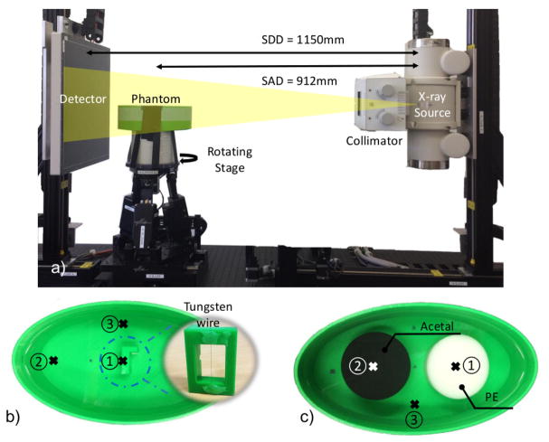
We seek validation of both resolution and noise predictors with physical experiments using the CBCT test-bench (Figure 1a). A water-filled elliptical phantom was used for each investigation. For the resolution investigation, a tungsten wire (ϕ=127 μm) was placed in three different locations to measure local 2D PSFs (Figure 1b). The wire is thin and high-contrast, making it a good physical approximation to an ideal impulse. To estimate the PSF, a water value was calculated from an annulus surrounding the wire and subtracted from the volume. Gaussian fitting was used to find the wire center over 20 axial slices. Subpixel centering was used to estimate the response on a finer grid. After deconvolving the in-plane spread function with wire cross section model and normalization, we obtain a 2D PSF that corresponds to a integral of the 3D PSF over the axial direction.
Figure 1.
Details of the physical experiments including: a) The CBCT test bench setup. b) The resolution phantom with a tungsten wire. The wire was fixed in three different positions to explore shift-variant resolution properties. c) The noise phantom with two uniform cylindrical inserts. Three positions are chosen for noise properties validation.
For the noise investigation, two uniform cylinders (one polyethylene and one acetal) were inserted in the phantom (Figure 1c). Two repeated scans were acquired, reconstructed, and subtracted to form a noise-only image volume. Presuming local stationarity, a 3D NPS was estimated using a sliding window technique with 9 3D ROIs (regions-of-interest, placed axially and half-overlapped in the z-direction).
Quadratic PL was applied with a first-order neighborhood and pairwise voxel differences, and 0.3 mm cubic voxels for noise studies and 0.2 mm for resolution studies. All local computations used a cubic ROI 71 voxels on a side. Barebeam fluence for projection data was estimated, through variance calculations with no object in the scanner, as 4.3 × 10⁴ and 6.0 × 10⁴ photons/pixel for resolution and noise studies, respectively. A separable quadratic surrogates algorithm12 used a separable footprints projector13 and 600 iterations to find the PL reconstruction. Regularization strength (β) was 105 for resolution and 106 for noise studies, respectively.
3. RESULTS
3.1 System Characteristics Measurement
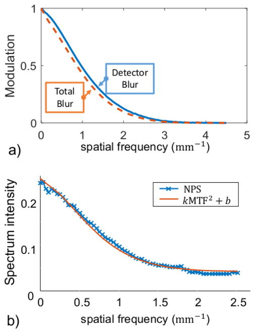
Results from the CBCT bench characterization of resolution are summarized in Figure 2a. Since little variation was found as a function of angle, only the average 1D MTF is shown in Figure 2a. The detector PSF is ~1.04 mm FWHM. Total system blur (measured at the center-of-rotation) is only slightly larger than the detector blur. This is consistent with nominal x-ray tube specifications of a 0.4 mm focal spot size. Based on a system magnification of 1.26, this focal spot will introduce less than 0.1 mm blur.
Figure 2.
a) Detector blur and system blur measured with a tungsten edge. b) Measured projection NPS and fitted, modeled NPS based on the measured detector MTF.
With the measured detector MTF and NPS measurements for different exposures, we performed a linear regression to fit the squared MTF to the angularly averaged NPS profile. The measurements and fitted model are shown in Figure 2b. We estimate model parameters k = 0.2123, b = 0.0441, which demonstrate a relatively good fit to the measurements with RMSE lower than 0.1%.
3.2 Validation of the Spatial Resolution Predictor
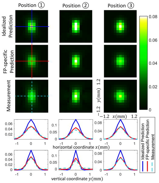
Figure 3 shows predicted and measured local PSF images. The local 2D PSF, the integral of the local 3D PSF along axial direction that corresponds to a infinitely thin line response, is shown for three different locations. The idealized local PSF predictions without a blurring kernel, new flat-panel-specific (FP-specific) PSF predictions, and wire-based PSF measurements are shown in each row. Both the shift-variant and anisotropic spatial resolution properties are evident across the three positions with greater anisotropy in positions 1 and 2 than in position 3. This is reflected in both the idealized and new FP-specific predictions. The FP-specific predictions are a better match to the measurement data. This is most evident in horizontal and vertical profiles through the PSF slices (shown at the bottom of Figure 3). Intuitively, the mismatch in the idealized predictors showed decreased blur as compared with the measurements since the blur due to the flat panel and x-ray source has not been integrated into the predictive model.
Figure 3.
Predicted versus measured local PSFs.
The greatest mismatch between the measured PSF and the predicted PSF for the new FP-specific predictor occurs at location 2. This may result from the incomplete modeling of the shift-variant focal spot blur. Since the system blur was approximated with edge measurements from the center of rotation, there may be increasing mismatches due to changes in the apparent focal spot size for more oblique measurements. To achieve a more accurate prediction, one could build a complete focal spot blur model and apply a shift-variant blurring kernel.
3.3 Validation of the Noise Predictor
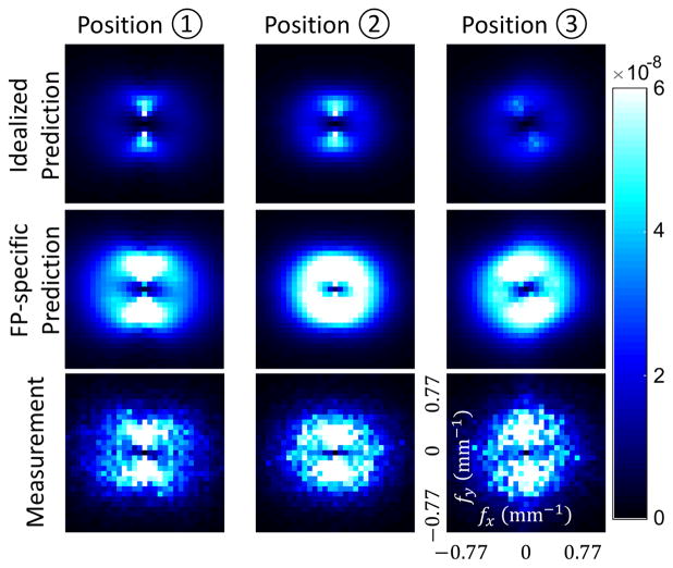
Each column of Figure 4 shows predicted and measured local NPS at three locations illustrating noise nonstationary. A central slice of the 3D NPS (fz = 0) is shown for each predictor and from phantom measurements in each row. Despite the noise in the measured NPS, the magnitude and shape of measured NPS are matched well with the predictions of the FP-specific NPS predictor. By contrast, the traditional idealized prediction model underestimates noise level by 70% and the shape of the NPS is inconsistent with measurements.
Figure 4.
Predicted versus measured local NPS.
4. DISCUSSION AND CONCLUSION
New prospective resolution and noise predictors for flat-panel CBCT were presented. To our knowledge, this is the first time such predictors have been developed and validated in physical experiments. The results show that our new predictors can precisely capture local resolution and noise properties in CBCT data, whereas idealized predictors have substantial mismatches. Since these estimates integrate the dependence on the specific acquisition, reconstruction parameters, and patient anatomy; these tools are suitable for prospective design of desirable image properties and system performance either directly through specification of noise and resolution properties or through more sophisticated task-based metrics that use the local PSF and local NPS as inputs to an observer model.
Acknowledgments
This work was supported in part by the NIH grant U01EB018758.
References
- 1.Xu J, Sisniega A, Zbijewski W, Dang H, Stayman JW, Wang X, Foos DH, Aygun N, Koliatsos VE, Siewerdsen JH. Modeling and design of a cone-beam CT head scanner using task-based imaging performance optimization. Physics in Medicine and Biology. 2016;61(8):3180–3207. doi: 10.1088/0031-9155/61/8/3180. [DOI] [PubMed] [Google Scholar]
- 2.Dang H, Stayman JW, Xu J, Sisniega A, Zbijewski W, Wang X, Foos DH, Aygun N, Koliatsos VE, Siewerdsen JH. Task-based regularization design for detection of intracranial hemorrhage in cone-beam CT. The Fourth International Conference on Image Formation in X-ray Computed Tomography; 2016. pp. 557–560. [PMC free article] [PubMed] [Google Scholar]
- 3.Gang GJ, Siewerdsen JH, Stayman JW. Task-Driven Tube Current Modulation and Regularization Design in Computed Tomography with Penalized-Likelihood Reconstruction. Physics in medicine and biology. 2016 doi: 10.1117/12.2216387. [DOI] [PMC free article] [PubMed] [Google Scholar]
- 4.Fessler JA, Rogers WL. Spatial resolution properties of penalized-likelihood image reconstruction: Space-invariant tomographs. IEEE Transactions on Image Processing. 1996;5(9):1346–1358. doi: 10.1109/83.535846. [DOI] [PubMed] [Google Scholar]
- 5.Fessler JA. Mean and variance of implicitly defined biased estimators (Such as penalized maximum likelihood): Applications to tomography. IEEE Transactions on Image Processing. 1996;5(3):493–506. doi: 10.1109/83.491322. [DOI] [PubMed] [Google Scholar]
- 6.Fessler JA. tech rep. University of Michigan; Ann Arbor: Mar, 1997. Spatial Resolution Properties of Penalized Weighted Least-Squares Tomographic Image Reconstruction with Model Mismatch. [Google Scholar]
- 7.Rabbani M, Shaw R, Van Metter R. Detective quantum efficiency of imaging systems with amplifying and scattering mechanisms. Journal of the Optical Society of America A, Optics and image science. 1987;4(5):895–901. doi: 10.1364/josaa.4.000895. [DOI] [PubMed] [Google Scholar]
- 8.Stayman J Webster, Fessler JA. Regularization for uniform spatial resolution properties in penalized-likelihood image reconstruction. IEEE Transactions on Medical Imaging. 2000;19(6):601–615. doi: 10.1109/42.870666. [DOI] [PubMed] [Google Scholar]
- 9.Wang W, Gang GJ, Stayman JW. Spatial Resolution Properties in Penalized-Likelihood Reconstruction of Blurred Tomographic Data. International Conference on Fully Three-Dimensional Image Reconstruction in Radiology and Nuclear Medicine; Xi’an, China. 2017. [Google Scholar]
- 10.Samei E, Flynn MJ, Reimann DA. A method for measuring the presampled MTF of digital radiographic systems using an edge test device. Medical physics. 1998;25(1):102–113. doi: 10.1118/1.598165. [DOI] [PubMed] [Google Scholar]
- 11.Siewerdsen JH, Antonuk LE, El-Mohri Y, Yorkston J, Huang W, Cunningham IA. Signal, noise power spectrum, and detective quantum efficiency of indirect-detection flat-panel imagers for diagnostic radiology. Medical Physics. 1998;25(5):614–628. doi: 10.1118/1.598243. [DOI] [PubMed] [Google Scholar]
- 12.Erdogan H, Fessler JA. Ordered subsets algorithms for transmission tomography. Physics in medicine and biology. 1999;44(11) doi: 10.1088/0031-9155/44/11/311. [DOI] [PubMed] [Google Scholar]
- 13.Long Y, Fessler JA, Balter JM. 3D forward and back-projection for X-ray CT using separable footprints. IEEE Transactions on Medical Imaging. 2010;29(11):1839–1850. doi: 10.1109/TMI.2010.2050898. [DOI] [PMC free article] [PubMed] [Google Scholar]


