Variable Selection in Kernel Regression Using Measurement Error Selection Likelihoods

Abstract

This paper develops a nonparametric shrinkage and selection estimator via the measurement error selection likelihood approach recently proposed by Stefanski, Wu, and White. The Measurement Error Kernel Regression Operator (MEKRO) has the same form as the Nadaraya-Watson kernel estimator, but optimizes a measurement error model selection likelihood to estimate the kernel bandwidths. Much like LASSO or COSSO solution paths, MEKRO results in solution paths depending on a tuning parameter that controls shrinkage and selection via a bound on the harmonic mean of the pseudo-measurement error standard deviations. We use small-sample-corrected AIC to select the tuning parameter. Large-sample properties of MEKRO are studied and small-sample properties are explored via Monte Carlo experiments and applications to data.

1 Introduction

Stefanski, Wu, and White (henceforth SWW; Stefanski et al., 2014) describe a very general variable selection method that results from modeling predictors as if they were contaminated with measurement error. A model is first embedded in a measurement error model (MEM) framework, then the resulting MEM selection likelihood is maximized subject to a lower bound on the total measurement error. The feasible region set by the constraints has sharp corners that admit feature sparsity. The total measurement error serves as a tuning parameter to balance model sparsity and fit.

When applied to linear models, the SWW procedure generates solution paths identical to those of LASSO (Stefanski et al., 2014; Tibshirani, 1996). Thus, one can regard SWW’s procedure as an extension of LASSO to any model—in this paper, to nonparametric regression. We show that applying the SWW procedure to nonparametric regression results in the Nadaraya-Watson (NW) estimator, but with a novel method of bandwidth estimation that simultaneously performs smoothing and finite-sample variable selection as demonstrated by our simulation studies. Though bandwidth selection is much studied for the NW estimator, variable selection is less studied and generally only asymptotically. The measurement error kernel regression operator (MEKRO) integrates both.

Intentionally contaminating observations with noise has been previously studied under the terms “noise injection” or “training with noise,” among others. Predictor contamination is well-studied in general for artificial neural networks where small amounts of noise reduce overfitting and generalization error (Sietsma and Dow, 1991; Grandvalet and Canu, 1995; Grandvalet et al., 1997; Holmstrom and Koistinen, 1992). Simulation-extrapolation (SIMEX) estimation is a method to correct for measurement error in predictors by adding increasing amounts of known measurement error and extrapolating back to a hypothetical version of the data without error (J. R. Cook, 1994; Stefanski and Cook, 1995). Importantly, our method is distinguished from these noise-addition methods; we develop a likelihood under the false assumption that noise is present instead of contaminating observations.

This paper is organized as follows. Derivation of MEKRO and computational aspects of fitting and tuning are presented in Section 2. We extend the method to accomodate categorical covariates in Section 3. Section 4 describes related methods in the literature and provides numerical support for MEKRO with both simulated and real data examples. In Section 5 we study selection consistency. Section 6 closes with a discussion.

We observe data $\{{\left({\mathit{X}}_i,Y_i\right)}_{i=1}^n\}$, where Y_i is the response, X_i = (X_i,1, …, X_i,p)^T is the p × 1 vector of covariates for the ith observation, and p is fixed. The (continuous) covariates are standardized so that ${\displaystyle {\sum }_{i=1}^n{\mathit{X}}_i={\mathbf{0}}_{p\times 1}}$ and ${\displaystyle {\sum }_{i=1}^n{X}_{i,j}^2}/(n-1)=1$, j = 1, …, p. Denote a generic observation as (X, Y) where X has jth component X_j. We assume the model

$$Y=g(\mathit{X})+\epsilon ,$$ (1)

where $g(\mathit{x})=g_{Y|\mathit{X}}(\mathit{x})\stackrel{\text{def}}{=}E(Y|\mathit{X}=\mathit{x})$ is the unknown regression function, and ε is a random error independent of X with E(ε) = 0 and $\mathrm{E}({\epsilon }^2)={\sigma }_{\epsilon }^2<\infty$. For presentation simplicity, assume that Y and X are both continuous unless otherwise stated.

2 Measurement Error Kernel Regression Operator

In a supervised learning problem, if a covariate can be contaminated with a substantial amount of error without adversely affecting prediction performance, then it is not useful for predicting Y. Measurement error model (MEM) selection likelihoods introduced by SWW implement this concept by forcing ‘false’ Gaussian measurement error into the covariates X. We first build a selection likelihood that describes the prediction degradation for a certain allocation of measurement error to each covariate. Then we perform constrained optimization of the likelihood where the constraints force ‘false’ measurement error into the likelihood while the optimizer determines the distribution of errors that results in the least degradation. The likelihood optimization ensures that the least relevant covariates will be assigned the most (possibly infinite) error.

Denote the measurement error variance associated with X_j as ${\sigma }_{u,j}^2$. MEM selection likelihoods describe model degradation through λ_j = 1/σ_{u, j} and apply the optimization constraint 1^Tλ = τ where τ > 0 is a tuning parameter. This constraint is equivalent to an equality constraint on the harmonic mean of σ_u and allows one or more σ_{u, j} = ∞ when τ > 0, implying that each corresponding X_j can be measured with an infinite amount of ‘false’ measurement error and thus is irrelevant in the model. A constraint on the un-transformed σ_u could not achieve this as elegantly.

Applying the MEM selection likelihood framework from SWW to nonparametric regression results in a kernel regression bandwidth and variable selection method, the measurement error kernel regression operator (MEKRO). The MEM selection likelihood is

$${\widehat{L}}_{\mathrm{SEL}}(\mathit{\lambda })=-\frac{1}{n}{\displaystyle \sum _{i=1}^n{\{Y_i-\widehat{g}({\mathit{X}}_i,\mathit{\lambda })\}}^2},$$ (2)

where

$$\widehat{g}({\mathit{X}}_i,\mathit{\lambda })=\frac{{\displaystyle {\sum }_{k=1}^n{Y}_k{\displaystyle {\prod }_{j=1}^p\exp \{-{\lambda }_j^2{(X_{i,j}-X_{k,j})}^2/2\}}}}{{\displaystyle {\sum }_{k=1}^n{\displaystyle {\prod }_{j=1}^p\exp \{-{\lambda }_j^2{(X_{i,j}-X_{k,j})}^2/2\}}}}.$$ (3)

See online Appendix A for the full derivation. Notice that (2) is simply the (negative) mean squared error, and, more interestingly, (3) is the familiar Nadaraya-Watson estimator (Nadaraya, 1964; Watson, 1964) of g(⋅) from the data $\{{({\mathit{X}}_i,Y_i)}_{i=1}^n\}$, computed using a Gaussian product kernel and diagonal bandwidth matrix. One key difference is that the traditional smoothing bandwidths, h_j, are parameterized as inverse bandwidths, λ_j = 1/h_j. In this setting, λ_j = 0 ⇒ h_j = ∞, or covariate X_j is infinitely smoothed and thus selected out. This parameterization is also found in Goutte and Larsen (2000).

Estimation of the (inverse-) bandwidths is done as prescribed in SWW, via maximizing ${\widehat{L}}_{\mathrm{SEL}}(\mathit{\lambda })$ subject to an L₁-type constraint in the non-negative orthant,

$${\lambda }_j\ge 0,j=1,\dots ,p;{\displaystyle \sum _{j=1}^p{\lambda }_j=\tau ,\text{for fixed}\tau >0},$$ (4)

where τ is a tuning parameter controlling the roughness of $\widehat{g}(\cdot )$. A small τ keeps ‖λ‖ small, implying large bandwidths and substantial smoothing; a large τ permits smaller individual bandwidths and more roughness in $\widehat{g}(\cdot )$. Adding generated noise to predictors with this constraint has been successful in artificial neural networks (Grandvalet and Canu, 1997).

Although MEKRO is the focus of this paper, the derivation of an estimator using MEM selection likelihoods itself is interesting and worth highlighting. SWW proved that applying MEM selection likelihoods to the linear model is equivalent to LASSO. The proof hinged on equivalent ways to express linear model coefficients subjected to shrinkage, either through ridge regression, LASSO, or MEM selection likelihoods. Although the same relationships or concepts do not exist in more complicated models, MEM selection likelihoods have been shown via simulation to produce LASSO-like, finite-sample variable selection in a density-based classification procedure (Stefanski et al., 2014) and in kernel regression (MEKRO).

A MEKRO solution ${\widehat{\mathit{\lambda }}}_{\tau }$ is the result of optimizing ${\widehat{L}}_{\mathrm{SEL}}(\mathit{\lambda })$ under the constraints in (4). To avoid constrained optimization, we introduce γ ∈ ℝ^p and let ${\lambda }_j({\gamma }_j)=\tau {\gamma }_j^2/\left({\displaystyle {\sum }_{k=1}^p{\gamma }_k^2}\right)$, j = 1, …, p, for a fixed τ. We then maximize ${\widehat{L}}_{\mathrm{SEL}}(\mathit{\lambda }(\mathit{\gamma }))$ with respect to γ. This guarantees that the constraints (4) on λ are satisfied for any γ, at the cost of one additional parameter. Optimization is done in C using the gradient-based algorithm L-BFGS (Okazaki, 2010). With ${\pi }_{ik}={\displaystyle {\prod }_{j=1}^p\exp \{-{\lambda }_j^2{(X_{i,j}-X_{k,j})}^2/2\}}$ and $\mathrm{\Gamma }={\displaystyle {\sum }_{j=1}^p{\gamma }^2}$, then $\widehat{g}({\mathit{X}}_i,\mathit{\lambda })={\displaystyle {\sum }_{k=1}^n{Y}_k{\pi }_{ik}}/{\displaystyle {\sum }_{k=1}^n{\pi }_{ik}}$ and the required gradients are,

$$\begin{array}{l}\partial \widehat{g}({\mathit{X}}_i,\mathit{\lambda })/\partial {\lambda }_t=[{\displaystyle \sum _{k=1}^n{Y}_k{\pi }_{ik}\{-{\lambda }_t{\left(X_{i,t}-X_{k,t}\right)}^2\}}\times {\displaystyle \sum _{k=1}^n{\pi }_{ik}-}\\ {\displaystyle \sum _{k=1}^n{\pi }_{ik}\{-{\lambda }_t{\left(X_{i,t}-X_{k,t}\right)}^2\}}\times {\displaystyle \sum _{k=1}^n{Y}_k{\pi }_{ik}}]{\left({\displaystyle \sum _{k=1}^n{\pi }_{ik}}\right)}^{-2}.\end{array}$$

Also, $\partial {\lambda }_t/\partial {\gamma }_j=-2\tau {\gamma }_t^2{\gamma }_j{\mathrm{\Gamma }}^{-2}$ when t ≠ j and $2\tau {\gamma }_j(\mathrm{\Gamma }-{\gamma }_t^2){\mathrm{\Gamma }}^{-2}$ when t = j. Finally,

$$\partial {\widehat{L}}_{\mathrm{SEL}}/\partial {\gamma }_j=\frac{4\tau {\gamma }_j}{n{\mathrm{\Gamma }}^2}{\displaystyle \sum _{t=1}^p\left[{\displaystyle \sum _{i=1}^n\{Y_i-\widehat{g}({\mathit{X}}_i,\mathit{\lambda })\}\times }(\partial \widehat{g}({\mathit{X}}_i,\mathit{\lambda })/\partial {\lambda }_t)\right]}({\gamma }_t^2-\mathrm{\Gamma }{\mathrm{𝟙}}_{t=j}),$$ (5)

where 𝟙_(⋅) is the indicator function. ${\widehat{L}}_{\mathrm{SEL}}(\mathit{\lambda })$ is not concave but can be maximized well with neutral starting values. However, starting values near where at least one component of λ is zero and the initial gradient points in an unfavorable direction tends to trap the optimizer in non-global maxima. Further, (5) shows that $\partial {\widehat{L}}_{\mathrm{SEL}}/\partial {\gamma }_j$ is 0 when γ_j = 0. Thus, using warm starts with components of λ set at or near 0 is ill-advised. We always start at γ_start = 1_p, equivalent to λ_start = (τ/p)1_p.

2.1 Example

We generate n = 100 iid observations from the model,

$$Y=\sin (2\pi X_1)+\sin (\pi X_2)+0.5\epsilon ,$$ (6)

where p = 3, X₁, X₂, X₃ ~ U(0, 1) and ε ~ N(0, 1), independent of X. The X₁ component has the same amplitude but oscillates twice as quickly as the X₂ component, and thus X₁ is more important in describing the variation in Y; X₃ is an irrelevant predictor.

Figure 1 illustrates how the inverse-bandwidth parameterization and constraint (4) encourages sparse solutions.

Figure 1.

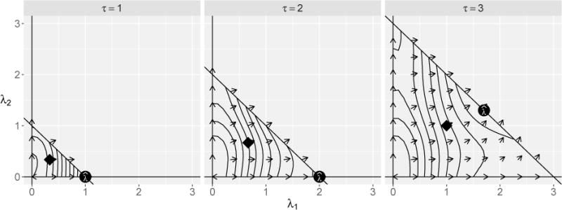
${\widehat{L}}_{\mathrm{SEL}}(\mathit{\lambda })$contours and gradient vector fields of example model (6) for λ = (λ₁, λ₂, λ₃ = τ − λ₁ − λ₂) and τ ∈ {1, 2, 3}; global maxima are denoted with solid circles and the neutral starting values λ_start = (τ/p)1_p are denoted with solid diamonds.

When τ = 1, the smallest kernel bandwidth, h, permitted in g(⋅) is h = 1/τ = 1, which results in considerable smoothing (recall that each X_j is scaled to have mean zero and unit variance before fitting, so at τ = 1 the data and kernel weights have equal variances). When such a smooth model is forced, the maximizer of ${\widehat{L}}_{\mathrm{SEL}}(\mathit{\lambda })$ rests in a corner of the feasible region defined by the constraints at ${\widehat{\mathit{\lambda }}}_{\tau }=(1,0,0)$. At this solution, both λ₂ and λ₃ have infinite kernel bandwidths and X₂ and X₃ are selected out. When τ = 2, maximizing ${\widehat{L}}_{\mathrm{SEL}}(\mathit{\lambda })$ still results in the solution ${\widehat{\mathit{\lambda }}}_{\tau }=(\tau ,0,0)$, however, the contours hint at the importance of X₂ by bending along the diagonal boundary. When more roughness is permitted at τ = 3, the maximizer slides along the boundary and splits τ between λ₁ and λ₂, leaving λ₃ = 0 (note that solutions along the line λ₂ = τ − λ₁ imply that λ₃ = 0). As τ increases, the maximizer approaches (τ/3)1₃ and results in overfitting (plot not shown).

2.2 Tuning and Solution Paths

An optimal τ is chosen via small-sample nonparametric AIC, AIC_c, suggested in Hurvich et al. (1998) resulting in a sparse inverse-bandwidth solution ${\widehat{\mathit{\lambda }}}_{\tau }$. Cross-validation is prohibitively slow. In preliminary simulation studies, AIC_c worked as well or better than other criteria (Hastie et al., 2009). The degrees of freedom are approximated by tr(S_τ), where S_τ is the n × n smoothing matrix with [r, s] element,

$${\mathit{S}}_{\tau }[r,s]={\frac{{\displaystyle {\prod }_{j=1}^p\exp \{-{\lambda }_j^2{(X_{s,j}-X_{r,j})}^2/2\}}}{{\displaystyle {\sum }_{k=1}^n{\displaystyle {\prod }_{j=1}^p\exp \{-{\lambda }_j^2{(X_{r,j}-X_{k,j})}^2/2\}}}}|}_{\mathit{\lambda }={\widehat{\mathit{\lambda }}}_{\tau }}.$$ (7)

Thus, $\widehat{\tau }$ minimizes,

$${\mathrm{AIC}}_c(\tau )=\ln \{-{\widehat{L}}_{\mathrm{SEL}}({\widehat{\mathit{\lambda }}}_{\tau })\}+\frac{n+\text{tr}({\mathit{S}}_{\tau })}{n-\text{tr}({\mathit{S}}_{\tau })-2}.$$

In practice, we first compute ${\widehat{\tau }}_0=\arg {\min }_{\tau \in \mathit{\tau }\ast }{\mathrm{AIC}}_c(\tau )$, where τ^* is a predetermined coarse grid. Then we create a finer τ^* grid around ${\widehat{\tau }}_0$ and repeat the search for the final $\widehat{\tau }$.

The plot of ${\widehat{\mathit{\lambda }}}_{\tau }$ versus τ is an inverse-bandwidth solution path, similar to LASSO solution paths. To illustrate, again consider the example from Section 2.1 except with two additional irrelevant predictors (X₄ and X₅). The solution path is shown in Figure 2; solid dots represent active predictors and open dots represent irrelevant predictors. Overlaid is the scaled AIC_c(τ) curve (dashed line). Predictor indices are shown in the right margin. In this example, $\widehat{\tau }=5$, for which ${\widehat{\lambda }}_1$, ${\widehat{\lambda }}_2>0$ and ${\widehat{\lambda }}_3={\widehat{\lambda }}_4={\widehat{\lambda }}_5=0$ (perfect selection after tuning). Note that at the final solution, the inverse-bandwidth associated with the more rapidly varying predictor (X₁) is larger than the more slowly varying one (X₂), as expected.

Figure 2.

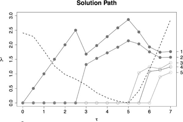
Solution paths of ${\widehat{\mathit{\lambda }}}_{\tau }$ versus τ for Section 2.1 example with two active (solid) and three irrelevant (open) predictors. Dashed line: scaled AIC_c(τ), τ ∈ τ^*= {0, 0.5, …, 7}.

3 Extension to Categorical Predictors

Let $\mathcal{C}=\{j:X_j\text{is continuous}\}$ and $\mathcal{D}=\{j:X_j\text{is categorical}\}$. If $j\in \mathcal{D}$ then assume without loss of generality that X_j takes values in the label set {0, …, D_j − 1} where there is no natural ordering. The ‘frequency approach’ (see Li and Racine, 2007) estimates a separate regression function for each permutation of observed discrete variables, but reduces the effective sample size of each separate estimator by a factor of approximately ${\displaystyle {\prod }_{j\in \mathcal{D}}{D}_j^{-1}}$. We describe an extension of MEKRO for mixed continuous and categorical variables based on the approach in Racine and Li (2004). The kernel for smoothing categorical X_j is

$$l_j(X_j,x_j)={(1-{\delta }_j)}^{{\mathrm{𝟙}}_{X_j\ne x_j}},$$ (8)

where δ_j ∈ [0, 1]. If δ_j = 0, l_j is identically equal to 1 and does not depend on X_j. If δ_j = 1, l_j is zero unless X_j = x_j. Any δ_j ∈ (0, 1) smooths the effect of covariate j, borrowing weight across the D_j different values of x_j.

Simply letting δ_j play the role of λ_j in the MEKRO algorithm fails because δ_j is bounded above by 1; thus, continuous and categorical predictors would be penalized unequally by the sum constraint in (4) because of the scaling differences. To alleviate the scaling problem, we propose the univariate categorical kernel

$$k_j^d(X_j,x_j)=\exp \left(-\frac{1}{2}{\lambda }_j^2{w}_j{\mathrm{𝟙}}_{X_j\ne x_j}\right),$$ (9)

where λ_j is the same inverse bandwidth parameter used throughout this paper, and w_j is a weight. This is similar to the continuous kernel, except that the indicator and weight replace ${\left(X_{k,j}-X_{i,j}\right)}^2$. To weight the categorical and continuous kernels similarly, note that if $j\in \mathcal{C}$, E[(X_k,j − X_i,j)²] = 2 for i ≠ k. If $j\in \mathcal{D}$, and again for i ≠ k, $\mathrm{E}[{\mathrm{𝟙}}_{X_{kj}\ne X_{ij}}]=1-P(X_{k,j}=X_{i,j})=1-{{\displaystyle {\sum }_{t=1}^{D_j}[P(X_{k,j}=t)]}}^2$. Then set $w_j=2/[1-{\displaystyle {\sum }_{t=1}^{D_j}{\{\widehat{P}(X_{k,j}=t)\}}^2}]$ where $\widehat{P}(X_{k,j}=t)=n^{-1}{\displaystyle {\sum }_{k=1}^n{\mathrm{𝟙}}_{X_{kj}=t}}$. The weight requires that realizations be spread across two or more categories. When the data are balanced across the D_j categories, the weight reduces to w_j = 2D_j/(D_j − 1). Observe that, like (8), λ_j = 0 implies that categorical covariate j is selected out, and λ_j large implies $\widehat{g}(\cdot ,\mathit{\lambda })$ is different for each category in D_j.

The estimator for g(⋅) incorporating categorical variables is then

$$\widehat{g}({\mathit{X}}_i,\mathit{\lambda })=\frac{{\displaystyle {\sum }_{k=1}^n{Y}_k{\displaystyle {\prod }_{j\in \mathcal{C}}\exp \{-{\lambda }_j^2{(X_{i,j}-X_{k,j})}^2/2\}{\displaystyle {\prod }_{j\in \mathcal{D}}\exp \left(-{\lambda }_j^2{w}_j{\mathrm{𝟙}}_{X_{kj}\ne X_{ij}}/2\right)}}}}{{\displaystyle {\sum }_{k=1}^n{\displaystyle {\prod }_{j\in \mathcal{C}}\exp \{-{\lambda }_j^2{(X_{i,j}-X_{k,j})}^2/2\}{\displaystyle {\prod }_{j\in \mathcal{D}}\exp (-{\lambda }_j^2{w}_j{\mathrm{𝟙}}_{X_{kj}\ne X_{ij}}/2)}}}},$$

where w_j is described above. This is substituted into (2) and optimized under (4) by methods in Section 2.

4 Method Comparison and Numerical Results

Much of the nonparametric regression methodology incorporating variable importance can be separated into two classes: methods that downweight features with little or no effect, and methods that perform feature subset selection. Arguments can be made for either, based on either modeling philosophy or the particular application. It is unlikely that any judicious real-world regression application includes truly irrelevant variables, and downweighting can be superior to selection for predictions when there are a larger number of small effects present (ridge regression vs. LASSO in Tibshirani, 1996). On the other hand, sparsity attained from selection is valuable for parsimonious model descriptions, avoiding the curse of dimensionality (Lafferty and Wasserman, 2008), and predictions where there are only a few large effects.

MEKRO falls into the selection class, along with several other popular methods. Friedman (1991) developed MARS, a method that flexibly estimates models using a basis of linear splines with one knot, but it is prone to overfitting (Barron and Xiao, 1991). COSSO extends smoothing spline ANOVA models to perform selection by penalizing a least-squares loss similar to that of LASSO (Tibshirani, 1996; Lin and Zhang, 2006). Adaptive COSSO uses an adjusted weighting scheme analogous to the adaptive LASSO (Storlie et al., 2011). Both versions of COSSO typically truncate the model complexity at or below two-way interactions. SPAM (sparse additive models) is similar to COSSO in that it truncates complexity, but it allows p ≫ n (Ravikumar et al., 2009). Kernel iterative feature extraction (KNIFE) by Allen (2013) imposes L₁-regularization on L₂-penalized splines.

Many of the downweighting methods are similar to MEKRO by attaching individual weights to the separate input dimensions in a flexible model. Automatic relevance determination (ARD) first described by Neal (1996) puts prior distributions on weights for each input in a Bayesian neural network, and input weights of only irrelevant predictors remain concentrated around 0. Williams and Rasmussen (1996) put weights on the distance metric for each input dimension in the covariance function of a Gaussian process and demonstrate results similar to ARD. Grandvalet and Canu (1997) add noise to each input of an artificial neural network and use the harmonic mean to control the total noise added. They show greatly reduced generalization errors against trees and k-nearest neighbors on classification problems, but do not consider examples with irrelevant inputs. Adaptive metric kernel regression (AMKR; Goutte and Larsen, 2000) is a kernel regression bandwidth selection procedure that parameterizes the local-constant estimator with inverse-bandwidths. However, it directly optimizes the leave-one-out cross-validation loss instead of MEKRO’s approach of choosing an optimal smoothness from an entire path of solutions with sparsity via cross-validation. RODEO (Lafferty and Wasserman, 2008) thresholds derivatives of the local-linear estimator to keep bandwidths associated with irrelevant variables large.

4.1 Simulation Preliminaries

This section presents numerical studies on the performance of MEKRO (MEK) against other variable selection methods for nonparametric regression, including KNIFE (KNI), two “regular” COSSO variants (additive COSSO, RC1; two-way interaction COSSO, RC2), two adaptive COSSO, or ACOSSO variants (additive ACOSSO, AC1; two-way interaction ACOSSO, AC2), and MARS (additive, M1; two-way interaction, M2; thee-way interaction, M3). We use the default GCV criterion for MARS. For KNIFE, we fix λ₁ = 1 and use a radial kernel with γ = 1/p as suggested in Allen (2013). The weight power for the ACOSSO is fixed at γ = 2, as suggested by Storlie et al. (2011). Although these parameters serve as additional tuning parameters, we tune only one parameter per method for fairness. We also include AMKR (AM) because of its close relationship with MEKRO.

Each simulation sets Y_i = g(X_i) + ε_i where ${\epsilon }_i\stackrel{\text{iid}}{\sim }\mathrm{N}(0,{\sigma }_{\epsilon }^2)$ and g(⋅) is defined for each model. We set ${\sigma }_{\epsilon }^2$ so that the theoretical model $R^2=\text{Var}\{g(\mathit{X})\}/[\text{Var}\{g(\mathit{X})\}+{\sigma }_{\epsilon }^2]$ is 0.75 (a SNR of 3) unless otherwise noted. The predictors are generated as X_j = (U_j + kU^*)/(1 + k); U_j ~ U(0, 1), j = 1, …, p; U^* ~ U(0, 1), so that X_j ∈ [0, 1] and X has compound symmetric correlation ρ = k²/(1 + k²). The covariates are independent when ρ = 0.

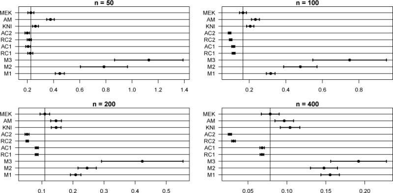
Results are summarized in terms of Type I selection error (irrelevant predictor inclusion rate), Type II selection error (active predictor exclusion rate), and average integrated squared error (AISE) over M = 100 Monte Carlo (MC) replications. AISE estimates $\mathrm{MISE}=\mathrm{E}{\{\widehat{g}(\mathit{X},{\widehat{\mathit{\lambda }}}_{\widehat{\tau }})-g(\mathit{X})\}}^2={\mathrm{E}}_T[\mathrm{E}{\{\widehat{g}(\mathit{X},{\widehat{\mathit{\lambda }}}_{\widehat{\tau }})-g(\mathit{X})\}}^2|\mathit{T}]$ by averaging the mean squared difference between $\widehat{g}(\cdot ,{\widehat{\mathit{\lambda }}}_{\widehat{\tau }})$ and g(⋅) evaluated on test data over 100 MC replicates, where T is random training data used in defining the estimator $\widehat{g}(\cdot ,{\widehat{\mathit{\lambda }}}_{\widehat{\tau }})$, and X and T follow the same distribution. We use a test set of 10,000 X data vectors for each model and vary the dimension of T as a simulation factor. AISE comparison plots (Fig. 3, 5–10) show 95% confidence bars for the MISE of each method. MISEs with non-overlapping confidence bars are statistically different based on the more powerful paired-difference test (not shown).

Figure 3.

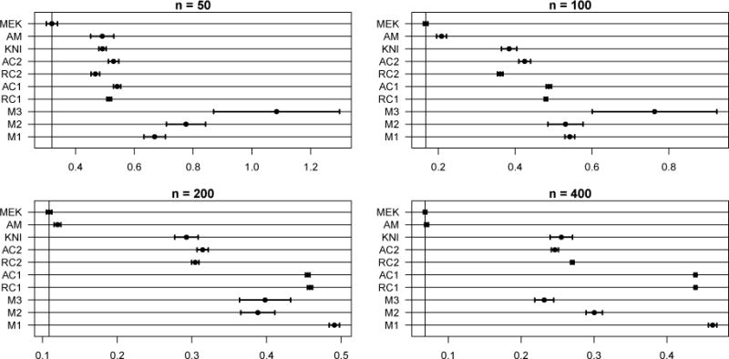
AISEs for Model 1. Note the scale differences. Out of the 400 MC samples, 3 AISE outliers are omitted from M3.

Figure 5.

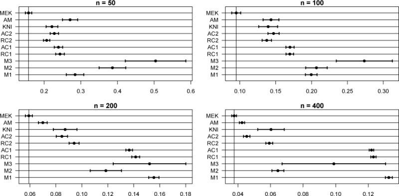
AISEs for Model 2. Note the scale differences. Out of the 400 MC samples, 19 and 6 AISE outliers are omitted from M3 and M2, respectively.

Figure 10.

AISEs (average integrated squared errors) for Appendix C Model. Note the scale differences. Out of the 400 MC samples, 2 AISE outliers are omitted from both M2 and M3.

We give a measure of predictor effect size to provide additional context to regression functions and simulation results. In models with complex interactions, it is difficult to quantify the contribution of each covariate to the regression function variance. We quantify effect size with the scaled root mean squared risk difference between the regression function with and without X_j is replaced by its mean. Define $v_j=\mathrm{E}{\{g(\mathit{X})-g(\mathit{X}{|}_{X_j=\mathrm{E}(X_j)})\}}^2$. Then the predictor effect size for X_j is defined as $v_j^{1/2}/\max \{{\mathit{v}}_j^{1/2}\}$. We compute effect sizes to two decimal places via numerical integration. When this method is applied to linear regression, the effect sizes are the scaled absolute regression coefficients. Predictors with near-zero effect sizes are effectively irrelevant and inflate Type II selection errors for all methods.

As an example, consider two models used in Friedman (1991) for assessing variable selection and prediction performance of MARS,

$$Z(X_1,X_2,X_3,X_4)={\left\{X_1^2+{(X_2{X}_3-\frac{1}{X_2{X}_4})}^2\right\}}^{1/2},\text{and}$$ (10)

$$\varphi (X_1,X_2,X_3,X_4)=\arctan \left\{\frac{X_2{X}_3-1/(X_2{X}_4)}{X_1}\right\},$$ (11)

where X₁ ∈ [0, 100], X₂ ∈ [40π, 560π], X₃ ∈ [0, 1], and X₄ ∈ [1, 11], all uniformly distributed. Both models contain all orders of interactions, although the contribution of the covariates to the model varies widely. Predictor effect sizes for active predictors (X₁, X₂, X₃, X₄) are (0.03, 0.90, 1.00, 0.00) in Z(⋅) and (0.55, 0.59, 1.00, 0.00) in ϕ(⋅). Because the contributions from X₁ in Z(⋅) and X₄ in both models are so low, Z(⋅) is well-approximated by two-way interaction models, and ϕ(⋅) is well-approximated by three-way interaction models. This was recognized in Lin and Zhang (2006) after model fitting and observing the performance of a two-way interaction model against a saturated model.

4.2 Simulation Results

Model 1

Nonlinear, three-way interaction; g(X) = sin{2π(X₁ + X₂)/(1 + X₃)}; p = 10 (7 irrelevant variables included); ρ = 0; n ∈ {50, 100, 200, 400}. Predictor effect sizes for active predictors (X₁, X₂, X₃) are (1.00, 1.00, 0.48). Selection errors are displayed in Table 1 and average integrated squared errors (AISEs) are in Figure 3. MEKRO (MEK) dominates in both prediction and selection, achieving perfect selection when n ≥ 100, and having a comparable AISE to AMKR only when n = 400. AMKR (AM) overselects irrelevant covariates. KNIFE (KNI) has approximately the same AISE as the two-way interaction COSSO models (RC2, AC2), but greatly underselects for smaller n. The two-way interaction COSSO models show a clear advantage over the additive COSSO.

Table 1.

Selection error rates for Model 1. MC standard errors for all cells ≤ 0.03.

	Error	MEK	AM	KNI	AC2	RC2	AC1	RC1	M3	M2	M1
n = 50	Type I Type II	0.05 0.13	0.55 0.06	0.09 0.73	0.14 0.58	0.19 0.49	0.29 0.53	0.19 0.62	0.56 0.21	0.54 0.21	0.70 0.19
n = 100	Type I Type II	0.00 0.00	0.46 0.00	0.05 0.40	0.24 0.36	0.11 0.42	0.27 0.40	0.12 0.46	0.49 0.04	0.52 0.05	0.64 0.12
n = 200	Type I Type II	0.00 0.00	0.48 0.00	0.03 0.17	0.26 0.31	0.08 0.38	0.31 0.22	0.07 0.36	0.28 0.00	0.38 0.00	0.65 0.12
n = 400	Type I Type II	0.00 0.00	0.52 0.00	0.03 0.10	0.22 0.31	0.05 0.39	0.30 0.20	0.04 0.31	0.07 0.00	0.22 0.00	0.65 0.09

(RC1, AC1) models for prediction in larger samples; the large effect sizes for X₁ and X₂ and smaller effect size of X₃ indicates that g(⋅) is well-approximated by a two-way interaction model but not an additive model. The three-way interaction MARS model (M3) performs worst when n ≤ 100, but demonstrates good selection rates for n = 400.

We now elaborate on the selection performance for adaptive metric kernel regression (AMKR). Simulation studies in Goutte and Larsen (2000) suggest that inverse-bandwidth estimates for irrelevant covariates are shrunk from AMKR, but are frequently positive (non-zero). Thus, for comparing to a selection method, one must select a cutoff to operationalize when an inverse-bandwidth is small enough to be selected out. Our simulation studies show that AMKR-estimated inverse-bandwidths are either near machine zero or large enough to be regarded as relevant. The left panel of Figure 4 shows the AMKR estimates for Model 1, n = 400, where X₄ through X₁₀ are irrelevant and should each have 1/h = 0. Of the 700 samples (100 MC replicates for 7 predictors), 48% of them had an AMKR estimate of 0. The right panel of Figure 4 shows the log₁₀-value for the other 52% of estimates that were positive; many clump around 10^−0.5, a smooth kernel bandwidth, but still large enough to be considered relevant. There are very few positive estimates below 10⁻⁴ even in this moderate sample size case, thus we chose a cutoff of 10⁻⁴ below which an AMKR inverse bandwidth was considered 0.

Figure 4.

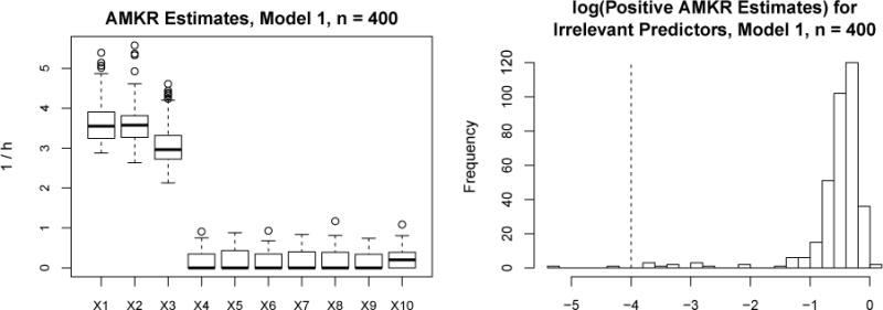
Study of AMKR estimates for Model 1, n = 400.

The high Type-I selection error for AMKR is reflective of a researcher being uncertain whether small inverse-bandwidths represent prunable features or not. However, despite this binary classification, small inverse-bandwidths will not greatly impact prediction error.

In our simulations, it is generally true that AMKR approaches MEKRO’s prediction error as n increases, but the Type-I selection error remains high.

Model 2

Identical to Model 1 with ρ = 0.5. Predictor effect sizes for active predictors are (1.00, 1.00, 0.44) and 0 for irrelevant predictors. The selection errors and average integrated squared errors for this model are given in Table 2 and Figure 5, respectively. Again, MEKRO (MEK) dominates in prediction and has the best selection rates for n ≥ 100, including perfect selection for n ≥ 200. The other models show improvements in prediction with correlated predictors because the three-way interaction in g(⋅) can be approximated more accurately by one- or two-way interactions. However, only additive COSSO (RC1) and KNIFE (KNI) show selection errors comparable to MEKRO at n = 400. Generally, but especially in the presence of correlation, three-way interaction MARS (M3) can produce unstable predictions by including near-degenerate basis functions in the training fit.

Table 2.

Selection error rates for Model 2. MC standard errors for all cells ≤ 0.03.

	Error	MEK	AM	KNI	AC2	RC2	AC1	RC1	M3	M2	M1
n = 50	Type I Type II	0.03 0.27	0.57 0.05	0.08 0.49	0.15 0.51	0.16 0.47	0.34 0.26	0.16 0.34	0.49 0.07	0.50 0.06	0.67 0.05
n = 100	Type I Type II	0.02 0.06	0.52 0.00	0.04 0.28	0.25 0.34	0.08 0.43	0.31 0.11	0.04 0.21	0.50 0.00	0.48 0.00	0.63 0.02
n = 200	Type I Type II	0.00 0.00	0.45 0.00	0.03 0.11	0.24 0.30	0.06 0.42	0.29 0.05	0.03 0.18	0.39 0.00	0.39 0.00	0.59 0.01
n = 400	Type I Type II	0.00 0.00	0.48 0.00	0.08 0.04	0.24 0.26	0.03 0.38	0.35 0.00	0.01 0.04	0.26 0.00	0.24 0.00	0.55 0.00

In response to a reviewer comment, we replicated Model 2 but changed the covariate distribution from uniform to Gaussian. Results of this additional experiment, described fully in the online Appendix C, show that prediction performance was adversely affected but that selection performance was not.

Model 3

Interaction model with categorical covariates; $g(\mathit{X})=\arctan [10\{X_1(2X_3-1)+X_2\}/(-{\mathrm{𝟙}}_{X_4=0}+{\mathrm{𝟙}}_{X_4=1}+2{\mathrm{𝟙}}_{X_4=2})]$; X₁, X₂ continuous, X₃ ∈ {0, 1}, X₄ ∈ {0, 1, 2}; p = 10; ρ = 0; n ∈ {50, 100, 200, 400}. Irrelevant predictors X₅ ∈ {0, 1}, X₆ ∈ {0, 1, 2}, X₇ ∈ {0, 1, 2, 3}, and X₈, X₉, X₁₀ are continuous. All of the discrete covariates follow a discrete uniform distribution and the continuous covariates are generated in the same manner as above. Predictor effect sizes for active predictors (X₁, X₂, X₃, X₄) are (0.38, 0.37, 0.65, 1.00). Both MARS and COSSO are designed to handle categorical covariates without modification. AMKR (AM) does not include a kernel for categorical covariates, however, it will still approximate the ‘frequency approach’ (Li and Racine, 2007) as n and thus the inverse-bandwidths grow. Selection errors are displayed in Table 3 and average integrated squared errors are in Figure 6. MEKRO’s good prediction and selection performance apparent in Table 3 and Figure 6 support the definition of the weights in (9). The only competitor to MEKRO on prediction is AMKR when n = 400, lending insight that kernel regression is well-suited to pick up the complexities in this model.

Table 3.

Selection error rates for Model 3. MC standard errors for all cells ≤ 0.03.

	Error	MEK	AM	KNI	AC2	RC2	AC1	RC1	M3	M2	M1
n = 50	Type I Type II	0.07 0.36	0.57 0.06	0.24 0.47	0.14 0.68	0.11 0.70	0.23 0.60	0.27 0.59	0.55 0.19	0.54 0.19	0.65 0.22
n = 100	Type I Type II	0.03 0.10	0.51 0.00	0.17 0.39	0.21 0.54	0.12 0.64	0.27 0.54	0.24 0.56	0.44 0.10	0.49 0.11	0.58 0.21
n = 200	Type I Type II	0.00 0.00	0.46 0.00	0.06 0.24	0.23 0.43	0.10 0.52	0.26 0.48	0.21 0.54	0.31 0.02	0.38 0.02	0.54 0.18
n = 400	Type I Type II	0.00 0.00	0.51 0.00	0.03 0.15	0.18 0.37	0.04 0.49	0.29 0.33	0.29 0.38	0.17 0.01	0.31 0.01	0.52 0.11

Figure 6.

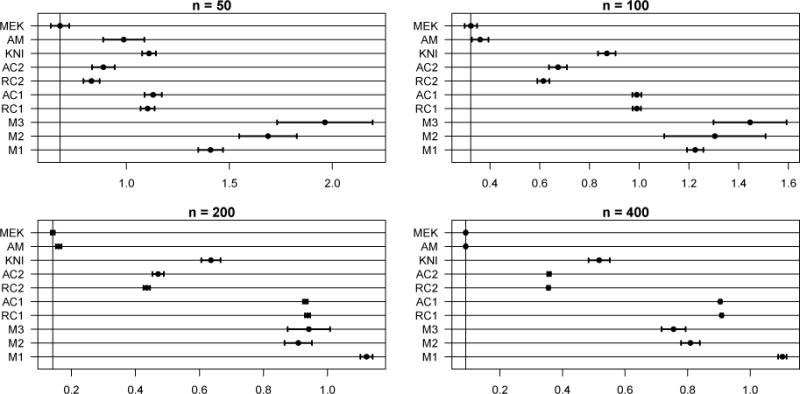
AISEs for Model 3. Note the scale differences. Out of the 400 MC samples, 2 and 1 AISE outlier(s) are omitted from M3 and M2, respectively.

Model 4

This example uses the functions Z(⋅) and ϕ(⋅) taken from Friedman (1991); see Section 4.1 for a description. We add a variable selection aspect to the original simulation in Friedman by including six additional irrelevant covariates having iid U(0, 1) distributions, for a total of ten covariates. We also increase the residual error so the model R² is 0.75 (lowering the signal-to-noise ratio from 9 to 3) to match Models 1–3. From Section 4.1, we know that X₁ in Z(⋅) and X₄ in both models are essentially irrelevant predictors, and we consider them as irrelevant when calculating selection error rates.

Selection error rates for Model 4 are displayed in Table 4. Average integrated squared errors (AISE) are shown in Figure 7; AISEs too large to display in the plot windows are indicated by dashed horizontal lines.

Table 4.

Selection error rates for Model 4, with X₁ in Z(⋅) and X₄ classified irrelevant. MC standard errors for all cells ≤ 0.04.

	Error	MEK	AM	KNI	AC2	RC2	AC1	RC1	M2	M1
Z(⋅) n = 100	Type I Type II	0.03 0.00	0.49 0.00	0.03 0.48	0.49 0.02	0.05 0.00	0.08 0.09	0.15 0.00	0.60 0.00	0.67 0.00
Z(⋅) n = 400	Type I Type II	0.01 0.00	0.50 0.00	0.01 0.50	0.04 0.00	0.03 0.00	0.01 0.00	0.13 0.00	0.58 0.00	0.63 0.00
ϕ(⋅) n = 100	Type I Type II	0.05 0.02	0.54 0.00	0.00 0.56	0.27 0.16	0.09 0.32	0.28 0.00	0.10 0.01	0.54 0.00	0.64 0.01
ϕ(⋅) n = 400	Type I Type II	0.00 0.00	0.51 0.00	0.12 0.26	0.21 0.01	0.01 0.06	0.18 0.00	0.04 0.00	0.37 0.00	0.59 0.00

Figure 7.

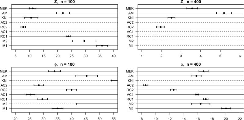
AISEs for Model 4; units for Z(⋅) plots are 10³ and units for ϕ(⋅) plots are 10⁻³. Note the scale differences. Dashed lines indicate methods with AISEs too large to display.

Although MEKRO (MEK) exhibits very good selection rates for both sample sizes and response functions, it falls short in predictions to COSSO (RC and AC variants) depending on the setup. MEKRO suffers from the same boundary effect problems as the Nadaraya-Watson estimator (Scott, 1992). Both Z(∙) and ϕ(∙) vary rapidly near their boundary points (see Friedman (1991) for surface plots), inflating MEKRO’s prediction error rate. Examining a plot of Z(⋅, X₂, X₃, ⋅) (not shown) reveals that much of the surface variation is attributed to the X₂X₃ interaction. The additive COSSOs (RC1, AC1) cannot pick this effect out and predict poorly. When n = 100, the weights in two-way interaction ACOSSO (AC2) reduce the component penalties too far and irrelevant covariates are overly selected. Even in the larger sample size, when two-way interaction ACOSSO selects well, the weights impart too much component variation leading to poor predictions. The two-way interaction COSSO (RC2) performs well.

Model 5

For this model, data are generated from the deterministic function describing the kinematics of the Puma 560 robotic arm (the data are available from the DELVE¹ data repository; see www.cs.toronto.edu/~delve/data/pumadyn/desc.html² for details). The arm has six independently-operating joints. The goal is to estimate the linear acceleration in Joint 3, given the position, velocity, and torque of all of the joints. This example sets several parameters to zero to reduce the number of active covariates to eight. We append four irrelevant covariates to judge selection performance. DELVE adds noise to both the input parameters and the response in two levels, medium and high (‘pumadyn-8nm’ and ‘pumadyn-8nh’ respectively in DELVE). We cannot estimate predictor effect sizes because we do not have access to the data generating function.

There are N = 8192 observations available. Because we do not have the luxury of generating a test data set, we randomly select n training observations without replacement and use the remaining N − n samples to estimate the conditional squared prediction error, $\widehat{\mathrm{SPE}}={(N-n)}^{-1}{\displaystyle {\sum }_{i=1}^{N-n}{\{Y_i-\widehat{g}({\mathit{x}}_i)\}}^2}$. The sampling process is repeated 100 times, and the average of the $\widehat{\mathrm{SPE}}$ values, the ASPE, estimates the squared prediction error. We report results for training sizes of n = 100, 200.

ASPEs are given in Figure 8 and main effect selection rates, the proportion of main effects selected out of the 100 MC samples, are given in Table 5. Note that these are not selection errors as shown on the previous tables. Interaction effect selection rates are excluded because we do not know which interactions are weak and effectively irrelevant. Table 5 shows selection rates averaged over the four simulations (main effect selection rates are similar across the four simulations). The ‘IRR’ row is the average inclusion rate for the four irrelevant covariates that are extraneous to the original data set.

Figure 8.

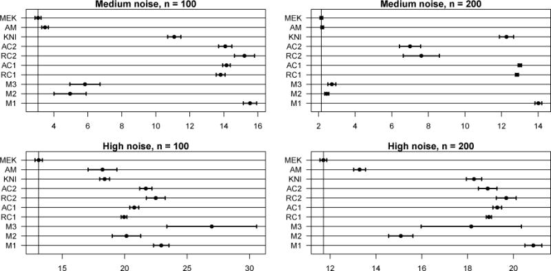
ASPEs (average squared prediction errors) for Model 5. Note the scale differences. Out of the 400 MC samples, 3 ASPE outliers are omitted from both M3 and M2.

Table 5.

Main effect selection rates (not errors) for Model 5, averaged over the four simulation settings. The IRR row is the average selection rate for the four irrelevant predictors that were independently generated. MC standard errors for all cells ≤ 0.03.

	MEK	AM	KNI	AC2	RC2	AC1	RC1	M3	M2	M1
X1	0.01	0.49	0.62	0.41	0.44	0.22	0.09	0.47	0.29	0.01
X2	1.00	1.00	1.00	1.00	1.00	1.00	1.00	1.00	1.00	1.00
X3	1.00	1.00	1.00	1.00	1.00	1.00	0.99	1.00	0.99	0.97
X4	0.01	0.52	0.66	0.50	0.52	0.25	0.09	0.48	0.30	0.01
X5	0.01	0.55	0.66	0.66	0.65	0.24	0.09	0.44	0.29	0.01
X6	0.01	0.50	0.60	0.44	0.47	0.26	0.10	0.48	0.32	0.01
X7	0.01	0.48	0.62	0.39	0.44	0.23	0.09	0.46	0.31	0.01
X8	0.01	0.48	0.69	0.45	0.45	0.24	0.09	0.47	0.30	0.01
IRR	0.01	0.51	0.65	0.41	0.44	0.25	0.10	0.16	0.12	0.01

MEKRO includes X₂ and X₃, the positions of the second and third joints, on every replicate, and excludes every other variable at a very high rate. Additive MARS (M1) shows a very similar selection performance. KNIFE, AMKR, and the four COSSO variants (KNI, AM, RC and AC) show generally higher selection rates for both active and irrelevant predictors, suggesting that the selection procedures are discriminating poorly. The two-way and three-way interaction MARS (M2 and M3) models show elevated active covariate selection rates, while keeping the irrelevant covariate selection rate low. Despite only selecting two of the eight active covariates, MEKRO has a better prediction rate than any other method, including the two MARS methods that show better covariate discrimination.

Goutte and Larsen (2000) benchmark AMKR (AM) against an artificial neural network (without ARD) and Gaussian process on the same Puma DELVE data sets, giving us indirect comparisons on prediction error. AMKR outperformed the artificial network, suggesting that MEKRO would do the same if ARD is not implemented. The Gaussian process generally predicted better than AMKR by 2–5% (quadratic loss comparison as a percentage) for n near 100 or 200, indicating that MEKRO would enjoy the best prediction rates in the high noise scenario and similar prediction rates in the medium noise scenario.

Prostate Data Example

The data are from a study of 97 men with prostate cancer (Stamey et al., 1989) and were used in the original LASSO paper (Tibshirani, 1996). The data contain the log level of a prostate-specific biomarker (response) along with eight other clinical measures (predictors): log cancer volume, log prostate weight, age, log benign prostatic hyperplasia amount, seminal vesicle invasion (binary), log capsular penetration, Gleason score, and percentage of Gleason scores equal to 4 or 5.

We evaluate the nonparametric methods by training on two-thirds of the data and evaluating the predictions on the remaining third. This process is repeated 100 times and the squared prediction errors are averaged. We also include LASSO, tuned with 10-fold cross-validation, and evaluate it in the same way.

The average squared prediction errors (ASPE) are given in Figure 9 and the selection rates (not errors) are given in Table 6. Predictions in the prostate data favor simpler methods as evidenced by LASSO and additive MARS (M1, versus M2 and M3, the higher-order MARS methods). Among the nonparametric methods, MEKRO (MEK) and KNIFE (KNI) have the smallest average model size while maintaining a low prediction error and high correlation with LASSO (LAS) selection. The MARS methods overfit and have high prediction errors. All COSSO (RC and AC variants) methods perform similarly in terms of prediction, selection, and correlation with LASSO, and have both higher average model sizes and higher prediction errors than MEKRO.

Figure 9.

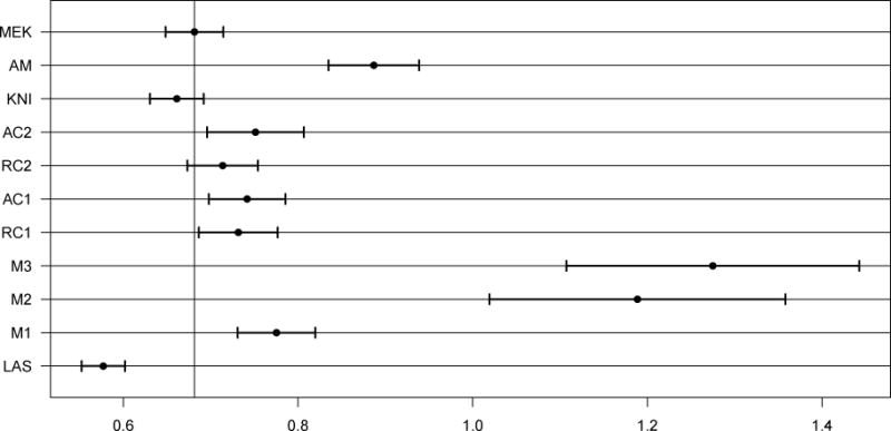
ASPEs (average squared prediction errors) for the prostate data. Out of the 100 MC samples, 2 and 4 ASPE outliers are omitted from M3 and M2, respectively.

Table 6.

Main effect selection rates (not errors) for the prostate data. ‘Avg Model’ is the method’s average model size; ‘Corr’ is the selection rate correlation of each method with LAS. MC standard errors for all selection rates ≤ 0.07 and all average model sizes ≤ 0.55.

	MEK	AM	KNI	AC2	RC2	AC1	RC1	M3	M2	M1	LAS
X1	1.00	1.00	0.98	1.00	1.00	1.00	1.00	1.00	1.00	1.00	1.00
X2	0.78	0.99	0.76	0.71	0.77	0.95	0.96	0.99	0.98	1.00	1.00
X3	0.01	0.46	0.00	0.44	0.52	0.53	0.54	0.86	0.83	0.96	0.48
X4	0.29	0.75	0.19	0.44	0.46	0.76	0.70	0.84	0.82	0.91	0.75
X5	0.64	0.91	0.82	0.94	0.90	0.99	0.97	0.82	0.84	0.97	1.00
X6	0.01	0.58	0.01	0.33	0.12	0.39	0.40	0.81	0.80	0.89	0.21
X7	0.14	0.71	0.25	0.21	0.17	0.30	0.51	0.26	0.32	0.27	0.39
X8	0.10	0.52	0.11	0.41	0.42	0.48	0.53	0.71	0.73	0.90	0.65
Avg Model	2.97	5.92	3.12	4.48	4.36	5.40	5.61	6.29	6.32	6.90	5.48
Corr	0.89	0.80	0.86	0.87	0.93	0.94	0.96	0.55	0.60	0.51	1.00

5 Asymptotic Results

Consider the model Y = g(X) + ε, where $\text{Var}(\epsilon |\mathit{X})={\sigma }_{\epsilon }^2$ and g(x) = E(Y|X = x). Define the important predictor set $\mathcal{I}=\{j:X_j\text{is important in}g(\cdot )\}$ and so its complement ${\mathcal{I}}^c$ is the set of unimportant predictors. We argue in online Appendix B that we can generally expect, if τ → ∞ and satisfies ${\tau }^{\left|\mathcal{I}\right|+4}/n\to 0$ and τ^p log(n)/n → 0 as n → ∞, then the maximizer $\widehat{\mathit{\lambda }}$ of (2) subject to the constraints (4) satisfies $\widehat{{\lambda }_j}\to \infty$ and $\widehat{{\lambda }_{j^{\prime }}}\to 0$ in probability for $j\in \mathcal{I}$ and $j^{\prime }\in {\mathcal{I}}^c$, i.e., the MEKRO asymptotically discriminates important from unimportant predictors and achieves variable selection consistency.

6 Discussion

We developed a new method for performing simultaneous variable and bandwidth selection in nonparametric regression using the SWW (Stefanski et al., 2014) paradigm. The resulting method is kernel regression with a novel bandwidth estimator (MEKRO). The bandwidth selection strategy is such that certain bandwidths are set to infinity (inverse bandwidth of 0), thereby allowing for complete removal of variables from the model. It is also attractive in that it does not require a complexity truncation and can fit models with many interactions. Simulation studies show that MEKRO is a viable option for selection and prediction generally, and especially useful when the underlying model is nonlinear with complex interactions.

Measurement error model selection likelihoods in linear models share a connection with LASSO, and also perform well when used for nonparametric classification. Although current implementations of the SWW approach focus on estimators with closed-form selection likelihoods, the favorable performance of such estimators suggests further study of selection likelihoods in more complex cases.

Despite the advantages of the new selection strategy, MEKRO is a local-constant kernel regression estimator and does not avoid the known drawbacks of the method. Future work will address boundary corrections, and an adaptive-bandwidth MEKRO that we suspect will boost prediction performance. Also, the scope of MEKRO can be expanded by adapting an ordinal kernel analogous to that in Racine and Li (2004) or allowing different response types. It is likely that major computational gains can be realized by implementing an approximate MEKRO that takes advantage of binning.

Appendix

A MEKRO Selection Likelihood Derivation

Stefanski et al. (2014) proposed a four-step approach for building a measurement error model (MEM) selection likelihood from any ‘traditional’ likelihood of covariates and a response. The measurement error kernel regression operator (MEKRO) is derived from these steps, and so they are included below for completeness. See Stefanski et al. (2014) for comprehensive details on the motivation for MEM selection likelihoods, their relationship to LASSO, and an application that yields a nonparametric classifier that performs variable selection. Let diag{a} be a diagonal matrix with the vector a on the diagonal. The MEM selection likelihood construction proceeds in four basic steps:

• S1. Start with an assumed ‘true’ likelihood for $\{{\left({\mathit{X}}_i,Y_i\right)}_{i=1}^n\}$, denoted ${\widehat{L}}_{\mathrm{TRUE}}(\mathit{\theta })$, where θ could be finite (parametric) or infinite dimensional (nonparametric).

• S2. Construct the associated measurement error model likelihood under the ‘false’ assumption that the components of X are measured with independent error. That is, assume that W is observed in place of X where $\mathit{W}|\mathit{X}\sim \mathrm{N}(\mathit{X},\mathrm{diag}\{{\mathit{\sigma }}_u^2\})$ with ${\mathit{\sigma }}_u^2=({\sigma }_{u,1}^2,\dots ,{\sigma }_{u,p}^2)$. The resulting likelihood depends on θ and ${\mathit{\sigma }}_u^2$ and is denoted $L_{\mathrm{MEM}}(\mathit{\theta },{\mathit{\sigma }}_u^2)$. Note that even though $L_{\mathrm{MEM}}(\mathit{\theta },{\mathit{\sigma }}_u^2)$ is derived under a measurement error model assumption, it is calculated from the error-free data $\{{\left({\mathit{X}}_i,Y_i\right)}_{i=1}^n\}$.

• S3. Replace θ in $L_{\mathrm{MEM}}(\mathit{\theta },{\mathit{\sigma }}_u^2)$ with an estimate, $\widehat{\mathit{\theta }}$, resulting in the pseudo-profile likelihood ${\widehat{L}}_{\mathrm{pMEM}}({\mathit{\sigma }}_u^2)=L_{\mathrm{MEM}}(\widehat{\mathit{\theta }},{\mathit{\sigma }}_u^2)$. Note that $\widehat{\mathit{\theta }}$ is an estimator for θ calculated from the observed data without regard to the ‘false’ measurement error assumption, e.g., $\widehat{\mathit{\theta }}$ could be the maximum likelihood estimator from ${\widehat{L}}_{\mathrm{TRUE}}(\mathit{\theta })$.

• S4. Reexpress the pseudo-profile likelihood ${\widehat{L}}_{\mathrm{pMEM}}({\mathit{\sigma }}_u^2)$ in terms of precision (or square-root precision) λ =(λ₁, …, λ_p) where ${\lambda }_j=1/{\sigma }_{u,j}^2$ (or λ_j = 1/σ_{u, j}), resulting in the MEM selection likelihood ${\widehat{L}}_{\mathrm{SEL}}(\mathit{\lambda })$.

${\widehat{L}}_{\mathrm{SEL}}(\mathit{\lambda })$ is maximized subject to: λ_j ≥ 0, j = 1, …, p; and ${\displaystyle {\sum }_{j=1}^p{\lambda }_j=\tau }$. Setting the tuning parameter τ < ∞ in the latter constraint ensures that the harmonic mean of the measurement error standard deviations is p/τ > 0. This is how the approach forces ‘false’ measurement error into the likelihood.

We show that application of the measurement error model selection likelihood approach to nonparametric regression results in MEKRO. Consider the quadratic loss pseudo-likelihood (negative loss) functional,

$${\widehat{L}}_{\mathrm{TRUE}}(F_{Y,\mathit{X}})=-\frac{1}{n}{\displaystyle \sum _{i=1}^n{\{Y_i-g_{Y|\mathit{X}}({\mathit{X}}_i)\}}^2},$$

where

$$g_{Y|\mathit{X}}(\mathit{X})=\frac{{\displaystyle \int y{f}_{Y,\mathit{X}}(y,\mathit{x})dy}}{{\displaystyle \int f_{Y,\mathit{X}}(y,\mathit{x})dy}},$$

and f_Y,X(y, x) = ∂^p+1/(∂y∂x₁ ⋯ ∂x_p)F_Y,X(y, x). Note that F_Y,X(⋅, ⋅) plays the role of θ in the four-step algorithm. Assume that W_i is observed instead of X_i, where W_i = X_i + diag{σ_u} U_i and ${\mathit{U}}_i\stackrel{\text{iid}}{\sim }{\mathrm{N}}_p(\mathbf{0},{\mathit{I}}_p)$ and is independent of all other data, to give

$$L_{\mathrm{MEM}}(F_{Y,\mathit{W},}{\mathit{\sigma }}_u^2)=-\frac{1}{n}{\displaystyle \sum _{i=1}^n{\{Y_i-g_{Y|\mathit{W}}({\mathit{X}}_i)\}}^2}$$

where g_Y|W(∙) depends on σ_u implicitly. We derive an expression for g_Y|W(⋅); observe,

$$\begin{array}{l}{f}_{Y,\mathit{W}}(y,\mathit{w})=\frac{{\partial }^{p+1}}{\partial y\partial w_1\cdots \partial w_p}P(Y\le y,\mathit{W}\le \mathit{w})\\ ={\displaystyle \int f_{Y,\mathit{X}}(y,\mathit{w}-\mathrm{diag}\{{\mathit{\sigma }}_u\}\mathit{u}){\displaystyle \prod _{j=1}^p\varphi (u_j)d\mathit{u}}},\end{array}$$

where the interchange of differentiation and integration is justified for the Gaussian product kernel and many others. Consequently,

$$\begin{array}{l}{g}_{Y|\mathit{W}}(\mathit{x})=E(Y|\mathit{W}=\mathit{x})\\ ={\displaystyle \int y{f}_{Y|\mathit{W}}(y|\mathit{x})dy}\\ =\frac{{\displaystyle \int y}{\displaystyle \int f_{Y,\mathit{X}}(y,\mathit{x}-\mathrm{diag}\{{\mathit{\sigma }}_u\}\mathit{u}){\displaystyle {\prod }_{j=1}^p\varphi (u_j)}d\mathit{u}dy}}{{\displaystyle \iint f_{Y,\mathit{X}}(y,\mathit{x}-\mathrm{diag}\{{\mathit{\sigma }}_u\}\mathit{u}){\displaystyle {\prod }_{j=1}^p\varphi (u_j)}d\mathit{u}dy}}\\ =\frac{{\displaystyle \int y}{\displaystyle \int f_{Y,\mathit{X}}(y,\mathit{t}){\displaystyle {\prod }_{j=1}^p\varphi \{(x_j-t_j)/{\sigma }_j\}{({\sigma }_{u,j})}^{-1}}d\mathit{t}dy}}{{\displaystyle \iint f_{Y,\mathit{X}}(y,\mathit{t}){\displaystyle {\prod }_{j=1}^p\varphi \{(x_j-t_j)/{\sigma }_{u,j}\}{({\sigma }_{u,j})}^{-1}}d\mathit{t}dy}}\\ =\frac{{\displaystyle \iint y{\displaystyle {\prod }_{j=1}^p\varphi \{(x_j-t_j)/{\sigma }_{u,j}\}{F}_{Y,\mathit{X}}}(dy,d\mathit{t})}}{{\displaystyle \iint {\displaystyle {\prod }_{j=1}^p\varphi \{(x_j-t_j)/{\sigma }_{u,j}\}{F}_{Y,\mathit{X}}}(dy,d\mathit{t})}}\end{array}$$

after noting the change of variables u_j = (x_j − t_j)/σ_u,j and that ϕ(∙) is the standard normal pdf. Step S3 in the four-step algorithm calls for estimation of θ, which in this setting means estimation of F_Y,X(⋅,⋅). The empirical cdf is substituted to give ${\widehat{L}}_{\mathrm{pMEM}}$ (not shown). Finally, the measurement error standard deviations are parameterized as inverse standard deviations (S4) to produce the MEM selection likelihood,

$${\widehat{L}}_{\mathrm{SEL}}(\mathit{\lambda })=-\frac{1}{n}{\displaystyle \sum _{i=1}^n{\{Y_i-\widehat{g}({\mathit{X}}_i,\mathit{\lambda })\}}^2},$$

where,

$$\widehat{g}({\mathit{X}}_i,\mathit{\lambda })=\frac{{\displaystyle {\sum }_{k=1}^n{Y}_k{\displaystyle {\prod }_{j=1}^p\exp \{-{\lambda }_j^2{(X_{i,j}-X_{k,j})}^2/2\}}}}{{\displaystyle {\sum }_{k=1}^n{\displaystyle {\prod }_{j=1}^p\exp \{-{\lambda }_j^2{(X_{i,j}-X_{k,j})}^2/2\}}}}.$$

There is now an explicit dependence of $\widehat{g}(\cdot )$ on λ that have entered the selection likelihood as inverse smoothing bandwidth parameters.

B Asymptotic Selection Consistency

Using a mix of known results, detailed derivations, and heuristics, we explain the apparent large-sample selection consistency manifest in our simulation studies. For the multivariate Nadaraya-Watson estimator, we denote the smoothing bandwidth for predictor j by h_j and h = (h₁, …, h_p)^T. In Section 2.1 of Li and Racine (2007), the pointwise asymptotic bias and variance are rigorously established for the multivariate Nadaraya-Watson estimator, $\widehat{g}(\mathit{x},1/\mathit{h})-g(\mathit{x})=O_p\left({\displaystyle {\sum }_{j=1}^p{h}_j^2+{\left(n{\displaystyle {\prod }_{j=1}^p{h}_j}\right)}^{-1/2}}\right)$, where 1/h = (1/h₁, …, 1/h_p)^T.

In MEKRO, one maximizes the MEM selection likelihood (2) subject to constraint (4), which is equivalent to minimizing the fitted mean squared error $-{\widehat{L}}_{\mathrm{SEL}}(\mathit{\lambda })$ subject to this constraint. In order to study the asymptomatic properties for the optimizer, we need to characterize the asymptotic behavior of $-{\widehat{L}}_{\mathrm{SEL}}(\mathit{\lambda })$ in a similar format as Lemma A1 in Wu and Stefanski (2015). Their Lemma A1 follows from technical proofs of Fan and Jiang (2005), whose techniques can be used to extend the pointwise asymptotic results of Li and Racine (2007) and argue that under regularity conditions of the type in Fan and Jiang (2005), if bandwidths satisfy h_j ⟶ 0 for j = 1, …, p and $n{\displaystyle {\prod }_{j=1}^p{h}_j/\log (n)\to \infty }$ as n → ∞, it holds that,

$$\frac{1}{n}{\displaystyle \sum _{i=1}^n{\{Y_i-\widehat{g}({\mathit{X}}_i,1/\mathit{h})\}}^2}={\sigma }_{\epsilon }^2+O_p\left({\displaystyle \sum _{j=1}^p{h}_j^4+{\left(n{\displaystyle \prod _{j=1}^p{h}_j}\right)}^{-1}}\right).$$ (12)

In (12), the smoothing bandwidth for each predictor shrinks to zero as the sample size diverges to infinity. Yet, it is well known that the use of a small bandwidth in local polynomial smoothing reduces approximation bias in Taylor-series expansions and thus also estimation bias (Fan and Gijbels, 1996). This is echoed in the asymptotic bias formula that appears below Equation (2.8) on page 62 of Li and Racine (2007), where it is explicitly shown that the bias corresponding to predictor j has a factor of $2\frac{\partial f(\mathit{x})}{\partial x_j}\frac{\partial g(\mathit{x})}{\partial x_j}+f(\mathit{x})\frac{{\partial }^{2}g(\mathit{x})}{\partial x_j^2}$, where f (∙) is the density of X. If $j\notin \mathcal{I}$, the index set of important predictors in g(⋅), this factor is equal to zero because $\frac{\partial g(\mathit{x})}{\partial x_j}=0$ and $\frac{{\partial }^{2}g(\mathit{x})}{\partial x_j^2}=0$ when predictor j is not important. Thus in a Taylor-series expansion of the multivariate Nadaraya-Watson estimator, predictor j does not contribute to the approximate bias if $j\notin \mathcal{I}$ and the corresponding smoothing bandwidth is not required to shrink to zero as the sample size diverges. This suggests that (12) can be further refined to show that if bandwidths satisfy h_j → 0 for $j\in \mathcal{M}$, h_j′ ≥ c₀ > 0 for $j^{\prime }\in {\mathcal{M}}^c$ and some c₀ > 0, and $n{\displaystyle {\prod }_{j\in \mathcal{M}}{h}_j/\log (n)\to \infty }$ as n → ∞ for a set $\mathcal{M}$ satisfying $\mathcal{I}\subseteq \mathcal{M}\subseteq \{1,\dots ,p\}$, we have,

$$\frac{1}{n}{\displaystyle \sum _{i=1}^n{\{Y_i-\widehat{g}({\mathit{X}}_i,1/\mathit{h})\}}^2}={\sigma }_{\epsilon }^2+O_p\left({\displaystyle \sum _{j\in \mathcal{M}}{h}_j^4+}{\left(n{\displaystyle \prod _{j\in \mathcal{M}}{h}_j}\right)}^{-1}\right).$$ (13)

To gain insight, we now consider a deterministic version of the O_p in (13) with transformation t_j = 1/h_j. For a set $\mathcal{M}$ satisfying $\mathcal{I}\subseteq \mathcal{M}\subseteq \{1,\dots ,p\}$ and n large enough, denote ${\widehat{\mathit{t}}}_{\mathcal{M}}={({\widehat{t}}_j,j\in \mathcal{M})}^T$ as the minimizer of

$${\displaystyle \sum _{j\in \mathcal{M}}{t}_j^{-4}}+n^{-1}{\displaystyle \prod _{j\in \mathcal{M}}{t}_j},\text{subject to}{t}_j\ge \log (n),j\in \mathcal{M},\text{and}{\displaystyle \sum _{j\in \mathcal{M}}{t}_j=T_n>0},$$ (14)

where T_n satisfies T_n → ∞ and $T_n^p\log (n)/n\to 0$ as n → ∞. Here the constraint t_j ≥ log(n) guarantees that h_j = 1/t_j converges to zero as required by (13), where log(n) can be replaced by any sequence that slowly diverges to infinity. Note that the optimization problem is symmetric in t_j and thus it follows that the minimizer is given by ${\widehat{t}}_j=T/|\mathcal{M}|$, $j\in \mathcal{M}$, and the corresponding objective function takes value ${\left|\mathcal{M}\right|}^5/T^4+{(T/\left|\mathcal{M}\right|)}^{\left|\mathcal{M}\right|}/n$, where $\left|\mathcal{M}\right|$ denotes the cardinality of set $\mathcal{M}$ and T ≡ T_n. By treating $\left|\mathcal{M}\right|$ as a continuous variable and examining the first derivative with respect to $\left|\mathcal{M}\right|$, we conclude ${\left|\mathcal{M}\right|}^5/T^4+{(T/\left|\mathcal{M}\right|)}^{\left|\mathcal{M}\right|}/n$ is monotonically increasing in $\left|\mathcal{M}\right|$ if $0<\left|\mathcal{M}\right|<T/e$. We next appeal to these results to assert that ${\widehat{\lambda }}_j\to \infty$ for $j\in \mathcal{I}$ and ${\widehat{\lambda }}_j\to 0$ for $j\in {\mathcal{I}}^c$

Selection consistency of MEKRO

We first argue that ${\widehat{\lambda }}_j\to \infty$ in probability for $j\in \mathcal{I}$ as n → ∞. According to (13), $-{\widehat{L}}_{\mathrm{SEL}}(\mathit{\lambda })$ converges to ${\sigma }_{\epsilon }^2$ as long as the smoothing parameters of all important predictors shrink to zero as the sample size diverges to infinity. On the other hand, according to the proof of the asymptotic bias and variance in Li and Racine (2007), the multivariate Nadaraya-Watson estimator is not consistent if smoothing bandwidths of any important predictor do not shrink to zero as the sample size diverges to infinity. Correspondingly, $-{\widehat{L}}_{\mathrm{SEL}}(\mathit{\lambda })$ will converge to ${\sigma }_{\epsilon }^2$ plus a squared bias term that does not shrink to zero asymptotically. Recall that λ_j is the reciprocal smoothing bandwidth and $\widehat{\mathit{\lambda }}$ is the solution that minimizes $-{\widehat{L}}_{\mathrm{SEL}}(\mathit{\lambda })$ subject to subject to constraint (4), thus, minimization will not lead to ${\widehat{\lambda }}_j\nrightarrow \infty$ for $j\in \mathcal{I}$ as the corresponding limit of the objective function is larger than ${\sigma }_{\epsilon }^2$, which is attainable. Consequently, we have ${\widehat{\lambda }}_j\to \infty$ in probability for any $j\in \mathcal{I}$ as n → ∞.

Consistency of MEKRO is achieved provided ${\widehat{\lambda }}_j\to 0$ in probability for $j\in {\mathcal{I}}^c$, which we now argue. First we show ${\widehat{\lambda }}_j\nrightarrow \infty$ in probability for $j\in {\mathcal{I}}^c$. The MEKRO solution converges to ${\sigma }_{\epsilon }^2$ with an asymptotic rate of $O_p\left({\displaystyle {\sum }_{j\in \mathcal{M}}{h}_j^4+{\left(n{\displaystyle {\prod }_{j\in \mathcal{M}}{h}_j}\right)}^{-1}}\right)$ according to (13). The deterministic version of this rate is a monotonically increasing function of the cardinality $\left|\mathcal{M}\right|$ of the set of predictors whose corresponding λ_j → ∞ by noting λ_j = 1/h_j. Thus, the MEKRO solution must satisfy ${\widehat{\lambda }}_j\nrightarrow \infty$ in probability for $j\in {\mathcal{I}}^c$ because minimization favors a faster convergence rate, and so $\mathcal{M}=\mathcal{I}$. Further, ${\widehat{\lambda }}_j$ has the same order as τ for $j\in \mathcal{I}$.

It remains to argue that ${\widehat{\lambda }}_j$ converging to a positive constant in probability for $j\in {\mathcal{I}}^c$ is not favored. Denote ${\widehat{\mathcal{A}}}_{\infty }=\{j:{\widehat{\lambda }}_j\to \infty \text{in probability as}n\to \infty \}$, ${\widehat{\mathcal{A}}}_0=\{j:{\widehat{\lambda }}_j\to 0\text{in probability as}n\to \infty \}$, and $\begin{array}{l}{\widehat{\mathcal{A}}}_1=\{1,\dots ,p\}\backslash ({\widehat{\mathcal{A}}}_0\cup {\widehat{\mathcal{A}}}_{\infty })\\ \end{array}$. From the above argument we have ${\widehat{\mathcal{A}}}_{\infty }=\mathcal{I}$. Then, for $j\in {\widehat{\mathcal{A}}}_1$, the sequence ${\widehat{\lambda }}_j$ is asymptotically bounded away from both 0 and ∞. We assume without loss of generality that ${\widehat{\lambda }}_j\to c_j$ in probability for $j\in {\widehat{\mathcal{A}}}_1$ and some 0 < c_j < ∞; otherwise, we consider any convergent subsequence of ${\widehat{\lambda }}_j$. Thus $\tau -{\displaystyle {\sum }_{j\in {\widehat{\mathcal{A}}}_{\infty }}{\widehat{\lambda }}_j\to {\displaystyle {\sum }_{j^{\prime }\in {\widehat{\mathcal{A}}}_1}{c}_{j^{\prime }}}}$ in probability. Now consider an alternative solution sequence ${\stackrel{\sim }{\lambda }}_j={\widehat{\lambda }}_j\tau /(\tau -{\displaystyle {\sum }_{j^{\prime }\in {\mathcal{I}}^c}{\widehat{\lambda }}_{j^{\prime }}})$ for $j\in \mathcal{I}$ and ${\stackrel{\sim }{\lambda }}_{j^{\prime }}=0$ for $j^{\prime }\in {\mathcal{I}}^c$. Equation (13) gives ${\sigma }_{\epsilon }^2+O_p({\displaystyle {\sum }_{j\in \mathcal{I}}{\widehat{\lambda }}_j^{-4}}+{\displaystyle {\prod }_{j\in \mathcal{I}}{\widehat{\lambda }}_j}/n)$ for the solution ${\widehat{\lambda }}_j$ and ${\sigma }_{\epsilon }^2+O_p(b^{-4}{\displaystyle {\sum }_{j\in \mathcal{I}}{\widehat{\lambda }}_j^{-4}+b^{\left|\mathcal{I}\right|}}{\displaystyle {\prod }_{j\in \mathcal{I}}{\widehat{\lambda }}_j}/n)$ for the alternative solution ${\stackrel{\sim }{\lambda }}_j$, where $b=\tau /(\tau -{\displaystyle {\sum }_{j^{\prime }\in {\mathcal{I}}^c}{\widehat{\lambda }}_{j^{\prime }}})\ge 1$. Note that b = 1 iff ${\mathcal{I}}^c=\varnothing$ in which case all ${\widehat{\lambda }}_j\to \infty$ as desired; we henceforth assume at least one predictor is unimportant and thus b > 1. We argued above that ${\widehat{\lambda }}_j$ has the same order as τ for $j\in \mathcal{I}$ and because τ → ∞ satisfies ${\tau }^{\left|\mathcal{I}\right|+4}/n\to 0$ as n → ∞ by assumption, the asymptotic bias $O_p({\displaystyle {\sum }_{j\in \mathcal{I}}{\widehat{\lambda }}_j^{-4}})$ dominates the asymptotic variance $O_p({\displaystyle {\prod }_{j\in \mathcal{I}}{\widehat{\lambda }}_j/n})$. The alternative solution ${\stackrel{\sim }{\lambda }}_j$ will be favored in the process of minimizing the fitted mean squared error because b > 1 and thus the leading term of $O_p(b^{-4}{\displaystyle {\sum }_{j\in \mathcal{I}}{\widehat{\lambda }}_j^{-4}+b^{\left|\mathcal{I}\right|}{\displaystyle {\prod }_{j\in \mathcal{I}}{\widehat{\lambda }}_j}}/n)$ has a smaller constant than that of $O_p({\displaystyle {\sum }_{j\in \mathcal{I}}{\widehat{\lambda }}_j^{-4}+{\displaystyle {\prod }_{j\in \mathcal{I}}{\widehat{\lambda }}_j}}/n)$ even though they share the same asymptotic rate. This implies ${\widehat{\mathcal{A}}}_1=\varnothing$ and ${\widehat{\mathcal{A}}}_0={\mathcal{I}}^c$, completing the argument for every convergent subsequence of ${\widehat{\lambda }}_j$ and thus ${\widehat{\lambda }}_j$ in general.

C Numerical Study with Gaussian X

We explore MEKRO’s performance when X follows a Gaussian distribution to address a concern from reviewers that it may greatly underperform without uniform data. We copied Model 2 from Section 4.2, but with X drawn from N(0, 1) such that Corr(X) has an AR(1) structure with ρ = 0.5. To generate the predictor matrix X of stacked predictor vectors X^T, we generate a n × p matrix Z with each element iid N(0, 1) and define X = ZΣ where Σ^TΣ is the population AR(1) correlation matrix with ρ = 0.5. The predictors are scaled to be in [0, 1] to generate Y_i, i = 1, …, n, then scaled to have mean 0 and unit variance. Recall that Y is generated according to g(X) = sin{2π(X₁+X₂)/(1+X₃)} so that there are three active and seven irrelevant predictors. The predictor effect sizes are (1.00, 1.00, 0.32) for (X₁, X₂, X₃) and 0 for X₄ through X₁₀.

The average integrated squared errors (AISE) and selection errors for Model 2 with Gaussian X are shown in Figure 10 and Table 7, respectively. MEKRO (MEK) does not do as well with prediction in this scenario. Gaussian data are spread too thinly near the boundaries to give MEKRO good surface estimates; see Section 4.2, Model 4 for more details. However, MEKRO maintains superior selection performance when compared to all other methods at n ≥ 100 and achieves perfect selection at n = 400. The additive COSSO (RC1) that is similar to MEKRO for selection in Model 2 at n = 400 falls short with Gaussian X by frequently failing to include the weak predictor, X₃. Adding a boundary correction to boost MEKRO’s prediction performance is part of future work.

Table 7.

Selection error rates for the model in Appendix C. MC standard errors for all cells ≤ 0.03.

	Error	MEK	AM	KNI	AC2	RC2	AC1	RC1	M3	M2	M1
n = 50	Type I Type II	0.06 0.28	0.53 0.10	0.15 0.42	0.13 0.61	0.14 0.57	0.33 0.42	0.14 51	0.52 0.10	0.53 0.09	0.69 0.11
n = 100	Type I Type II	0.03 0.09	0.47 00	0.07 0.30	0.26 0.33	0.06 .46	0.27 0.22	0.04 0.32	0.51 0.00	0.50 0.01	0.60 0.05
n = 200	Type I Type II	0.01 0.02	0.44 0.00	0.06 0.28	0.23 0.31	0.05 0.42	0.33 0.11	0.02 0.24	0.41 0.00	0.39 0.00	0.59 0.03
n = 400	Type I Type II	0.00 0.00	0.45 0.00	0.11 0.13	0.23 0.0.35	0.03 0.08	0.29 0.20	0.01 0.00	0.26 0.00	0.27 0.03	0.56

References

- Allen GI. Automatic feature selection via weighted kernels and regularization. Journal of Computational and Graphical Statistics. 2013;22(2):284–299. [Google Scholar]
- Barron AR, Xiao X. Discussion: Multivariate adaptive regression splines. The Annals of Statistics. 1991;19(1):67–82. [Google Scholar]
- Fan J, Gijbels I. Local polynomial modelling and its applications: monographs on statistics and applied probability 66. Vol. 66. CRC Press; 1996. [Google Scholar]
- Fan J, Jiang J. Nonparametric inferences for additive models. Journal of the American Statistical Association. 2005;100(471):890–907. [Google Scholar]
- Friedman JH. Multivariate adaptive regression splines. The Annals of Statistics. 1991;19(1):1–67. [Google Scholar]
- Goutte C, Larsen J. Adaptive metric kernel regression. Journal of VLSI Signal Processing. 2000;26:155–167. [Google Scholar]
- Grandvalet Y, Canu S. Comments on “noise injection into inputs in back propagation learning”. Systems, Man and Cybernetics, IEEE Transactions on. 1995;25(4):678–681. [Google Scholar]
- Grandvalet Y, Canu S. Adaptive noise injection for input variables relevance determination. Artificial Neural Networks – ICANN ’97, 7th International Conference; Lausanne, Switzerland. October 8–10, 1997; 1997. pp. 463–468. Proceedings. [Google Scholar]
- Grandvalet Y, Canu S, Boucheron S. Noise injection: Theoretical prospects. Neural Computation. 1997;9(5):1093–1108. [Google Scholar]
- Hastie T, Tibshirani R, Friedman J. The Elements of Statistical Learning. 2nd Springer; 2009. [Google Scholar]
- Holmstrom L, Koistinen P. Using additive noise in back-propagation training. Neural Networks, IEEE Transactions on. 1992;3(1):24–38. doi: 10.1109/72.105415. [DOI] [PubMed] [Google Scholar]
- Hurvich CM, Simonoff JS, Tsai CL. Smoothing parameter selection in nonparametric regression using an improved akaike information criterion. Journal of the Royal Statistical Society. Series B (Statistical Methodology. 1998;60(2):271–293. [Google Scholar]
- Cook JR, S LA. Simulation-extrapolation estimation in parametric measurement error models. Journal of the American Statistical Association. 1994;89(428):1314–1328. [Google Scholar]
- Lafferty J, Wasserman L. Rodeo: Sparse, greedy nonparametric regression. The Annals of Statistics. 2008;36(1):28–63. [Google Scholar]
- Li Q, Racine J. Nonparametric Econometrics: Theory and Practice. Princeton University Press; 2007. [Google Scholar]
- Lin Y, Zhang HH. Component selection and smoothing in multivariate nonparametric regression. Annals of Statistics. 2006;34(5):2272–2297. [Google Scholar]
- Nadaraya EA. On estimating regression. Theory of Probability & Its Applications. 1964;9(1):141–142. [Google Scholar]
- Neal RM. Bayesian learning for neural networks. Springer-Verlag; 1996. [Google Scholar]
- Okazaki N. libLBFGS: a library of Limited-memory Broyden-Fletcher-Goldfarb-Shanno (L-BFGS) 2010 http://www.chokkan.org/software/liblbfgs/
- Racine J, Li Q. Nonparametric estimation of regression functions with both categorical and continuous data. Journal of Econometrics. 2004;119(4):99–130. [Google Scholar]
- Ravikumar P, Lafferty J, Liu H, Wasserman L. Sparse additive models. Journal of the Royal Statistical Society: Series B (Statistical Methodology) 2009;71(5):1009–1030. [Google Scholar]
- Scott DW. Multivariate density estimation: theory, practice, and visualization. John Wiley & Sons; 1992. [Google Scholar]
- Sietsma J, Dow RJ. Creating artificial neural networks that generalize. Neural Networks. 1991;4(1):67–79. [Google Scholar]
- Stamey T, Kabalin J, McNeal J, Johnstone I, Freiha F, Redwine E, Yang N. Prostate specific antigen in the diagnosis and treatment of adenocarcinoma of the prostate. ii. radical prostatectomy treated patients. Journal of Urology. 1989;141(5):1076–1083. doi: 10.1016/s0022-5347(17)41175-x. [DOI] [PubMed] [Google Scholar]
- Stefanski LA, Cook JR. Simulation-extrapolation: The measurement error jackknife. Journal of the American Statistical Association. 1995;90(432):1247–1256. [Google Scholar]
- Stefanski LA, Wu Y, White K. Variable selection in nonparametric classification via measurement error model selection likelihoods. Journal of the American Statistical Association. 2014;109(506):574–589. doi: 10.1080/01621459.2013.858630. [DOI] [PMC free article] [PubMed] [Google Scholar]
- Storlie CB, Bondell HD, Reich BJ, Zhang HH. Surface estimation, variable selection, and the nonparametric oracle property. Statistica Sinica. 2011;21(2):679–705. doi: 10.5705/ss.2011.030a. [DOI] [PMC free article] [PubMed] [Google Scholar]
- Tibshirani R. Regression shrinkage and selection via the lasso. Journal of the Royal Statistical Society. Series B (Methodological) 1996;58(1):267–288. [Google Scholar]
- Watson GS. Smooth regression analysis. Sankhyā: The Indian Journal of Statistics, Series A (1961–2002) 1964;26(4):359–372. [Google Scholar]
- Williams CK, Rasmussen CE. Gaussian processes for regression. MIT Press; 1996. [Google Scholar]
- Wu Y, Stefanski LA. Automatic structure recovery for additive models. Biometrika. 2015:asu070. doi: 10.1093/biomet/asu070. [DOI] [PMC free article] [PubMed] [Google Scholar]