

Abstract
This study describes the modifications made to the Goddard Earth Observing System (GEOS) Atmospheric Data Assimilation System (ADAS) to conserve atmospheric dry-air mass and to guarantee that the net source of water from precipitation and surface evaporation equals the change in total atmospheric water. The modifications involve changes to both the atmospheric model and the analysis procedure. In the model, sources and sinks of water are included in the continuity equation; in the analysis, constraints are imposed to penalize (and thus minimize) analysis increments of dry-air mass. Finally, changes are also required to the Incremental Analysis Update (IAU) procedure. The effects of these modifications are separately evaluated in free-running and assimilation experiments. Results are also presented from a multiyear reanalysis (Version 2 of the Modern Era Retrospective-Analysis for Research and Applications: MERRA-2) that uses the modified system.
Keywords: Renalysis, incremental analysis update, data assimilation, mass conservation
1. Introduction
All existing global atmospheric reanalyses done with NWP data assimilation systems attempt to analyze the total mass of the atmosphere from surface pressure observations. In doing so, they ignore the simple physical constraint that, to an excellent approximation, the atmosphere’s total ”dry-air mass” is invariant, and so, changes in total mass must be essentially the same as those in total water mass. Since the total water is also being analyzed, they are implicitly allowing spurious variations of dry-air mass.
Trenberth and Smith (2005) studied the changes in total mass, total water mass, and the implied change in dry-air mass produced by the ERA-40 reanalysis (Uppala et al. 2005). They used the results to estimate the total dry-air mass (5.1352 × 10¹⁸ kg or 983.05 hPa-equivalent), as well as the mean seasonal cycle of total mass. They also found significant variability in the implied dry-air mass. The seasonal range in water mass was 26% larger than that of total mass, and the two mass estimates were sufficiently uncorrelated over longer time scales that even crude estimates of inter-annual variability or trends would be problematic.
Berrisford et al. (2011) repeated this analysis for the newer ERA-Interim reanalysis (Dee et al. 2011) and found an improved situation, with a seasonal range of water mass that was only 15% larger than that of total mass. However, inter-annual and longer variations in dry-air mass were of comparable magnitude to those in ERA-40. In that article, they also addressed the question of whether reanalyses should impose a constraint limiting the variability of total dry-air mass, or continue making separate, inconsistent estimates of the total mass and total water. They argued that the analysis should provide an estimate of the dry-air mass, rather than simply assuming a value, and that the implied changes in dry-air mass are a useful measure of the accuracy of the analyses of surface pressure and atmospheric water.
To illustrate these issues, we show in Figs. 1–3 the different components of atmospheric mass as analyzed by ERA-Interim and NASA’s MERRA reanalysis (Rienecker et al. 2011). These results prompted us to reconsider the treatment of the mass balance in MERRA as we prepared for a new reanalysis (MERRA-2).
Figure 1.

Climatological seasonal cycle of the globally-integrated mass of dry air (orange) and of atmospheric water (blue) from MERRA and ERAInterim (in hPa of hydrostatic pressure).
Figure 3.

Monthly mean globally-integrated total water budget from the two reanalyses. Shown are the physical source terms (E − P), the analysis tendency, and the atmospheric water storage. Units are kg m−2 day−1.
In Fig. 1 we see that MERRA and ERA-Interim produced almost identical annual cycles of total water. The seasonal range of dry-air mass is comparable in the two, while the offset in dry-air mass could result from a difference as small as 1–2 m in the mean height of the topography used by the two models (Trenberth and Smith 2005).
Figure 2 shows monthly-mean anomalies from the mean seasonal cycle for total mass, total water, and dry-air mass. ERA-Interim has little or no trend in total water, but does show significant inter-annual fluctuations, the largest of which are clearly associated with El Niño events. Their total mass anomalies show some of these inter-annual variations, but are dominated by a period of low mass in the early 1980s and another of anomalously high mass between 1995 and 2005, with corresponding anomalies in the implied dry-air mass. The range of dry-air mass anomalies in ERA-Interim is 0.3 hPa, compared to a range of 0.1 hPa in total water. The situation in MERRA is somewhat different, but no better. The total mass shows some of the same features as ERA-Interim, but these are not matched as closely by the dry-air mass, due to a water vapor increase of roughly 0.15 hPa over the thirty years. Still, the magnitude of spurious anomalies in dry-air mass are similar in the two analyses.
Figure 2.
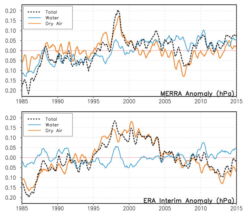
Globally-integrated monthly-mean mass anomalies from MERRA and ERA-Interim. Shown are the anomalies of total mass (black dots), as well as their decomposition into atmospheric water (blue) and dry air (orange) components (in hPa of hydrostatic pressure).
If we were to constrain the dry-air mass to be invariant during the reanalysis, the total water budget would completely determine fluctuations in total mass. Figure 3 shows the history of monthly means of the water budget for the current, unconstrained reanalyses. The budget is partitioned into three terms: the physical source term, evaporation minus precipitation (E − P); the analysis tendency; and the storage of water in the atmosphere. The storage term is dominated by the seasonal cycle and is much smaller than the other two, since it is strongly constrained by water vapor observations. Ideally, we would want the analysis increment to be small, as it is for ERA-Interim between 1992 and 1997, but this is more the exception than the rule. Analysis increments are generally large and subject to sudden changes, which previous studies have traced to changes in the observing system, particularly changes in SSM/I in 1992 (Trenberth and Fasullo 2013) and the introduction of ATOVS in 1998 (Rienecker et al. 2011, Robertson et al. 2011, Trenberth et al. 2011). These large variations in the analysis increments of water are balanced by variations in E − P; and, as one might expect and we will show later, mostly by variations in global precipitation.
In this article we consider two questions motivated by these considerations: How much would be gained by requiring that the atmosphere’s total dry-air mass be invariant during reanalysis? And how useful is the analysis increment of the total mass of water in the atmosphere, given its large magnitude and sensitivity to the observing system? To answer these questions, we modified a post-MERRA version of NASA’s GEOS-5 system to constrain changes in both dry-air mass and total atmospheric water. Section 2 details these changes, which affect both the model and the analysis system. In Section 3 we show results of free-running atmospheric integrations and short, fully-cycled analysis experiments designed to separately explore the two questions. In Section 4 we present results from 30 years of the MERRA-2 reanalysis, in which the dry-air mass is held fixed and the analysis increment of total atmospheric water is forced to be zero.
2. Model and analysis updates
(a) Adjustment to the model’s mass balance
The first step toward the development of an analysis system that guarantees the invariance of dry-air mass is to modify the GEOS atmospheric general circulation model (AGCM) to include sources and sinks of atmospheric water in the total mass continuity equation. Although it would be a very good approximation to consider only sources and sinks of water vapor, we decided to include also the suspended cloud liquid water and cloud ice in the total mass budget. We will refer to the sum of the three as the total water, qw = qv + qℓ + qi, with
being the fractional mass of constituent k, ρ = ρw + ρd the total atmospheric density, and ρw and ρd the densities of total water and dry air.
In the finite-volume dynamical core used in GEOS-5 (Lin 2004), the conservation of total atmospheric mass is formally written in a generalized vertical coordinate, ζ, using the pseudo-density :
| (1) |
where p is the hydrostatic pressure, g is the acceleration of gravity, and we have added a pseudo-density source term Sm, to account for sources and sinks of water mass. Similarly, the conservation equation for constituent k is:
| (2) |
In GEOS-5, these equations are solved using a time-splitting technique. First, horizontal transports are computed using a vertically-Lagrangian coordinate for which layer edges are material surfaces. This is followed be a partial step in which vertical transports are implemented as a remapping from the updated material surfaces to a standard hybrid σ − p vertical coordinate. Finally, a third partial step adds the tendencies due to convective and turbulent sub-grid scale transports, surface sources, phase changes of water, precipitation, radiation, and chemistry, which we will refer to as “the physics”.
All physics processes act on independent atmospheric columns with layers defined by the hydrostatic pressure at their interfaces. It is during the physics step that the sources and sinks of mass are computed and added to the state variables, δp and δp qk, where δp is a layer’s hydrostatic pressure thickness. For each layer, the physics step is written:
| (3a) |
| (3b) |
where superscripts b and a denote values before and after the update, Sm and Sk are the sources of total mass and constituent mass per unit horizontal area, and Δt is the time step. For simplicity, these mass additions are done only once at the end of the physics calculations; we have, therefore, added the superscript b to the source terms to emphasize that they are computed holding the layer masses fixed to values before the update.
For each constituent,
| (4) |
where the tilde denotes the value resulting from the column physics calculations with fixed layer masses. Combining (4) with (3b), we see that the updated value is a rescaling of the after-physics value, q̃k, by the ratio of the pressure thicknesses from (3a):
| (5) |
Note that this rescaling is done locally, for each layer, and conserves the mass of constituent in the layer.
The total mass source term Sm consists of the net sources and sinks of total water qw for each layer. These include the conversion from cloud liquid water and cloud ice to precipitation, the evaporation or sublimation of precipitation, and the vapor flux at the lower boundary. It does not, however, include sub-grid scale convective and turbulent transports of total water between layers, since we assume that these are done with fixed layer masses.
Rather than track each of these processes throughout the moist and turbulence parameterizations, we compute the mass source term as the difference between the after-physics value of total water, q̃w, and the after-physics value of an auxiliary tracer, qx, that is reinitialized at the beginning of each physics time step to ; thus,
| (6) |
and
| (7) |
With these modifications to the model, the globally-integrated time tendency of the total mass of the atmosphere is the same as that of total water, resulting in an invariant dry-air mass whose value must be specified. Trenberth and Smith (2005) obtained monthly values of global dry-air mass from three different reanalyses (ERA-40, ERA-15, and NCEP-NCAR) over the period from 1950–2000 that ranged from 982 to 984 hPa. Era-Interim produced a value of 983.04 hPa, and MERRA produced a value of 983.24 hPa. We have chosen the MERRA value for GMAO model initial conditions and for the system used in the MERRA-2 reanalysis.
(b) Additional analysis constraint
If, as discussed earlier, the data assimilation system is expected to conserve total dry-air mass, not only do we need the AGCM to preserve this quantity, the atmospheric analysis must also be constrained to preserve dry-air mass. GMAO and the MERRA systems use the Gridpoint Statistical Interpolation (GSI) to analyze the rich set of conventional and satellite observations typically used in operational weather centers (see Rienecker et al. 2011 for details on the MERRA observing system; the more recent version of GEOS ADAS employed in this work is capable of handling other hyper-spectral infrared instruments not in the MERRA system). Unlike the version of the GSI used for MERRA (Wu et al. 2002), the present version of GSI (Kleist et al. 2009) includes a trigger for an additional constraint to penalize changes in dry-air mass (J. C. Derber and D. T. Kleist, pers. comm.). Originally, this feature had been implemented to work within the context of the double conjugate gradient (DCG) minimization option of Derber and Rosati (1989). However, presently the GEOS ADAS uses the bi-conjugate gradient (BiCG) algorithm of El Akkraoui et al. (2013), which is available as one of the alternative minimization procedures in GSI. The main difference between the DCG and BiCG implementations is in the calculation of the step defining the steepest descent at each iteration of the minimization, with the BiCG using a simple gradient norm ratio which works well when the inner loop of the three-dimensional variational (3D-Var) analysis is linearized, as in the more recent version of GEOS ADAS. The analysis software has then been upgraded to allow the dry-air mass constraint to be applied regardless of the minimization procedure employed by GSI. The implementation of this constraint amounts to introducing an additional term, Jd, to the usual analysis cost function,
| (8) |
where Jb and Jo represent the typical background and observation cost terms of a first-guess-at-appropriate-time 3D-Var analysis (e.g, Massart et al. 2010). Explicitly, the term ensuring minimal changes to total dry-air mass is written as
| (9) |
where is proportional to the increment of total mass, is an approximation to the increment of total water mass, Δ indicates an analysis increment, double overbars indicate sums over all layers and an area-weighted mean over the globe, and the layer thickness δp is calculated based on the first-guess. The parameter γ is used to control the strength of the penalty. Experimentation suggests γ = 5 × 10⁴ to be enough to keep dry-air mass nearly conserved, and what small variations remain are removed by a fixer described in Section 2c.
Also pertinent to the present discussion is the fact that the moisture control variable used in the most recent version of GSI and MERRA-2 is different than the one used in MERRA. MERRA used the so-called pseudo-relative humidity (RH), defined by Dee and da Silva 2003 as the water vapor mixing ratio scaled by its saturation value. MERRA-2 uses normalized RH (Holm 2003), defined as the (unbiased) relative humidity scaled by its standard deviation. The advantage of the latter is that, being a near Gaussian variable, it is more suitable for the types of minimization employed in data assimilation.
Testing these two options, it was found (pers. comm. William McCarty and Andrea Molod) that pseudo-RH makes humidity increments unacceptably sensitive to AMSU-A’s window channels (1–4 and 15). This sensitivity is noticeable in the E − P time series, shown in Fig. 3, where the jump near the end of 1998 in the MERRA results has been attributed (Rienecker et al. 2011) to the use of these window channels. ERA-Interim, which did not use these channels, (Dee et al. 2011), shows much smaller changes at that time.
(c) Dry-Air Mass and the Incremental Analysis Update
In traditional implementations of an assimilation cycle, the analysis provides a correction to the model’s initial conditions. In this case, the modifications discussed in Sections 2a and 2b, suffice to guarantee that dry-air mass remain nearly unchanged through the assimilation cycle. The GEOS ADAS, however, uses the incremental analysis update (IAU) cycle of Bloom et al. (1996). Instead of correcting the initial condition, IAU turns the analysis increment into a constant tendency term that is applied to the model during the 6-hour assimilation cycle.
In GEOS-5, the IAU is implemented using time splitting, as with the physics increments. However, care must be taken to maintain an invariant global-mean dry-air mass when separately updating the pressure thicknesses and specific humidity (the only water constituent currently being analyzed). Applying analysis increments of water vapor directly to the specific humidity, as the analysis intends, would result in significant variations in dry-air mass. We could treat the analysis increments of water vapor the same way as we treated the physics increments (Eq. 3b): as increments of a layer’s water mass, qvδp, rather than qv. This, however, would still leave us with small dry-air mass increments resulting from the approximate way in which the analysis constrained changes to the dry-air mass.
For simplicity, we chose to update qv directly and apply a global dry-air mass “fixer” at each step of the IAU. The fixer simply rescales the total water, qw, by a constant factor, βd. Letting superscripts b and a denote values before and after the update (but before the rescaling), we wish to require that
| (10) |
where, as before, the double overbar denotes a mean over the entire atmosphere. This gives
| (11) |
This factor is then used to individually rescale the three water constituents.
(d) Discarding the Analysis Increment of Total Water Mass
As discussed in the Introduction, we wish to question the value of the analysis’ estimate of the total amount of water in the atmosphere. We will be comparing experiments in which the global mean is removed from the analysis increment of water, with experiments using the standard approach of simply letting the analysis participate in the global water budget. To discard the global contribution from the analysis, we run each step of the IAU in the normal way and then rescale the result to require that the total water in the atmosphere is not changed. If we are requiring that dry-air mass is also invariant (the case we will be considering here), then the analysis increment of total mass must also be removed. Using the notation of Section 2c, the scaling factors for total mass and total water, βT and βw, can be obtained from:
| (12) |
| (13) |
where the superscript f refers to the “final” value after all updates have taken place. The factor βw is then used to rescale all three water constituents to produce the final water content.
3. Experimental design and results
(a) AGCM evaluation
We start by evaluating the effect of maintaining an invariant dry-air mass in free-running, AMIP-style simulations with the AGCM. Two 30-year (Jan 1985 through Dec 2014) simulations were completed, using the same sea-surface temperatures as used in the MERRA-2 reanalysis. In the first, the model was run in the same way as the assimilation model for MERRA; in the other, the modifications described in section 2a were made to the model’s continuity equation.
On average, both runs simulate wetter atmospheres than MERRA and ERA-Interim, with global-mean, annual-mean atmospheric water masses of 2.573 hPa and 2.578 hPa for the control and modified models, and 2.389 hPa and 2.394 hPa for MERRA and ERA-Interim. The slight difference between the models is mostly due to differences in July and August, when the global atmospheric water mass peaks. The seasonal range of atmospheric water is also considerably greater than for the reanalyses (0.4 hPa vs 0.3 hPa).
Figure 4 shows the evolution of monthly-mean anomalies of globally-integrated total mass, dry-air mass, and water mass for the two simulations. We see that the water anomalies are quite similar between the two runs, with a definite upward trend, warm events at the end of 1987 and at the beginning of 1998, and other distinctive features we might expect in a free-running model (e.g., Held and Soden 2006). In the modified model, by design, the global means of atmospheric water mass and total mass track each other perfectly, while with the unmodified model, we see the sorts of implied variations in dry-air mass that we saw in the reanalyses. Here, however, the variations are due to the model’s unphysical conservation of total mass rather than due to the separate but inconstistent analysis estimates of total and water mass.
Figure 4.

Globally-integrated monthly-mean mass anomalies from the free-running GEOS-5 AGCM with and without the inclusion of water sources in the continuity equation. Shown are the total mass anomalies, as well as their decomposition into water (blue) and dry air (orange) components. Units are hPa.
In the control run, the vertically integrated, 30-year mean surface pressure tendency due to dynamics—equal to the local vertically integrated mass convergence—will be very nearly zero; while in the run with mass sources and sinks (Fig. 5) it will almost exactly balance the tendency due to the physics and be approximately equal to precipitation minus evaporation at the surface. Accounting for the mass fluxes of water in the total mass budget thus enhances the mass transport from regions where evaporation exceeds precipitation, to regions of excess precipitation. Of course, the additional mass flux is the flux of water alone, but relative to the control run it transports more water between these regions.
Figure 5.
Annual mean climatology of the vertically integrated mass convergence from the AGCM run with water sources and sinks in the continuity equation.
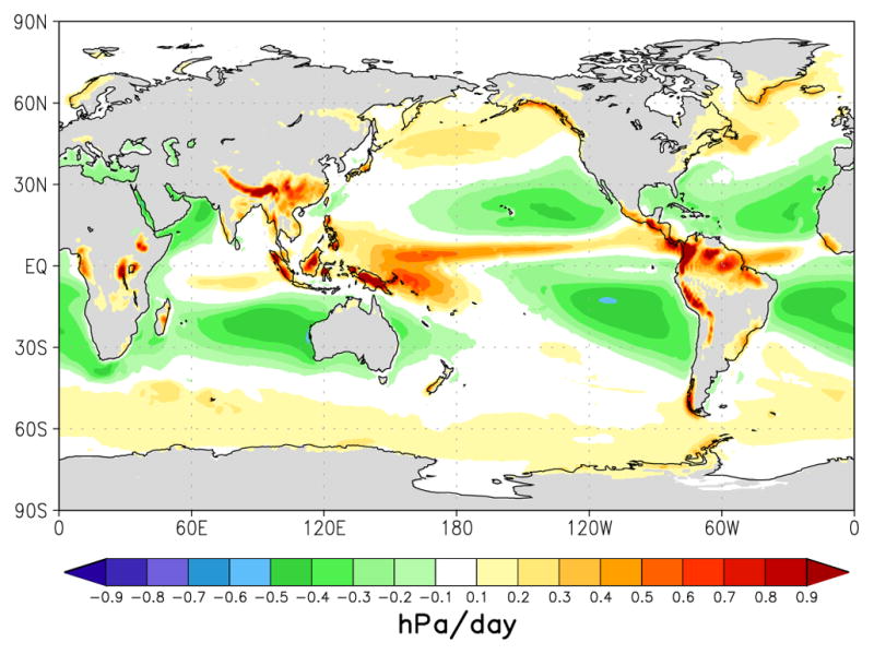
The effect of these transports can be seen in Fig. 6, which shows the change of precipitation minus evaporation that results from including mass sources and sinks. Although small (less than 1 kg m−2 day−1), these changes are statistically significant. They are largest in low latitudes and show increased water convergence in regions of heavy precipitation, such as the inter-tropical convergence zones, the South Pacific convergence zone, and the maritime continent. These changes are dominated by changes in precipitation, with evaporation changes being less than 0.2 kg m−2day−1.
Figure 6.

The change in the annual-mean climatology of surface precipitation minus evaporation as a result of adding sources of water mass to the model’s continuity equation. The heavy contour encloses regions of greater than 99% confidence that the two 30-year means differ, assuming individual annual means are independent. Units are kg m−2 day−1.
(b) ADAS evaluation
For an initial evaluation of the constraints on the model and analysis described in Section 2, we conducted three short experiments using variants of the assimilation system used in MERRA-2. All three used the same initial conditions, taken from an operational analysis for 15 February 2003, and were run through the end of March.
The first experiment (ADAS0) is meant to serve as a control; it is run in the traditional manner, with no constraint on dry-air mass variations or analysis increments of water.
The second experiment (ADAS1) includes the modifications to the model and analysis described in Sections 2a–c, which force the total mass of dry air to be invariant.
The third experiment (ADAS2) also guarantees the invariance of dry-air mass, but in addition, sets the global-mean analysis increment of water to zero, as described in Section 2d.
Figure 7 shows the evolution of the atmospheric mass in the three experiments. In the unconstrained experiment (ADAS0), there are large fluctuations in total mass that are unrelated to the water mass and result in large implied fluctuations in dry-air mass. In the two constrained experiments, total mass and water mass changes are forced to be identical, and the system accomplishes this by modifying the evolution of the total mass. The evolution of water mass is, in fact, quite insensitive to the treatment of the mass budget, showing a reasonable diurnal cycle and a smooth variation of sub-monthly anomalies in all experiments.
Figure 7.

Globally-integrated mass anomalies from the March mean for the three ADAS experiments (Top: ADAS0, Middle: ADAS1, Bottom: ADAS2). Shown are the total mass anomalies, as well as their decomposition into water (blue) and dry-air (orange) components.
To give a sense of how the change in the behavior of total mass comes about, we show in Fig. 8 a break-down of the total mass and water budgets. In ADAS0, the rate of change of total mass is simply the analysis tendency of surface pressure (red). The other three curves are the physical, analysis, and storage terms in the water budget. For ADAS1 and ADAS2, the water budget and the total mass budgets are identical. All quantities have been smoothed with a 24-hour running mean to eliminate a diurnal cycle that dominates the E − P and storage contributions.
Figure 8.

Evolution of the globally-integrated total water budget for the three ADAS experiments (Top: ADAS0, Middle: ADAS1, Bottom: ADAS2). Shown are the physical source term, E − P (blue), the analysis tendency (green), and the atmospheric water storage (black). For ADAS0, the analysis tendency of total atmospheric mass (red) is also plotted, with its values on the right axis. A 24-hour running mean has been applied to hourly values for all quantities.
We first note that even in ADAS0—without any of the constraints we are testing—the analysis increment of water is much smaller than it was in MERRA (Fig. 3), and the physical source term (E − P) and the water storage follow each other fairly closely. The tendency of total mass from the analysis of surface pressure, however, is much larger than any term in the water budget.
Compared to ADAS0, the monthly-mean analysis contribution to the water budget in ADAS1 is cut in half, with little change to other aspects of its evolution. The analysis contribution to total mass, on the other hand, is radically different. The smaller analysis tendency of water implies an even better balance between E − P and storage. In ADAS2, which ignores global-mean analysis contributions to both total mass or water mass, both budgets are, by construction, reduced to the same balance between E − P and storage.
It is noteworthy in Fig. 8 that the water storage contribution— the rate of change of the analyzed qw—is the most stable contribution to either budget. And that, as we increasingly constrain the budgets, the other terms, including E − P, adjust to its evolution. Figure 9 shows how the adjustment of E − P occurs. Practically all of the change in E − P comes from changes in precipitation. Not only is the level of evaporation the same in all experiments, most details of its evolution are also very similar. We conclude that the analysis of water vapour and the assimilation’s diagnosis of evaporation from analyzed winds, temperatures, and water vapor act as strong, and presumably reliable, anchors to both mass budgets.
Figure 9.

Evolution of globally-integrated precipitation and evaporation, for the three ADAS experiments. Units are kg m−2 day−1.
4. MERRA-2 results
The GMAO’s MERRA-2 reanalysis was run with a system very similar to the one used for the ADAS2 experiment discussed in Section 3. In particular, the MERRA-2 model and analysis separately conserve dry-air mass, and the global-mean analysis increments of both total mass and water mass are ignored. MERRA-2 is now complete through the end of 2014. Here we show results from the 30-year period from January 1985 through December 2014.
The top panel of Fig. 10 shows monthly anomalies of water mass, and the lower panel shows the breakdown of the globally-integrated water budget for MERRA-2. Note that with dry-air mass conservation, the evolution of water mass in MERRA-2 is identical to that of total mass. It consists of a nearly linear trend, disturbed by fairly large inter-annual events. This is similar to what we saw in the in the free-running AGCM experiment (Fig. 4) and in the other reanalyses, which for clarity, are reproduced here from Fig. 2. MERRA produced the largest trend, as the analysis took water from the system until 1998, when AMSU-A was introduced, and was either neutral or added water after that. MERRA-2 and ERA-Interim agree quite well — likely, mainly due to their similar treatment of the analysis variable as normalized RH —except for a short period in the early 90’s.
Figure 10.
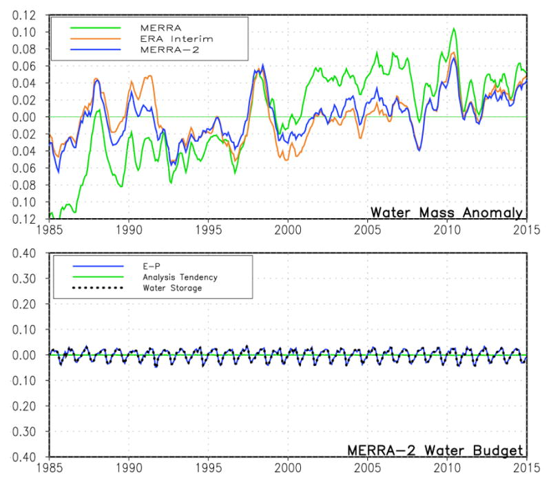
UPPER PANEL: Globally-integrated monthly mean water mass anomalies for the three reanalyses (Units are hPa). LOWER PANEL: The water budget in the MERRA-2 reanalysis, which can be compared with the other reanalyses plotted in Fig. 3 (Units are kg m−2 day−1).
For MERRA-2, the water budget (bottom panel of Fig. 10) consists of E − P and atmospheric water storage only, since the analysis increment is forced to be zero. This is in contrast to MERRA and ERA-Interim (Fig. 3), which, particularly MERRA, had large, spurious fluctuations in the analysis increments. These resulted in compensating fluctuations in E − P.
To compare with observations, we look at time series of column water vapor averaged over the ocean, for which we have long-term satellite observations from various microwave instruments. We will be comparing with the monthly product from Remote Sensing Systems Version-7 Release-0 (RSSV7; http://www.remss.com/measurements/atmosphericwater-vapor/tpw-1-deg-product), which are available from 1988 to present. Figure 11 shows the mean seasonal cycle and the evolution of monthly anomalies for the three reanalyses, for the free-running MERRA-2 model, and for the RSSV7 data. The MERRA and ERA-Interim mean values (inset) are lower than those for MERRA-2 and the observation, which not surprisingly, agree quite well, since RSSV7 SSM/I data were assimilated by MERRA-2. Nevertheless, the close agreement emphasizes how well these data constrain the column water vapor, particularly considering the large wet bias in the free-running model. Anomalies from the mean seasonal cycle show reasonable agreement between the five sources. MERRA-2, ERA-Interim, and the RSSV7 observations track each other very closely after the early 1990s. The trends for the 27-year period are 0.15 kg/m2/decade for MERRA2 and ERA-Interim, and 0.34 kg/m2/decade for RSSV7. The lower trends in MERRA-2 and ERA-Interim appear to be mostly due to a disagreement with the observations from 1988 to 1992.
Figure 11.
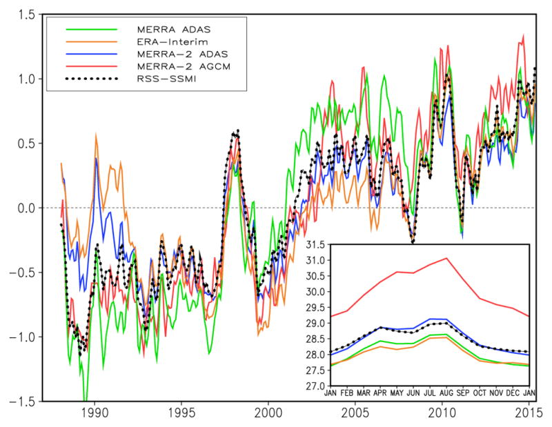
Climatological seasonal cycle (inset) and monthly anomalies of globally-integrated column water vapor over oceans. Units are kg m−2.
As a result of the constraints on the global hydrologic cycle, MERRA-2 produced a precipitation evolution that has to closely follow the relatively smooth evolution of evaporation. This is shown in Fig. 12, which again compares the three reanalyses. As noted earlier, we anticipated that other improvements in MERRA-2 would make it less sensitive to changes in the observing system, such as the jump in precipitation that occurred in MERRA with the introduction of AMSU-A in 1998. But even the smaller shifts in global precipitation, such as seen in ERA-Interim in 1992 and between 2002 and 2008, are absent from MERRA-2, whose total precipitation is now constrained by the evaporation.
Figure 12.

Globally-integrated evaporation (top panel) and precipitation (bottom panel) for MERRA, MERRA-2, and ERA-Interim reanalyses. Units are kg m−2 day−1.
Unlike the total water, the precipitation and evaporation in MERRA-2 show relatively little inter-annual variability, except for the long-term trends. Interestingly, precipitation and evaporation increase fairly dramatically early-on, flatten out after the turn of the century, and show a slight decrease in the last five years. This behavior is probably not compatible with surface temperature changes (see arguments surveyed by Allan et al. 2014) and must be due to changes in the observing system, particularly their impact on global evaporation.
In Fig. 12 we also see that the seasonal cycle of global precipitation and evaporation differ in the three reanalyses. In MERRA-2 seasonal changes in evaporation and precipitation are constrained to follow each other, and produced a fairly steady seasonal cycle, with an annual range slightly over 0.2 kg m−2 day−1. For the evaporation, this is also the case for the other two reanalyses, but their precipitation can be quite inconsistent. MERRA had almost no seasonal cycle of precipitation before 2000 and then shifted to one with large amplitude, while ERA-Interim has a somewhat irregular and weak precipitation cycle (weaker than its own evaporation) throughout the 30 years.
Finally, in Fig. 13, we consider the most direct effect of conserving dry-air mass by comparing the spatial distribution of the total mass budgets for MERRA and MERRA-2. The 30-year mean budget is separated into contributions from the physics, essentially E − P, from the dynamics, which is just the vertically-integrated mass convergence, and the mean analysis increment of surface pressure, which in MERRA-2 must produce an equivalent mass increment as the vertically-integrated analysis increment of total water. The physics contribution was, of course, not included in MERRA, so that panel does not appear. The dynamics and analysis contributions balance each other for MERRA, and for MERRA-2 the sum of the three panels is essentially zero.
Figure 13.

Comparison of the 30-year-mean total mass budgets of MERRA-2 and MERRA. Top Row: Surface pressure tendency due to the “physics” (as described in Section 2a), Middle Row: Surface pressure tendency due to dynamics, and Bottom Row: Surface pressure tendency due to the analysis.
We note first that both budgets are dominated by the analysis contribution, whose spatial distribution is similar in the two reanalyses. In both cases, the analysis moves mass from the oceans to the continents. The amplitude of this pattern, however, is considerably smaller for MERRA-2. In fact, it is small enough in low latitudes, that the vertically-integrated mass convergence from the reanalysis is clearly balancing E − P in the tropical convergence zones. The reduced magnitude of the analysis contribution in MERRA-2 is probably due to the analysis system drawing more weakly to surface pressure observations, rather than to the constraints on the mass budget that we have focused on here.
5. Summary
In this study we have considered the well-documented imbalances between globally-integrated precipitation and surface evaporation produced in the most recent reanalyses (Fig. 3). These imbalances are due to analysis adjustments to the specific humidity that are highly sensitive to changes in the observing system. In addition to water imbalances, reanalyses also produce changes in global-mean surface pressure that are not consistent with changes in global-mean water content. In fact, most of the variations in global-mean surface pressure come from spurious variations in the mass of dry air (Fig. 2).
We questioned whether we could usefully make simple modifications to the reanalysis system to conserve mass of dry air, so that variations of total water and total mass would agree. We also questioned whether we should retain the global-mean analysis increment of water, which drives imbalances in the water budgets and a large sensitivity of global-mean precipitation to the observing system.
We described in section 2 modifications made to all components (model, analysis, and IAU) of the data assimilation procedure such that globally-integrated dry-air mass is conserved, and precipitation and surface evaporation are in close balance. With this system we did three short assimilation experiments: with (1) no constraint, (2) conserving dry-air mass and (3) conserving dry-air mass and not allowing analysis increments of the total atmospheric water.
When we force the system to conserve dry-air mass, such that the analysis increments of water vapor and surface pressure must produce the same global-mean mass increment, we find that the system responds primarily by changing the surface pressure increments, with only modest changes to the water increments and E − P (Fig. 8). When, in addition, we ignore the global-mean analysis increment of water—forcing E − P to exactly balance the analyzed changes in total water—the system responds by primarily changing E − P. In both cases the system accepts the mass estimate from the water analysis, and in the latter case, when it changes E − P, the change is mostly in the precipitation (Fig. 9).
Having found no obvious deleterious impact of constraining either the dry-air mass variability or the analysis increment of water in preliminary experiments, we applied both constraints to the MERRA-2 reanalysis. Since the MERRA and MERRA-2 systems differ in many other ways, it is hard to identify specific effects of using the constraints. Certainly abrupt changes in the global hydrologic cycle—such as we saw in E − P in earlier reanalyses (Fig. 3)—are trivially absent in MERRA-2 (Fig. 10, lower panel); but we cannot say, from the very preliminary analysis we have been able to perform, how their absence may have affected other aspects of the reanalysis.
As in the preliminary experiments, forcing the global E − P to be small in MERRA-2 produces a better behaved precipitation, with a regular seasonal cycle and no sudden shifts (Fig. 12). But observing system sensitivity still produces surprisingly large trends, such as the systematic increase in precipitation and evaporation from 1985 to 2000 and their decline from 2010 to 2015. Understanding these will be the next step in developing a reanalysis that properly captures the hydrologic cycle of a changing climate.
Acknowledgments
The authors thank their colleagues at NASA’s Global Modeling and Assimilation Office for discussions in group meetings throughout the development of this work, in particular: Stephen Bloom, Ronald Gelaro, William McCarty, Andrea Molod, and the entire MERRA-2 team. We also thank Atanas Trayanov for help dealing with software issues. Finally, we are indebted to two anonymous reviewers, whose very helpful comments led to major revisions of the manuscript. Experiments were carried out using the Linux cluster at the NASA Center for Climate Simulation.
Appendix: Treatment of Non-Water Constituents
In Section 2, we discussed modifications made to the total air mass and to the water constituents, which are now part of the total mass balance. The system, however, carries a number of other constituents or tracers not involved in the total mass balance whose update must also be addressed. The model handles these trivially by using (3b). If there are analysis increments of total mass, however, we must make some assumption regarding the constituent concentration of the added or removed mass. This is true whether we hold the dry-air mass invariant or not.
Obviously, the water part of the mass increment cannot affect the constituent’s mass (although it will affect its qk), we must make an assumption about the composition of the dry-air part. We consider two assumptions: (1) that the dry air added or removed has the same composition as the mean dry air in the grid box, or (2) that we add or remove dry air that has none of the constituent in question.
The first assumption implies that a constituent’s fractional mass with respect to dry air, , is unaltered:
| (14) |
Here, the superscript f refers to the desired “final” value after all updates, and b to the value “before” the analysis update of mass is applied. In the case that the constituent is itself explicitly analyzed, its increment is added before the atmospheric mass is updated, and so is already included in the “before” values. With this assumption, a constituent with a uniform mixing ratio—which would remain uniform in the presence of advective or mixing processes—will also remain uniform when dry air is subject to analysis increments. It does, however, alter the local value of constituent fractional mass qk, since from (14)
| (15) |
We can compare this result to the second approach, in which the constituent’s layer mass is always conserved and we obtain the final qk from
| (16) |
and the final dry-air mass fraction from
| (17) |
In this case, the constituent’s dry-air mass fraction is preserved only when there is no analysis adjustment to the mass of dry air in the layer. This is very undesirable, since local analysis increments of surface pressure will result mostly in increments to the dry-air mass. We have therefore adopted the first approach for non-water constituents, but with an additional constraint to conserve the globally-integrated constituent mass through a “fixer” similar to those discussed in Section 2.
References
- Allan Richard P, Liu Chunlei, Zahn Matthias, Lavers David A, Koukouvagias Evgenios, Bodas-Salcedo Alejandro. Physically Consistent Responses of the Global Atmospheric Hydrological Cycle in Models and Observations. Surveys in Geophysics. 2014;35:533–552. [Google Scholar]
- Berrisford P, Kallberg P, Kobayashi S, Dee D, Uppala S, Simmons AJ, Poli P, Sato H. Atmospheric conservation properites in ERA-Interim. Quart J Roy Meteor Soc. 2011;137:1381–1399. [Google Scholar]
- Bloom S, Takacs L, DaSilva A, Ledvina D. Data assimilation using incremental analysis updates. Mon Wea Rev. 1996;124:1256–1271. [Google Scholar]
- Dee DP, da Silva AM. The choice of variable for atmospheric moisture analysis. Mon Wea Rev. 2003;131:155–171. [Google Scholar]
- Dee DP, et al. The ERA-Interim reanalysis: Configuration and performance of the data assimilation system. Quart J Roy Meteor Soc. 2011;137:553–597. doi: 10.1002/qj.828. [DOI] [Google Scholar]
- Derber JC, Rosati A. A global oceanic data assimilation system. J Phys Oceanography. 1989;19:1333–1347. [Google Scholar]
- El Akkraoui A, Tremolet Y, Todling R. Preconditioning of variational data assimilation and the use of a bi-conjugate gradient method. Quart J Roy Meteor Soc. 2013;139:731–741. [Google Scholar]
- Held IM, Soden BJ. Robust Responses of the Hydrological Cycle to Global Warming. J Climate. 2006;19:5686–5699. [Google Scholar]
- Holm EV. Proc Workshop on Humidity Analysis. Reading, U.K: ECMWF/GEWEX; 2003. Revision of the ECMWF humidity analysis: Construction of a Gaussian control variable; pp. 1–6. [Available online from http://old.ecmwf.int/publications/library/ecpublications/pdf/workshop/2002/Humidity/holm.pdf] [Google Scholar]
- Kleist DT, Parrish DF, Derber JC, Treadon R, Wu W-S, Lord S. Introduction of the GSI into the NCEPs Global Data Assimilation System. Wea Forecasting. 2009;24:1691–1705. [Google Scholar]
- Lin SJ. A Vertically Lagrangian Finite-Volume Dynamical Core for Global Models. Mon Wea Rev. 2004;132:2293–2307. [Google Scholar]
- Massart S, Pajot B, Piacentini A, Pannekoucke O. On the merits of using 3D-FGAT assimilation scheme with an outer loop for atmospheric situations governed by transport. Mon Wea Rev. 2010;138:4509–4522. [Google Scholar]
- Rienecker MM, Suarez MJ, Gelaro R, Todling R, Bacmeister J, Liu E, Bosilovich MG, Schubert SD, Takacs L, Kim G-K, Bloom S, Chen J, Collins D, Conaty A, da Silva A, et al. MERRA: NASA’s Modern-Era Retrospective Analysis for Research and Applications. J Climate. 2011;24:3624–3648. doi: 10.1175/JCLI-D-11-00015.1. [DOI] [PMC free article] [PubMed] [Google Scholar]
- Robertson FR, Bosilovich MG, Chen J, Miller TL. The Effect of Satellite Observing System Changes on MERRAWater and Energy Fluxes. J Climate. 2011;24:51975217. [Google Scholar]
- Trenberth KE, Smith L. The Mass of the Atmosphere: A Constraint on Global Analysis. J Climate. 2005;18:864–875. [Google Scholar]
- Trenberth KE, Fasullo JT, Mackaro J. Atmospheric Moisture Transports from Ocean to Land and Enery Flows in Reanalysis. J Climate. 2011;24:4907–4924. [Google Scholar]
- Trenberth KE, Fasullo JT. Regional energy and water cycles: transports from ocean to land. J Climate. 2013;26:78377851. [Google Scholar]
- Uppala SM, et al. The ERA-40 re-analysis. QJR Meteorol Soc. 2005;131:2961–3012. doi: 10.1256/qj.04.176. [DOI] [Google Scholar]
- Wu WS, Purser RJ, Parrish DF. Three-dimensional variational analysis with spacially inhomogeneous covariances. Mon Wea Rev. 2002;130:2905–2916. [Google Scholar]