Online Conditional Outlier Detection in Nonstationary Time Series

Abstract

The objective of this work is to develop methods for detecting outliers in time series data. Such methods can become the key component of various monitoring and alerting systems, where an outlier may be equal to some adverse condition that needs human attention. However, real-world time series are often affected by various sources of variability present in the environment that may influence the quality of detection; they may (1) explain some of the changes in the signal that would otherwise lead to false positive detections, as well as, (2) reduce the sensitivity of the detection algorithm leading to increase in false negatives. To alleviate these problems, we propose a new two-layer outlier detection approach that first tries to model and account for the nonstationarity and periodic variation in the time series, and then tries to use other observable variables in the environment to explain any additional signal variation. Our experiments on several data sets in different domains show that our method provides more accurate modeling of the time series, and that it is able to significantly improve outlier detection performance.

Introduction

Outlier, or anomaly, detection has been widely studied in the data mining and machine learning communities (Chandola, Banerjee, and Kumar 2009). It aims to identify out-of-ordinary data instances, i.e., instances that are very different from the rest of the data. Most previous research work deals with outlier detection for independent and identically distributed (iid) data. Our focus in this work, however, is on outlier detection methods for time series data, where data instances may be linked by complex temporal dependencies. Our goal is to develop outlier detection methods analyzing time series in real time and being able to identify, as quickly as possible, aberrant time-series readings. Such methods are extremely important for the development of various monitoring and alerting applications that help humans to screen behaviors of both natural, as well as, man-made systems.

Real-world time series data may exhibit complex temporal behaviors due to various sources of variability that may influence their expression. One possible source of variability is a periodic or seasonal variation of the signal. For example, monitoring of various web-based human activities may vary depending on what day of the week and what hour of the day the signal is associated with. Similarly, monitoring of the sea level is affected by moon gravity and low-and-high-tide variation. Other sources of variations may be due to other effects of the environment. Briefly, any variable representing some aspect of the environment may influence the observed time series, being reflected in its readings. If this variable is observed but ignored, the readings alone may look aberrant. In general, additional environmental variables, whenever they are observed and considered, may explain the time series and its variation. As an example, consider the time series of web-based human activities discussed above, and assume the day we collect the current reading for is a holiday. In that case, the readings are likely to be different from the regular days of the week, and changes in the readings may be explained by the information about holidays. Similarly, the readings of the sea level may be affected by the weather pattern, for example, the presence of the storm in the area.

A variety of sources of variability and their combined effects make the problem of outlier detection for time series a very challenging problem, especially when many environmental variables are considered, and the time series we work with and analyze are relatively short and do not provide many examples of the behaviors for the different sources of variability. For example, even if we have one year worth of data for the time series, the number of holidays in one year remains relatively low. In this work, we tackle the problem by developing a new two-layer outlier detection method for nonstationary time series. In the first layer, our procedure tackles periodic variations and other nonstationarity. By accounting for these variations, it calculates local deviation scores that measure the deviation of the most recent time-series readings. However, some of the outlier-looking signal may still be explained by other environmental variables. This is the focus of the second layer of the procedure, that attempts to correlate the local deviation scores with the context variables and hence explain it.

To implement the first layer we use a nonparametric method, Seasonal-Trend decomposition, or STL (Cleveland et al. 1990). STL decomposes the time series into three components: seasonal, trend, and remainder. As the seasonal and trend are smoothed, outliers tend to aggregate in the remainder. To implement the second layer, we use Bayesian linear regression, so we can add uncertainty to the model to accommodate the scarcity of examples for different sources of variability.

We test our approach and show its benefits on data sets in three different domains: time series of daily bike rental counts, time series of daily alert rule firings generated by the monitoring and alerting components embedded in a clinical decision support system, and time series of vehicular traffic volumes generated by sensors placed on major highways.

Related Work

Early work in outlier detection in time series comes from the statistical literature. In (Fox 1972), the authors define two types of outliers, additive outliers (AO) and innovational outliers (IO). They consider the autoregressive (AR) model and develop likelihood ratio tests for detecting outliers. In addition to AO and IO, (Tsay 1988) introduce and study two other types of outliers, level shift (LS) and variance change (VC). The model is extended to autoregressive moving-average (ARMA). They study the effects of different outliers on the time series and propose different tests to detect them. Their outlier detection procedure is iterative and cycles among parameter estimation and outlier detection/removal. (Chen and Liu 1993) propose to jointly estimate multiple outlier effects and model parameters, instead of removing outliers one by one as in the previous work. However, their procedure is still iterative.

All of the above work differs from ours in at least two aspects. First, their methods are retrospective, i.e., they assume the whole time series is available, and they look back to find all outliers in the past. In contrast, our work focuses on online detection, where we want to detect outliers in the newly observed data as soon as they arrive. Second, the above methods assume the time series follow the ARMA model and raise an alarm if a data point significantly deviates from the model. However, ARMA assumes the time series is second-order stationary. But in reality, this assumption usually does not hold, because (a) a time series can have seasonality; (b) a time series can have a trend. We note that (a) and (b) can be addressed by adding (seasonal) differencing to the model, resulting in the seasonal autoregressive integrated moving average (SARIMA) model (Box et al. 2015; Shumway and Stoffer 2010). However, normal points differenced with outliers become “false outliers” and result in false alarms. Also, all these models predict future data from past data. When there is an outlier in the past data, the future data, though normal, may be labeled as outliers due to deviation from the biased prediction. Therefore, these models are not suitable for online outlier detection in nonstationary time series.

More recently, (Yamanishi and Takeuchi 2002) develop an online algorithm for nonstationary time series. The authors assume the time series follow the autoregressive (AR) model and introduce a sequential discounting algorithm to estimate its parameters and to make inference. However, as they assume AR, which is a subset of ARMA, their method suffers the same problems as the above methods.

(Laptev, Amizadeh, and Flint 2015) propose an outlier detection framework for time series data that lets one to exclude outliers that may be explained by context variables. This is done by defining rules on these variables. For example, one may define a rule checking whether a day is a holiday and exclude all these days from consideration. One limitation of this approach is that it prevents us from detecting outliers that differ from typical holiday patterns. Our approach does not have this limitation, since it statistically models and detects outliers conditioned on the context variables. Another limitation is that building these rules requires human knowledge. In contrast, our method learns a statistical model automatically from available data, so human knowledge is not necessary. It gives us the flexibility to add all available variables that might be useful for detecting outliers, and let the data to decide which are more relevant than the others.

Finally, (Hauskrecht et al. 2013) develop methods for conditional outlier detection on clinical time series mined from EHR. The approach is built to detect outliers on subset of discrete valued variables given the rest of the variables and relies on template featurization that converts time series to fixed feature vectors. It also assumes the feature vectors are iid. Our work focuses on counts and real-valued time series, and online detection methods.

Preliminaries: STL

We start by introducing the Seasonal-Trend decomposition, or STL (Cleveland et al. 1990), that is used as a building block for our first-layer model. STL is a nonparametric decomposition algorithm that applies locally weighted regression, or LOESS (Cleveland and Cleveland 1979; Cleveland and Devlin 1988). Given a set of points {(x_i, y_i) : i = 1,…, n}, LOESS fits a smoothed curve y = g(x). For any x, to compute g(x), it fits a d-degree polynomial to {(x_i, y_i)} weighted by $v_i\left(x\right)=W\left(\frac{|x_i-x|}{{\mathrm{\lambda }}_q\left(x\right)}\right)$, where W (u) = (1 − u³)³, if u ∈ [0, 1], and 0 otherwise. λ_q(x) is the distance between x and its q-th nearest neighbor in {x_i}. If q > n, it is ${\mathrm{\lambda }}_n\left(x\right)\frac{q}{n}$.

The main steps of STL are as follows. To separate out seasonal signal, STL fits a curve to each subseries that consists of the points in the same phase of the cycles in the time series. After removing the seasonal signal, it fits another curve to all the points consecutively to get the trend. The residuals after further removing the trend are called remainders.

It is worth noting that STL is a robust algorithm. It deals with outliers by down-weighting them and iterating the procedure. The bisquare weight function, B(u) = (1 − u²)², if u ∈ [0, 1], and 0 otherwise, is used for this purpose, where u is the normalized remainder for each point.

Method

In this section, we introduce our method. Let the time series be y = {y_t ∈ ℝ : t = 1, 2, …} with context variables x = {x_t ∈ ℝ^p : t = 1, 2 …}. Our goal is to compute an outlier score v_t ∈ ℝ at each t based on the data available at t. Our method consists of two layers. In the first layer, we remove nonstationarity and temporal dependencies from the data and derive the local deviation scores. In the second layer, we model the local deviation scores conditioned on the context variables by Bayesian linear regression. We adopt Bayesian inference because it supports more robust online learning by allowing us to add uncertainty to the model through priors. This is important, because typically context variable observations for learning the second layer model are scarce at the beginning (e.g. the number of observed holidays is small). Adding uncertainty can reduce false alarms caused by high variance in the estimated parameters.

First-Layer Model

The first-layer model takes the input time series, y, and outputs a sequence of local deviation scores, z. Since the time series are usually nonstationary and may even have structural changes (nonstationarity other than seasonality and trend), we use a sliding window to restrict the time span considered, and assume that the time series in an appropriate-sized window does not have structural changes. Let n_(p) be the period of y. The window size u cannot be too small compared to n_(p) because STL needs enough cycles of data for smoothing. But also it cannot be too large due to nonstationarity. We found 5n_(p) is good to be used as a default value.

At time t, for the local time series of length u in the window, y_u(t) = {y_(t−u+1), y_(t−u+2),…, y_t}, STL is applied to decompose it into trend, seasonal, and remainder. On the remainder, r(y_u(t)), we calculate the deviation, z_t, of the last point, r(y_t), from the population

$$z_t=\frac{r\left(y_t\right)-{\widehat{\mu }}_t}{{\widehat{\sigma }}_t},$$ (1)

where ${\widehat{\mu }}_t$ and ${\widehat{\sigma }}_t$ are estimators of the population mean and standard deviation. We use the common choices: the sample mean and the sample standard deviation.

By sliding the window as new data arrive, we get a sequence of the local deviation scores, z, as the output of the first-layer model.

Second-Layer Model

The second-layer model takes the output of the first-layer model, z, and a time series of context variables, x, as input, and outputs a sequence of final outlier scores, v. We adopt a Bayesian approach to model z_t given x_t. Specifically, we assume the following linear model

$$z_t|w,\beta ,x_t~N\left(x_t^{T}w,{\beta }^{-1}\right).$$

That is, given w, β and x_t, z_t follows a normal distribution. For the prior distribution of (w, β), we use the conjugate prior, which is a normal-Gamma distribution

$$w,\beta ~N(w|m_0,{\beta }^{-1}{S}_0)\mathit{Gam}(\beta |a_0,b_0),$$

where we use the following parameterization for the probability density function (pdf) of the Gamma distribution

$$f\left(\beta |a,b\right)=\frac{b^a}{\mathrm{\Gamma }\left(a\right)}{\beta }^{a-1}{e}^{-b\beta }.$$

Let D_t = {(z₁, x₁), (z₂, x₂), …, (z_t, x_t) denote the data we observe so far at time t. When we observe a new sample (z_t+1, x_t+1), the posterior distribution for (w, β) is again normal-Gamma with updated parameters

$$\begin{array}{l}w,\beta |D_t,z_{t+1},x_{t+1}\\ ~N\left(w|m_{t+1},{\beta }^{-1}{S}_{t+1}\right)\mathit{Gam}\left(\beta |a_{t+1},b_{t+1}\right),\end{array}$$

where

$$\begin{array}{l}{S}_{t+1}^{-1}=S_t^{-1}+x_{t+1}{x}_{t+1}^T,\\ m_{t+1}=S_{t+1}\left(S_t^{-1}{m}_t+z_{t+1}+x_{t+1}\right),a_{t+1}=a_t+\frac{1}{2},\\ b_{t+1}=b_t+\frac{1}{2}\left(z_{t+1}^2-m_{t+1}^T{S}_{t+1}^{-1}{m}_{t+1}+m_t^T{S}_t^{-1}{m}_t\right).\end{array}$$ (2)

The predictive distribution for z, given D_t and the corresponding context variable x, is a Student’s t-distribution with location and scale

$$z|D_t,x~St\left(z|\mu ,{\sigma }^2,\nu \right)$$

where the pdf of the distribution is

$$f\left(z|\mu ,{\sigma }^2,\nu \right)=\frac{\mathrm{\Gamma }\left(\frac{\nu +1}{2}\right)}{\mathrm{\Gamma }\left(\frac{\nu }{2}\right)\sqrt{\pi \nu {\sigma }^2}}{\left(1+\frac{1}{\nu }\frac{{\left(z-\mu \right)}^2}{{\sigma }^2}\right)}^{-\frac{\nu +1}{2}},$$

and

$$\nu =2a_t,\mu =x^T{m}_t,{\sigma }^2=\frac{b_t}{a_t}\left(1+x^T{S}_{t}x\right).$$ (3)

We define the outlier score for z_t+1, given D_t and x_t+1, as

$$v_{t+1}=1-p_{t+1}=1-P\left(|T_{\nu }|>\frac{|z_{t+1}-\mu |}{\sigma }\right),$$ (4)

where T_ν follows the standard t-distribution with ν degree(s) of freedom, and p_t+1 is the probability of z_t+1 taking a more extreme value than the current value.

In summary, for t = 0, 1, …, given (z_t+1, x_t+1), we compute the outlier score as in (3) and (4). Then, we update the distribution of the parameters as in (2).

Experimental Evaluation

We evaluate our method on time series data from three different domains.

Bike data consists of the time series (of length 733) that record the daily bike trip counts taken in San Francisco Bay Area through the bike share system from August 2013 to August 2015¹. Additional context variables available for the count data are holiday indicators and weather data. The weather data include precipitation, cloud cover, wind direction, mean temperature, mean dew point, mean humidity, mean sea level pressure, mean visibility, and mean wind speed. For temperature, we perform a preprocessing that transforms the value into the absolute value of the local deviation (similar to (1) with absolute value), because we expect both very high and very low temperatures to have an impact the number of bike trips. Outliers detected in such a time series may reflect various unaccounted events influencing the number of bike rentals, including unexpected closures due to malfunctions of the rental system.

CDS data consists of daily rule firing counts of a clinical decision support (CDS) system in a large teaching hospital (Wright et al. 2016). The rules in the CDS are used to either alert on some adverse conditions or recommend certain actions (such as vaccinations). The data include time series for 111 such rules, and each time series is of length 1187. Additional context variables collected are holiday indicators and the number of electronic health records (EHR) opened. Both are believed to influence the rule firings. Holidays may reduce the number of visits, and the number of EHR opened may give a rough estimate of the number of patients potentially screened by the rules during that day. Outliers may reflect the different events influencing the rules such as the beginning of the flu season, or CDS system malfunctions that may lead to rule silencing or aberrant rule firings.

Traffic data consists of time series of vehicular traffic volume measurements collected by sensors placed on major highways in Pittsburgh area (Šingliar and Hauskrecht 2010). The time series we use here are sampled at a fixed time across days for a year. We use data from two such sensors. The context variable available for these data is holiday indicator. Outliers in the time series may indicate traffic accidents, road repairs, severe weather patterns, or events such as concerts that lead to the surge in the traffic.

Experiment Setup

Since there are no outliers marked for our data, we test the performance of the detection methods on simulated outliers that correspond to randomly introduced changes in the original signal. More specifically, outliers are injected into the time series by randomly sampling a small percentage p of points and changing the value by a specified size δ as y_i = y_i · δ for each point y_i. The values are rounded to the closest integers, so they are still counts. We use multiplicative change instead of additive, because the data show heteroscedasticity (the variance increases as the mean increases). We set p = {0.01, 0.05, 0.1} and δ = {2=1, 3=2, 6=5, 5=6, 2=3, 1=2} respectively to see the influence of different settings on the performance. We consider the injected outliers as the ground-truth outliers when evaluating the performance.

Methods

We compare the following methods:

• RND - detects outliers randomly.

• SARI - ARIMA(1, 1, 0) × (1, 1, 0)₇, SARIMA (Box et al. 2015) with a weekly period, (seasonal) differencing, and (seasonal) order 1 autoregressive term.

• SIMA - ARIMA(0, 1, 1) × (0, 1, 1)₇, SARIMA with a weekly period, (seasonal) differencing, and (seasonal) order 1 moving-average term.

• SARIMA - ARIMA(1, 1, 1) × (1, 1, 1)₇, SARIMA combining the above two.

• ND - our first-layer model, using the absolute value of the output as outlier scores.

• TL1 - our two-layer model using holiday information as a context variable.

• TL2 - our two-layer model using holiday and additional information (if available) as context variables.

For all the ARIMA based methods we also use a sliding window. We estimate the parameters from the past points and make a prediction for the latest point. The outlier scores are derived similarly as in (4).

We use R for all the experiments. All methods compared use a sliding window of size 35 (5n_(p)). The hyperparameters for the two-layer method are m₀ = 0, S₀ = I, a₀ = 1, and b₀ = 100, where I is the identity matrix. They are not tuned, but we intentionally set the prior variance to make the model uncertain when the data are still scarce, so it does not raise many false alarms at the beginning. We add a bias term for the regression. For STL, we set the seasonal smoothing window size, n_(s) = 7, which is the smallest reasonable value according to (Cleveland et al. 1990), and n_(p) = 7, for the weekly periodicity, and use recommended values for the other parameters.

Because our data are counts and show heteroscedasticity, the square-root transformation, $\sqrt{x+0.5}$, is applied to stabilize the variance for all methods (Bartlett 1947).

Evaluation

We use precision-alert-rate (PAR) curves to evaluate the methods (Hauskrecht et al. 2016). Outlier detection methods are usually applied in monitoring and alerting systems, where the alert rate needs to be controlled by setting a threshold for the outlier score. The precision for a given alert rate is the most important factor in evaluating the performance, because whether it is high or low decides whether the system is useful or annoying, even harmful (Hauskrecht et al. 2016). If the alert rate and the precision are not well-controlled, it may lead to so-called alert fatigue (Lee et al. 2010; Embi and Leonard 2012), that is users stop responding to the alerts due to their ineffectiveness. Since the probability of getting an outlier is assumed to be low by definition, alert rates cannot be set to be high in reality.

We do not use precision-recall (PR) curves to evaluate the methods, because in reality, it is usually very hard to get all the outliers without causing alert fatigue. People instead control the alert rate while maintaining good precision. However, for completeness, we did evaluation with PR curves (not included due to space limit), and the results show the advantages of our method as well.

Results

Figure 1 shows the PAR curves for Bike data with different outlier rates, p, and different outlier sizes (folds of changes), δ leading to 18 data sets. The results are organized in a grid with different folds of changes in rows, and different outlier rates in columns. The maximum alert rate is kept at 0.1 (10% of data). We show the precision at different alert rates. The results show that it is easier to detect stronger outliers (corresponding to a larger fold of change), which is expected, since they are more likely to rise above the natural noise in the data. If the outlier signal is very weak, it may fall into the natural noise level, which is reflected by the PAR curves approaching RND. Also, as expected, the precision generally is higher, when more outliers are injected in the data.

Figure 1.

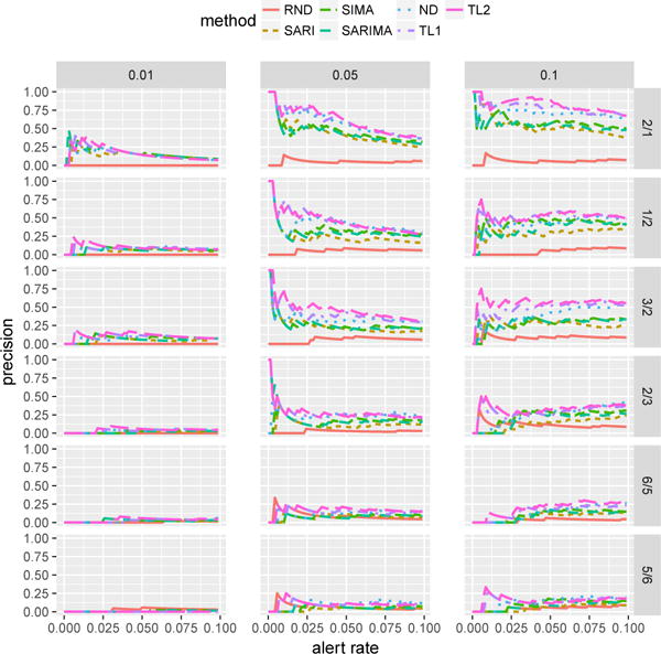
PAR curves for Bike data. Each column has a different rate for injection of outliers, indicated by the labels at the top. Each row has a different size (fold of change) for outliers, indicated by the labels on the right.

Comparing the detection methods tested, we see the two versions of our two-layer method outperform other methods with the margin increasing for stronger and more frequent outliers. To make the comparison in different settings easier, we calculate the areas under the PAR curves (AUC-PAR). To make them comparable for different outlier rates, we normalize the alert rate relative to the outlier rates. That is, we calculate the precisions at alert rates corresponding to α times the outlier rate p, where α ∈ [0, 1], and normalize the AUC to be in [0, 1]. Table 1 shows the AUC-PAR for Bike data. Similar to the results in Figure 1, our two-layer methods are the best performing methods across a wide range of outlier sizes (folds) and rates.

Table 1.

AUC-PAR for Bike data.

rate	fold	RND	SARI	SIMA	SARIMA	ND	TL1	TL2
0.01	2/1	0.00	0.09	0.16	0.24	0.14	0.19	0.16
0.01	1/2	0.00	0.00	0.00	0.00	0.00	0.05	0.09
0.01	3/2	0.00	0.00	0.00	0.00	0.00	0.05	0.05
0.01	2/3	0.00	0.00	0.00	0.00	0.00	0.00	0.00
0.01	6/5	0.00	0.00	0.00	0.00	0.00	0.00	0.00
0.01	5/6	0.00	0.00	0.00	0.00	0.00	0.00	0.00
0.05	2/1	0.05	0.56	0.56	0.55	0.71	0.75	0.77
0.05	1/2	0.04	0.31	0.38	0.35	0.48	0.58	0.57
0.05	3/2	0.03	0.33	0.30	0.31	0.38	0.47	0.55
0.05	2/3	0.02	0.13	0.16	0.23	0.24	0.31	0.32
0.05	6/5	0.12	0.07	0.06	0.06	0.10	0.15	0.17
0.05	5/6	0.09	0.02	0.04	0.05	0.08	0.10	0.11
0.1	2/1	0.06	0.54	0.58	0.55	0.72	0.78	0.82
0.1	1/2	0.04	0.29	0.42	0.36	0.44	0.51	0.52
0.1	3/2	0.09	0.27	0.27	0.29	0.38	0.49	0.56
0.1	2/3	0.11	0.12	0.22	0.19	0.25	0.29	0.32
0.1	6/5	0.03	0.08	0.10	0.09	0.13	0.16	0.20
0.1	5/6	0.05	0.05	0.10	0.08	0.14	0.14	0.15

We have performed the same experiments on CDS and Traffic data. Due to the space limit, we only show AUC-PAR. The results are compiled in Table 2 and 3 respectively. We note that for these two data sets we have multiple time series, so we report the averaged results. That is, given an alert rate, we average the precision over all time series. Once again the results show that our two-layer method outperforms the baselines.

Table 2.

AUC-PAR for CDS data.

rate	fold	RND	SARI	SIMA	SARIMA	ND	TL1	TL2
0.01	2/1	0.00	0.06	0.05	0.05	0.03	0.07	0.12
0.01	1/2	0.01	0.02	0.02	0.02	0.03	0.03	0.05
0.01	3/2	0.00	0.02	0.02	0.02	0.02	0.02	0.03
0.01	2/3	0.00	0.02	0.02	0.02	0.02	0.02	0.02
0.01	6/5	0.01	0.01	0.01	0.01	0.02	0.02	0.01
0.01	5/6	0.01	0.01	0.01	0.01	0.02	0.02	0.01
0.05	2/1	0.05	0.22	0.22	0.22	0.25	0.30	0.35
0.05	1/2	0.05	0.10	0.11	0.11	0.16	0.17	0.22
0.05	3/2	0.05	0.11	0.11	0.11	0.14	0.14	0.19
0.05	2/3	0.05	0.07	0.08	0.08	0.11	0.10	0.13
0.05	6/5	0.05	0.07	0.07	0.07	0.08	0.07	0.08
0.05	5/6	0.05	0.06	0.06	0.06	0.08	0.07	0.07
0.1	2/1	0.10	0.32	0.37	0.35	0.43	0.47	0.53
0.1	1/2	0.10	0.18	0.22	0.21	0.30	0.31	0.36
0.1	3/2	0.10	0.20	0.22	0.21	0.28	0.28	0.34
0.1	2/3	0.10	0.13	0.15	0.14	0.22	0.21	0.24
0.1	6/5	0.10	0.14	0.14	0.14	0.17	0.16	0.17
0.1	5/6	0.09	0.11	0.12	0.11	0.15	0.14	0.15

Table 3.

AUC-PAR for Traffic data.

rate	fold	RND	SARI	SIMA	SARIMA	ND	TL1
0.01	2/1	0.00	0.50	0.50	0.58	0.50	0.64
0.01	1/2	0.00	0.42	0.39	0.39	0.14	0.58
0.01	3/2	0.00	0.00	0.11	0.11	0.11	0.47
0.01	2/3	0.00	0.03	0.14	0.11	0.11	0.00
0.01	6/5	0.00	0.00	0.00	0.00	0.00	0.00
0.01	5/6	0.00	0.00	0.00	0.00	0.00	0.00
0.05	2/1	0.18	0.61	0.74	0.69	0.67	0.85
0.05	1/2	0.04	0.29	0.36	0.35	0.39	0.55
0.05	3/2	0.00	0.29	0.43	0.40	0.41	0.53
0.05	2/3	0.21	0.14	0.26	0.22	0.19	0.28
0.05	6/5	0.00	0.06	0.03	0.02	0.05	0.08
0.05	5/6	0.07	0.04	0.03	0.06	0.01	0.03
0.1	2/1	0.12	0.61	0.74	0.68	0.74	0.86
0.1	1/2	0.05	0.28	0.47	0.43	0.54	0.61
0.1	3/2	0.11	0.38	0.52	0.45	0.51	0.63
0.1	2/3	0.07	0.13	0.30	0.26	0.27	0.30
0.1	6/5	0.12	0.19	0.18	0.19	0.18	0.21
0.1	5/6	0.10	0.06	0.10	0.10	0.07	0.07

By comparing the results across different data sets, we notice that the quality of the detection may vary widely. This is due to the properties of the original time series. For example, while Bike data is relatively clean, Traffic and especially CDS data have much more noise and irregularities, that are detected as outliers. Hence the precision calculated based on injected outliers gets smaller.

Comparing ND with ARIMA based methods, we notice that ND performs either close to or better than the others in almost all the experiments. We think the main reason is that ND accounts for seasonality without differencing, so it does not “pollute” normal points like ARIMA based methods.

Comparing TL1 with ND and ARIMA based methods, we see an advantage in most cases. This confirms our assumption that whether the day is a holiday has a significant influence on the value observed on that day. TL1 makes use of that information to explain some of the “outliers” in the data. This can largely reduce the number of false alarms and therefore increase the precision.

Comparing TL2 with TL1, TL2 dominates TL1 in almost all cases. This proves the usefulness of additional information (EHR counts for CDS data and weather for Bike data), and demonstrates the flexibility of our method. Whenever there is new potentially useful information, we can add it as new context variable(s) to improve the performance. In reality, it is hard to tell beforehand which context variables will be helpful for detecting outliers. For our method, we can just add all the variables that might be helpful and have the model learn which are. This, we think, is a big advantage over a rule-based model, which needs expert knowledge and/or trial-and-error to find out which variables are useful and to define correct rules to filter out false alarms.

Conclusion

We have developed a new two-layer method for online outlier detection in nonstationary time series. The first layer removes non-stationarity and temporal dependencies and computes the local deviation scores. The second layer makes use of the context variables, which may explain some “outliers” in the data, through Bayesian linear regression on the first-layer output. We tested the method using data sets from three different domains. Compared with traditional methods, our method can handle nonstationary time series and use context variables to filter out explicable “outliers”, resulting in reduced false alarms and increased precision at reasonable alerting rates, which is of crucial importance for building monitoring and alerting systems.

References

- Bartlett MS. The Use of Transformations. Biometrics. 1947;3(1):39–52. [PubMed] [Google Scholar]
- Box GE, Jenkins GM, Reinsel GC, Ljung GM. Time Series Analysis: Forecasting and Control. John Wiley & Sons; 2015. [Google Scholar]
- Chandola V, Banerjee A, Kumar V. Anomaly Detection: A Survey. ACM Comput Surv. 2009;41(3):15:1–15:58. [Google Scholar]
- Chen C, Liu LM. Joint Estimation of Model Parameters and Outlier Effects in Time Series. Journal of the American Statistical Association. 1993;88(421):284–297. [Google Scholar]
- Cleveland WS, Cleveland WS. Robust Locally Weighted Regression and Smoothing Scatterplots. Journal of the American Statistical Association. 1979;74(368):829–836. [Google Scholar]
- Cleveland WS, Devlin SJ. Locally Weighted Regression: An Approach to Regression Analysis by Local Fitting. Journal of the American Statistical Association. 1988;83(403):596–610. [Google Scholar]
- Cleveland RB, Cleveland WS, McRae JE, Terpenning I. STL: A seasonal-trend decomposition procedure based on loess. Journal of Official Statistics. 1990;6(1):3–73. [Google Scholar]
- Embi PJ, Leonard AC. Evaluating alert fatigue over time to EHR-based clinical trial alerts: Findings from a randomized controlled study. Journal of the American Medical Informatics Association. 2012;19(e1):e145–e148. doi: 10.1136/amiajnl-2011-000743. [DOI] [PMC free article] [PubMed] [Google Scholar]
- Fox AJ. Outliers in Time Series. Journal of the Royal Statistical Society. Series B (Methodological) 1972;34(3):350–363. [Google Scholar]
- Hauskrecht M, Batal I, Valko M, Visweswaran S, Cooper GF, Clermont G. Outlier detection for patient monitoring and alerting. Journal of Biomedical Informatics. 2013;46(1):47–55. doi: 10.1016/j.jbi.2012.08.004. [DOI] [PMC free article] [PubMed] [Google Scholar]
- Hauskrecht M, Batal I, Hong C, Nguyen Q, Cooper GF, Visweswaran S, Clermont G. Outlier-based detection of unusual patient-management actions: An ICU study. Journal of Biomedical Informatics. 2016;64:211–221. doi: 10.1016/j.jbi.2016.10.002. [DOI] [PMC free article] [PubMed] [Google Scholar]
- Laptev N, Amizadeh S, Flint I. Proceedings of the 21th ACM SIGKDD International Conference on Knowledge Discovery and Data Mining. ACM; 2015. Generic and Scalable Framework for Automated Time-series Anomaly Detection; pp. 1939–1947. [Google Scholar]
- Lee EK, Mejia AF, Senior T, Jose J. Improving Patient Safety through Medical Alert Management: An Automated Decision Tool to Reduce Alert Fatigue. AMIA Annual Symposium Proceedings. 2010;2010:417–421. [PMC free article] [PubMed] [Google Scholar]
- Shumway RH, Stoffer DS. Time Series Analysis and Its Applications: With R Examples. Springer Science & Business Media; 2010. [Google Scholar]
- Šingliar T, Hauskrecht M. Learning to detect incidents from noisily labeled data. Machine learning. 2010;79(3):335–354. [Google Scholar]
- Tsay RS. Outliers, Level Shifts, and Variance Changes in Time Series. Journal of Forecasting. 1988;7:1–20. May 1987. [Google Scholar]
- Wright A, Hickman TTT, McEvoy D, Aaron S, Ai A, Andersen JM, Hussain S, Ramoni R, Fiskio J, Sittig DF, Bates DW. Analysis of clinical decision support system malfunctions: A case series and survey. Journal of the American Medical Informatics Association. 2016 doi: 10.1093/jamia/ocw005. [DOI] [PMC free article] [PubMed] [Google Scholar]
- Yamanishi K, Takeuchi J-i. Proceedings of the Eighth ACM SIGKDD International Conference on Knowledge Discovery and Data Mining. ACM; 2002. A Unifying Framework for Detecting Outliers and Change Points from Non-stationary Time Series Data; pp. 676–681. [Google Scholar]