The Role of Rough Topography in Mediating Impacts of Bottom Drag in Eddying Ocean Circulation Models

Abstract

Motivated by the substantial sensitivity of eddies in two-layer quasi-geostrophic (QG) turbulence models to the strength of bottom drag, this study explores the sensitivity of eddies in more realistic ocean general circulation model (OGCM) simulations to bottom drag strength. The OGCM results are interpreted using previous results from horizontally homogeneous, two-layer, flat-bottom, f-plane, doubly periodic QG turbulence simulations and new results from two-layer β-plane QG turbulence simulations run in a basin geometry with both flat and rough bottoms. Baroclinicity in all of the simulations varies greatly with drag strength, with weak drag corresponding to more barotropic flow and strong drag corresponding to more baroclinic flow. The sensitivity of the baroclinicity in the QG basin simulations to bottom drag is considerably reduced, however, when rough topography is used in lieu of a flat bottom. Rough topography reduces the sensitivity of the eddy kinetic energy amplitude and horizontal length scales in the QG basin simulations to bottom drag to an even greater degree. The OGCM simulation behavior is qualitatively similar to that in the QG rough bottom basin simulations in that baroclinicity is more sensitive to bottom drag strength than are eddy amplitudes or horizontal length scales. Rough topography therefore appears to mediate the sensitivity of eddies in models to the strength of bottom drag. The sensitivity of eddies to parameterized topographic internal lee wave drag, which has recently been introduced into some OGCMs, is also briefly discussed. Wave drag acts like a strong bottom drag in that it increases the baroclinicity of the flow, without strongly affecting eddy horizontal length scales.

1. Introduction

This study focuses on the impact of frictional bottom boundary layer drag (“bottom drag” here after) on the statistics of the midocean eddy field, where eddies are defined as deviations from a time-mean. The focus on bottom drag is motivated by the substantial sensitivity of eddy statistics to bottom drag strength documented in numerous studies of flat-bottom quasi-geostrophic (QG) turbulence (Salmon, 1978, 1980; Haidvogel and Held, 1980; Larichev and Held, 1995; Özgökmen and Chassignet, 1998; Riviere et al., 2004; Arbic and Flierl, 2004; Thompson and Young, 2006; Arbic et al., 2007; Arbic and Scott, 2008; Straub and Nadiga, 2014). A consistent finding in such studies is that weak bottom drag leads to a vigorous inverse cascade yielding a strongly barotropic and energetic eddy field characterized by horizontal length scales significantly larger than the first baroclinic mode deformation radius (L_d). Computations of spectral kinetic energy fluxes made from satellite altimetry, idealized models, and realistic ocean general circulation model (OGCM) simulations (e.g., Scott and Wang, 2005; Scott and Arbic, 2007; Schlösser and Eden, 2007; Qiu et al., 2008; Tulloch et al., 2011; Arbic et al., 2013, 2014; Straub and Nadiga, 2014) suggest that an inverse cascade to larger spatial scales is ubiquitous in the surface ocean. Indications are, however, that the inverse cascade proceeds over a relatively narrow range of oceanic length scales. Accordingly, observations demonstrate that the oceanic mesoscale eddy field lies far from the weak-drag limit of flat-bottom QG turbulence. For example, Wunsch (1997) finds that oceanic eddies are not strongly barotropic – instead, the kinetic energy levels in barotropic and first baroclinic modes are comparable. Stammer (1997) finds that length scales of ocean eddies are not much greater than L_d – instead, they are only slightly greater. Arbic and Flierl (2004) and Arbic and Scott (2008) argued that the “moderate” drag regime of QG turbulence (in between the weak drag and very strong drag limits) compared best to observations. However, it must be noted that most of the geostrophic turbulence studies above are highly idealized, typically assuming not only QG dynamics, but in some cases also assuming horizontal homogeneity, zonal mean flows, a flat bottom, f-plane dynamics, and/or a severe truncation of vertical resolution to two layers. In some studies, the stratification is further simplified to consist of two layers of equal depths, thus precluding examination of the effects of surface-intensified stratification. The question therefore arises as to whether the sensitivities to bottom drag seen in the simple QG models used in many previous studies would also arise in more complex models such as high-resolution ocean general circulation models.

More realistic OGCMs have rough topography, non-zonal mean flows, the planetary β-effect, surface-intensified stratification, ageostrophic dynamics, many layers in the vertical direction (not just two), and stratification and mean flows that vary in the horizontal direction. Any one of these factors could alter the sensitivity of eddy statistics to bottom drag. For example, Brüggemann and Eden (2015) have demonstrated that the routes to energy dissipation associated with ageostrophic and quasi-geostrophic flows are qualitatively different, with the energy flux towards smaller scales in (O(1) Rossby number) ageostrophic dynamics and towards larger scales in geostrophic turbulence. Increased vertical resolution implies that a lesser fraction of the water column will directly feel the effects of bottom drag, such that the sensitivity of eddy statistics to bottom drag is likely to be impacted. Horizontal inhomogeneities in more realistic models provide a more realistic environment for eddy evolution, and this may also affect eddy statistics (Merryfield 1998). Venaille et al. (2011) examined horizontally homogeneous QG turbulence simulations with a surface-intensified stratification, several layers in the vertical direction, imposed mean flows that project onto higher vertical modes, non-zonal mean flows, and the planetary β-effect. Similar to earlier studies, which often did not include many of these effects, they also found a strong sensitivity of the model eddy field to bottom drag strength (see their Table 2). Topographic effects, however, were not considered in their study, whereas it is well know that topography can profoundly influence the eddy field (Rhines 1970, 1977; Treguier and Hua 1988; Treguier and McWilliams 1990; Dewar 1998; Sinha and Richards 1999; LaCasce and Brink 2000; Benilov et al. 2004; Hurlburt et al. 2008; Thompson 2010; Boland et al. 2012; Venaille 2012; Chen and Kamenkovich 2013; Abernathey and Cessi 2014; Stewart et al. 2014; Chen et al. 2015). Some of these topographic effects involve small vertical length scales and are thus poorly represented in ocean general circulation models, which typically concentrate vertical resolution near the surface. One result of particular interest from the studies mentioned above is that topography can facilitate a downward transfer of energy (Venaille 2012). Note that at (forced-dissipated) statistical equilibrium, this need not imply a strong bottom intensification of kinetic energy because kinetic energy is continually input by the forcing and abyssal energy is removed by bottom friction.

TABLE 2.

The area-weighted average of the sea surface height (SSH) variance [m²] and geostrophic surface kinetic energy (SKE) [m² s⁻²] fields from the 1/25° global and 1/12° Atlantic HYCOM simulations.

Resolution	global/regional	wave drag?	Cd	SSH variance	geostrophic SKE
1/12°	Atlantic	no	2.5 × 10−3 (mid)	0.0079	0.0314
1/12°	Atlantic	no	2.5 × 10−4 (weak)	0.0068	0.0311
1/25°	global	no	2.5 × 10−3 (mid)	0.0083	0.0075
1/25°	global	no	2.5 × 10−1 (strong)	0.0089	0.0076
1/25°	global	yes	2.5 × 10−3 (wave drag)	0.0068	0.0063

Two additional factors typically absent in idealized studies, but that might also influence ocean eddy statistics, are internal lee waves and topographic blocking (together referred to as “wave drag” hereafter). Interest in wave drag, as a contributor to the oceanic energy budget and a potentially important addition to ocean model dynamics, has grown rapidly in recent years. The internal lee wave contribution to wave drag is the momentum flux due to wave generation over certain topographic length scales. The topographic blocking contribution to wave drag occurs when the streamline is parallel to the seafloor, and characterizes the hydraulic effects, low-level breaking, vortex shedding, flow separation, and low-level jets (Baines, 1995) that occur when flow impinges upon a topographic feature. Using a closure first developed by Garner (2005), Trossman et al. (2015) compared predictions of dissipation profiles in the Southern Ocean with microstructure profiler observations, and argued that the topographic blocking contribution to wave drag dominates the dissipation in the bottom 1000 meters. Trossman et al. (2013, 2016) found more than 0.4 TW of low-frequency mechanical energy dissipation associated with the combination of internal lee wave generation/breaking and topographic blocking in a model run with the Garner (2005) wave drag parameterization. Nikurashin and Ferrari (2011), Scott et al. (2011), and Wright et al. (2014) all estimate that breaking internal lee waves dissipate at least 0.2 TW of low-frequency mechanical energy, comparable to the amount (0.1 – 0.2 TW) of dissipation estimated to occur via bottom drag (Sen et al. 2008; Arbic et al. 2009; Trossman et al. 2013; Wright et al. 2013; Trossman et al. 2016). Internal lee waves have also been found to be important in the momentum and vorticity budgets (Naveira-Garabato et al. 2013).

Wave drag parameterizes ageostrophic effects and can be thought of as distinct from form drag. The latter is a correlation between bottom pressure and topographic slope. It can be thought of in terms of geostrophic dynamics and is known to be particularly important in the Antarctic Circumpolar Current (ACC). Without form drag, closing the zonal momentum budget of the ACC involves either very large bottom drag or very large circumpolar transports (e.g., Olbers et al. (2004) and many others). In this context, recent work has explored the combined roles of bottom drag and topography in ACC settings. Various studies (Hogg and Blundell 2006; Nadeau and Straub 2012; Nadeau and Ferrari 2015) have shown circumpolar transport to increase with bottom drag. This can be easily understood in the strong drag limit of the quasi-geostrophic equations. In this limit, abyssal velocities are weak, so that the bottom layer streamfunction (equivalent to pressure in quasi-geostrophy) becomes near-constant. As such, form drag is diminished and circumpolar transport is increased. Primitive equation models also show transport to increase as bottom drag coefficients are made large, although it is likely that the degree to which circumpolar transport depends on the bottom drag may be related to the complexity of the bottom topography and may be less than implied by these idealized studies (e.g., Nadeau et al., 2013; Nadeau and Ferrari, 2015).

In this study, we compare eddy statistics across realistic high-resolution OGCM simulations with varying strengths of bottom drag. For simplicity, the OGCM simulations analyzed here do not include tides. In order to tease out the sensitivities very clearly, we vary the bottom drag coefficient C_d by a large factor (∼ 500). Estimates of C_d values in the ocean vary by much less than that. Observations of boundary layer turbulence suggest C_d values of about 0.0025, with an uncertainty of a factor of about 3 in either direction (Weatherly, 1975; Trowbridge et al., 1999; Trowbridge and Elgar, 2001; Feddersen et al., 2003). We focus here on the statistics that Arbic and Flierl (2004) and Arbic and Scott (2008) focused upon – eddy baroclinicity or “vertical structure,” eddy horizontal length scales, and eddy amplitudes – in their examination of the impact of bottom drag on two-layer flat-bottom QG turbulence. We compare the OGCM sensitivities to bottom drag with the sensitivities seen in previous studies of horizontally homogeneous, two-layer, flat-bottom, f-plane, doubly periodic QG turbulence, and the sensitivities seen in new two-layer, β-plane QG basin turbulence runs with both flat-bottom and rough-bottom conditions. Comparison of the multi-layer OGCM versus two-layer QG simulations may potentially shed light on the importance of ageostrophic effects and vertical resolution. Comparison of the horizontally homogeneous versus basin QG simulations may shed light on the importance of flow inhomogeneities. Comparison of the flat-bottom versus rough-bottom QG basin simulations illuminates the importance of rough bottom topography in setting the sensitivity of eddying flows to bottom drag strength. Motivated by the growing interest in wave drag, this paper will briefly discuss the impact of wave drag upon eddy statistics by examining the OGCM simulations run with wave drag in Trossman et al. (2013, 2016). We note that Hurlburt and Hogan (2008) also did simulations of an OGCM with varying values of bottom drag. They used an OGCM (the Naval Research Laboratory’s Layered Ocean Model, NLOM) that is in a realistic domain, albeit with a number of simplifications relative to HYCOM. Hurlburt and Hogan (2008) focused on the response of western boundary current dynamics to bottom drag rather than on the impact of bottom drag on the inverse cascade of geostrophic turbulence.

The present paper is organized as follows. We first describe the high-resolution OGCM simulations, carried out in both Atlantic Ocean and global domains assuming different bottom drag parameter values, and in the global domain with and without wave drag. We then describe the β-plane QG basin simulations, carried out in a midlatitude double gyre setting —with and without rough topography and assuming different values for a bottom drag parameter. We also briefly discuss the setups for the Arbic and Flierl (2004) and Arbic and Scott (2008) two-layer, flat-bottom, horizontally homogeneous QG turbulence simulations that we will use here. We next describe various diagnostics used to measure the baroclinicity, amplitudes, and horizontal length scales of midocean eddies. Finally, we discuss the impact of bottom drag on eddy statistics in the QG and OGCM simulations, and the impact of wave drag on eddies in OGCM simulations. The diagnostics and results sections use some current meter observations and satellite altimeter products for comparison to the OGCM results. We end with some concluding remarks about the implications of this study.

2. Model configurations

The nominally 1/12° and 1/25° HYbrid Coordinate Ocean Model (HYCOM; Bleck, 2002; Chassignet et al., 2003; Halliwell, 2004) simulations are on a tripole Mercator grid and have 32 hybrid layers in the vertical direction. HYCOM smoothly transitions between different vertical coordinates, depending on the relative strengths of the coordinates in different oceanic regimes (Griffies et al. 2000; Chassignet et al. 2006). The vertical coordinates are isopycnal in the subsurface open ocean, z-level in the open ocean mixed layer, and terrain-following in shallow regions. The performance of HYCOM without wave drag has been evaluated extensively in the North Atlantic (Xu et al., 2016, and several references therein), in the North Pacific (Kelly et al. 2007), in the Indian Ocean (Srinivasan et al. 2009), and across the entire World Ocean (Chassignet et al. 2009; Thoppil et al. 2011). The performance of HYCOM with wave drag has been evaluated by Trossman et al. (2016) across the entire World Ocean.

We now discuss the vertical and horizontal eddy viscosity parameterizations in HYCOM. The K-Profile Parameterization (KPP; Large et al., 1994) yields relatively strong vertical mixing in the mixed layer, with a smooth transition to weaker vertical mixing below. Background mixing is typically used in deep water with an assumed Prandtl number of three so that the vertical viscosity is a factor of three larger than the vertical diffusivity. Shear instability mixing is typically used in the mixed layer with an assumed Prandtl number of one. The horizontal viscosity includes the maximum of a Smagorinsky (1993) parameterization or Laplacian term with an additional biharmonic term (Chassignet and Garraffo 2001; Chassignet and Marshall 2008). Horizontal viscosity smooths out subgrid-scale noise. Here, “horizontal” means following a vertical coordinate layer.

For the global 1/25° runs, we begin with a simulation that is spun-up using 1.125° ×1.125° European Centre for Medium-Range Weather Forecasts (ECMWF) Re-Analysis (ERA-40) monthly mean forcing over 1978-2002 (Kallberg et al. 2004; Uppala et al. 2005), supplemented with higher frequencies. Six-hourly anomalies with respect to monthly means from the 2003 fields of the Navy Operational Global Atmospheric Prediction System (NOGAPS; Rosmond et al., 2002) are added to the ERA-40 climatological wind forcing. The six-hourly winds are used during every model year in this way.

The global 1/25° HYCOM simulation described above is first spun-up from rest for thirteen years using a value of the bottom drag coefficient (C_d = 2.5 × 10⁻³) that is designated as “mid” hereafter. The mid C_d value is the reference, or “control,” value used in most HYCOM simulations. For legacy reasons, there is an assumed background tidal velocity (see, e.g., Willebrand et al., 2001) of 5 cm s⁻¹ for the first one and one-half years. The background tidal velocity is reduced to 2 cm s⁻¹ for the next two and one-half years and 0 cm s⁻¹ thereafter. Starting at the end of year 12, this HYCOM simulation is further integrated in two different configurations. One configuration is run for an additional 5 years with C_d = 2.5 × 10⁻¹ (designated “strong” hereafter). The other configuration is run for an additional 4 years with wave drag and the mid value of bottom drag (Trossman et al. 2013, 2016). Daily averages of vertical velocity profiles at select locations, daily averages of sea surface heights, and bi-monthly averages of all other diagnostic model output are saved during the final year (year 13 for the mid drag value, year 17 for the strong drag value, and year 16 for the wave drag simulation). Because all of the results in this paper are computed from years that are well beyond the years in which there is a legacy background tidal velocity, the legacy tidal velocity does not affect any of our conclusions here.

Only the 1/12° Atlantic configuration is run with the weak value of the bottom drag coefficient (C_d = 5.0 × 10⁻⁴). The main reason for this is that simulations with the weak bottom drag coefficient require a very small baroclinic time step, making a global weak drag simulation prohibitively expensive. The 1/12° Atlantic simulation is first spun-up from rest for twenty-three years with a mid bottom drag coefficient (C_d = 2.5 × 10⁻³). Sixteen spin-up years have a 5 cm s⁻¹ background tidal velocity and another seven years have no background tidal velocity. This simulation is then integrated for an additional 4 years with the weak value of the bottom drag (C_d = 5.0 × 10⁻⁴). Daily averages of vertical velocity profiles at select locations, daily averages of sea surface heights, and monthly averages of all other diagnostic model output are saved during the final year (year 23 for the mid drag simulation and year 27 for the weak drag simulation). Table 1 presents the C_d values as well as the barotropic and baroclinic time steps of the HYCOM simulations analyzed in this paper. Note that both the weak and strong bottom drag runs require much smaller baroclinic time steps than the mid strength bottom drag (or control) runs. The wave drag simulation also requires a smaller time step.

TABLE 1.

Horizontal resolutions, nondimensional drag coefficient (C_d) values, and barotropic and baroclinic time steps (t_BT and t_BC, respectively, each given in seconds) for the 1/25° global and 1/12° Atlantic HYCOM simulations analyzed in this manuscript.

Resolution	global/regional	wave drag?	Cd	tBT	tBC
1/12°	Atlantic	no	2.5 × 10−3 (mid)	7.5	120
1/12°	Atlantic	no	5.0 × 10−4 (weak)	7.5	15
1/25°	global	no	2.5 × 10−3 (mid)	2	120
1/25°	global	no	2.5 × 10−1 (strong)	2	40
1/25°	global	yes	2.5 × 10−3 (wave drag)	2	20

The flat bottom QG β-plane basin model configuration used here is taken directly from Straub and Nadiga (2014). It has a uniform horizontal grid with ∆x ≈ 7.8 km, or about four grid points per deformation radius, L_d, here taken to be 30 km. The number of grid points is 512 × 512. The upper and lower layer thicknesses are set to be 1000 and 3000 meters, respectively. A double gyre (i.e., sinusoidal) zonal wind-stress forcing is applied to the upper layer potential vorticity equation. Biharmonic friction is added to damp enstrophy. A version of free slip conditions appropriate for biharmonic dissipation is applied; specifically, both vorticity and its Laplacian are set to zero at the horizontal boundaries. A Rayleigh (linear Stommel bottom) drag is applied to the lower layer only. The QG basin simulations analyzed here differ only in their bottom drag coefficient (r_QG = 8.0×10⁻¹⁰ s⁻¹, r_QG = 8.0×10⁻⁸ s⁻¹, and r_QG = 8.0×10⁻⁶ s⁻¹ are used, with the middle value taken as the nominal value) and in their bottom boundary condition (flat bottom and rough bottom topography). The rough topography used is taken from the North Atlantic region of the Smith and Sandwell (1997) bathymetric product. We want a topography that is rough, but is not rough at the model grid scale, as the latter would lead to numerical noise. In order to achieve this, we perform a two-dimensional interpolation of the Smith and Sandwell (1997) topography to a uniform 128 × 128 grid in the region bounded by 18.0 – 54.1°W, 7.3 – 43.4°N, and then perform another interpolation to the model’s 512×512 grid within the same domain. The bathymetry used in our rough bottom QG simulations is shown in Fig. 1. The figure shows the Mid-Atlantic Ridge cutting through the domain from the upper-right towards the lower-left corners. Note that our topography violates the QG assumption that the bottom layer depth variations are much less than the total depth. We also note that, as in most QG double gyre simulations, the formal requirements that βL/f₀ and ζ/f₀ be small are also violated, for linear meridional gradient in the Coriolis parameter β, topographic horizontal length scale L, Coriolis parameter f₀, and relative vorticity ζ. The time-averaged total energies are saved for each of the six QG basin model configurations, following an initial spin-up sufficient to allow for energy levels to equilibrate. Daily output is saved for the ensuing final 135 days beyond the initial spin-up.

FIG. 1.

The rough bottom topography used in the QG basin simulations. The colorbar values are given in units of meters below the sea surface. The minimum depth is greater than 10 meters.

The horizontally homogeneous, two-layer, flat-bottom, f-plane, doubly periodic QG results are taken from Arbic and Flierl (2004) and Arbic and Scott (2008). A linear bottom drag was used in the former paper while a quadratic bottom drag was employed alongside a linear drag in the latter paper. Arbic and Scott (2008) demonstrated that the impacts of bottom drag strength on the vertical structure, amplitude, and horizontal length scales of eddy kinetic energy are qualitatively similar whether linear or quadratic bottom drag is used; however, the sensitivity to drag is reduced when the drag is quadratic. The horizontally homogeneous QG results are run in a doubly periodic domain, with an imposed, baroclinically unstable mean flow meant to mimic the flows in a mid-ocean gyre. Equilibration results when the energy extracted by eddies from the mean flow is balanced by the energy dissipated by bottom drag.

3. Diagnostics and observations

For the most part, we compare our various model simulations with each other. However, we will also compare the sea surface height (SSH) variance, the geostrophic surface kinetic energy (SKE), and the vertical structure of the kinetic energy (KE) of the OGCM simulations with observations. The “observed” geostrophic SKE and SSH variance are taken from satellite altimetry products. To make the observations comparable with our model output, a mean SSH product (Andersen and Knudsen 2009; Andersen 2010) is added to the SSH anomalies from satellite altimetry before computing the observed geostrophic SKE and SSH variance. Geostrophic SKE is computed from the SSHs using a nine-point stencil according to the method outlined in Arbic et al. (2012). The model’s SSH variance and geostrophic SKE are calculated from daily averaged model output.

KE profiles at current meter locations (taken from the Global Multi-Archive Current Meter Database)¹ will be compared to the output of our global HYCOM simulations. The current meter velocities were filtered using a Butterworth filter with half-power of 3 and a daily cutoff period to eliminate tides and other higher frequency motions that are not present in the daily-averaged model output. We show the average vertical profile of the KE computed over the locations where current meter observations of at least a month duration exist. We place the KE at each horizontal location into 500 meter depth bins in the upper 4000 meters because 500 meters is a typical vertical resolution of abyssal layers in HYCOM; the vertical spacing between current meters on a typical mooring is of the same order of magnitude.

We measure the vertical structure, or baroclinicity, of eddy KE in two ways: as the ratio of the baroclinic to barotropic KE (KE_BC to KE_BT) and as the ratio of near-surface to near-bottom KE. Here, KE_BT is the kinetic energy of the depth-averaged flow, and KE_BC is the kinetic energy of the deviations from the depth-averaged flow. For QG,

$${\psi }_{BT}=\frac{H_1{\psi }_1+H_2{\psi }_2}{H_1+H_2}$$ (1)

$${\psi }_{BC}=\sqrt{H_1{H}_2}\frac{{\psi }_1-{\psi }_2}{H_1+H_2},$$

where H₁ and ψ₁ are the layer thickness and streamfunction in the upper layer, and H₂ and ψ₂ are the layer thickness and streamfunction in the bottom layer. Arbic and Flierl (2004) found the KE_BC to KE_BT ratio to be a more useful diagnostic for quantifying baroclinicity in weak bottom drag QG turbulence simulations, while the surface-to-bottom KE ratio was more useful in the strong drag limit. Only in our Atlantic simulations do we quantify baroclinicity using KE_BC/KE_BT. In both our Atlantic and global simulations, we use the top 100 meters and bottom 500 meters to represent the near-surface and near-bottom ocean; we will refer to the ratio of the two as KE_top100/KE_bot500. This choice is made because the surface mixed layer is typically on the order of 100 meters thick, while the bottom two layers together in HYCOM are typically about 500 meters thick. When calculating the ratios, we omit all grid points where the water is shallower than 500 meters. When tabulating the area-averaged KE_BC/KE_BT and KE_top100/KE_bot500 ratios, we also omit all grid points within 30 indices of the coasts because in such locations there can be infinitesimal layer thicknesses that lead to finite transports but very large values of KE.

Eddy horizontal length scale diagnostics are also computed. As in the doubly periodic QG turbulence simulations of Arbic and Flierl (2004) and Arbic and Scott (2008), we examine the length scales L_KE of eddy SKE and L_BT of eddy barotropic KE. The HYCOM eddy SKE length scales are computed assuming a geostrophic streamfunction, ψ = gη/f, where η is the daily-averaged SSH, g = 9.806 m s⁻² is the acceleration due to gravity, and f is the Coriolis parameter. The SKE length scale is

$$L_{KE}\doteq {\left[\frac{{\displaystyle \int \kappa E_{KE}}(\kappa )d\kappa }{{\displaystyle \int E_{KE}}(\kappa )d\kappa }\right]}^{-1},$$ (2)

where κ is the isotropic horizontal wavenumber and $E_{KE}(\kappa )={\kappa }^2{\left|\widehat{\psi }\right|}^2$ is the geostrophic SKE spectrum, where $\widehat{\cdot }$ denotes a Fourier transform. The QG model’s eddy SKE length scales are computed from the upper layer’s streamfunction. The QG model’s eddy length scales associated with KE_BT are calculated similarly, but using $E_{BT}={\left|{\widehat{u}}_{BT}\right|}^2+{\left|{\widehat{v}}_{BT}\right|}^2$ in place of E_KE. Because it suffices to show the HYCOM KE_BT fields for the conclusions we draw about L_BT, HYCOM L_BT are not calculated. The two-dimensional Fourier transforms above are calculated using data from 20°×20° regions. Using output from our HYCOM simulations, ψ is interpolated onto a uniformly spaced (≈ 7.8 km) latitude-longitude grid. The temporal mean and spatial trends within each box were removed for the HYCOM simulations. For the QG basin simulations, the temporal mean trend within each box was removed; no interpolation was necessary since these data were output on a uniformly spaced grid.

Because of their relevance to interpreting the differences between the simulations with varied bottom drag strengths and the simulations with wave drag, we describe the bottom drag and wave drag contributions to the KE equation. This KE equation can be written as in Trossman et al. (2013)

$$P_{\mathit{KE},t}+P_{\mathit{KE},\mathit{adv}}=P_{\mathit{press}}+P_{\mathit{input}}-P_{\mathit{output}}+C_{\mathit{KE}\to \mathit{PE}}$$ (3)

Here, P_KE,t is the time derivative of the globally integrated KE, P_KE,adv is the KE change due to advective fluxes across the sea surface, P_press is the divergence of KE associated with pressure differentials at the sea surface, P_input is the wind energy input, P_output is the sum of all dissipative terms such as bottom drag and wave drag (see below), and C_KE→PE is the conversion rate of KE to PE. Because of the form of the wave drag parameterization in the momentum equations (Trossman et al. 2013, 2016), it can be thought of as a linear bottom boundary layer drag with a spatially varying coefficient (r_drag). The energy dissipation rate due to quadratic bottom boundary drag is given by Taylor (1919)

$$D_{\mathit{BD}}={\rho }_0{C}_d{\left|{\mathbf{u}}_b\right|}^3.$$ (4)

The energy dissipation due to a combination of topographic blocking and internal lee wave drag is given by Trossman et al. (2013)

$$D_{\mathit{WD}}={\rho }_0{r}_{\mathit{drag}}{\left|{\mathbf{u}}_d\right|}^2.$$ (5)

Here, ρ₀ = 1035 kg m⁻³ is the average density of seawater with respect to 2000 dbar; C_d is the quadratic drag coefficient; u_b is the velocity averaged over the bottom H_BD meters and u_d is the velocity averaged over the bottom H_WD meters, with |·| indicating a magnitude; r_drag is a positive-definite decay rate times a vertical length scale, computed from u_d and a power spectrum associated with the underlying topography; H_BD = 10 meters is the height range above the seafloor (up to the surface if shallower than 10 meters) over which quadratic bottom drag is applied in the model; and H_WD = 500 meters is the height range above the seafloor (up to the surface if shallower than 500 meters) over which wave drag is applied in the model.

4. Results

Using horizontal eddy length scales, KE budget terms, geostrophic SKE, SSH variances, and ratios of KE_BC to KE_BT and near-surface to near-bottom KE, we will evaluate the impact of bottom drag strength on HYCOM and QG β-plane basin dynamics. We compare sensitivities in our HY-COM and QG basin simulations with results based on simpler two-layer, flat bottom, horizontally homogeneous QG turbulence studies. We also compare the SSH variance, geostrophic SKE, and vertical structure of KE from our HYCOM simulations with observations to assess the degree to which the bottom drag strength (C_d) is important in maintaining realistic eddy statistics in these simulations. We finish this section by examining how eddy statistics are altered upon addition of wave drag, using the metrics described above.

a. SSH variance and geostrophic SKE

The area-averaged geostrophic SKE in the HYCOM simulations, which have realistic bathymetry, is relatively insensitive to bottom drag strength, being only slightly increased with larger bottom drag strength and slightly decreased with smaller bottom drag strength (Figs. 2a-d; Table 2). This contrasts with previous studies of two-layer flat-bottom doubly periodic QG turbulence simulations (e.g., Arbic and Flierl 2004; Arbic and Scott 2008) for which the sensitivity is much greater.²

FIG. 2.

Shown are the time-averaged geostrophic surface kinetic energies (SKE; units in m² s⁻²) in the North Atlantic, computed using a nine-point stencil (Arbic et al. 2012) from the final year of (a) the mid-bottom drag 1/25° global HYCOM simulation, (c) the strong-bottom drag 1/25° global HYCOM simulation, (b) the mid-bottom drag 1/12° Atlantic HYCOM simulation, (d) the weak-bottom drag 1/12° Atlantic HYCOM simulation, and (e) over all years (1992 – 2008) of AVISO data.

SSH variance shows a somewhat larger sensitivity (Fig. 3; Table 2). For example, the strong bottom drag simulation shows greater SSH variance in the Gulf Stream Extension than is the case for the control run (Figs. 3a and 3c). This is also true in the intensified jet regions outside that of the Gulf Stream as well. Conversely, the weak bottom drag run shows less SSH variance in energetic currents (Figs. 3b and 3d).

FIG. 3.

Shown are the sea surface height (SSH) variances (units in m²) in the North Atlantic, averaged over the final year of (a) the mid-bottom drag 1/25° global HYCOM simulation, (c) the strong-bottom drag 1/25° global HYCOM simulation, (b) the mid-bottom drag 1/12° Atlantic HYCOM simulation, (d) the weak-bottom drag 1/12° Atlantic HYCOM simulation, and (e) over all years (1992 – 2008) of AVISO data.

We infer that the changes in SSH variances shown in Fig. 3 are due to increased near-surface eddy-driven mixing in the strong bottom drag simulations. Radko et al. (2014) postulates that eddy-driven mixing increases with shear, and we find evidence that the near-surface shear increases with drag coefficient (see the discussion of Fig. 4 below). Furthermore, the ageostrophic flow is affected through the curl of the wind stress, mostly in regions with intensified jets (not shown). We surmise that there are alterations in baroclinic instability due to differences in an inferred conversion rate between kinetic and potential energy change with varied bottom drag strength. Trossman et al. (2013, 2016) argued, making reference to (3), that the conversion rate between kinetic and potential energy must change when wave drag is included and the same energetics argument holds for our experiment with increased bottom drag strength.

FIG. 4.

(a) The horizontal locations (magenta circles) of the current meter observations used in this study. (b) The geometric averages (solid curves) of the kinetic energy profiles over all of these horizontal locations. Panel b employs daily-averaged output of the strong-bottom drag 1/25° global HYCOM simulation (red), mid-bottom drag 1/25° global HYCOM simulation (blue), and low-pass filtered current meter observations (black).

b. Vertical structure of the kinetic energy

The vertical structure of KE in our strongly damped HYCOM simulations is qualitatively consistent with that seen in idealized QG turbulence simulations, but agrees poorly with observations. Table 3 demonstrates that the ratio of KE in the upper to lower layers is greatly increased in the strong drag HYCOM experiment, as would be anticipated from strong drag horizontally homogeneous QG turbulence results (Arbic and Flierl 2004; Arbic and Scott 2008). Fig. 4b shows KE profiles for the low-passed observations and the global 1/25° strong- and mid-strength bottom drag simulations. Data are temporally averaged at each location in the Global Multi-Archive Current Meter Database and then averaged over all locations shown in Fig. 4a. Strong bottom drag renders a more baroclinic, surface-intensified flow. The KE from the strong drag simulation (red curve in Fig. 4b) is greatly reduced near the seafloor and less so at shallower depths. The poor comparison between the strong-drag run and observations suggests that the real ocean is not in a strong-drag regime, consistent with the conclusions of Arbic and Flierl (2004) and Arbic and Scott (2008). Baroclinicity in the weak- versus mid-drag HYCOM simulations also behaves in a qualitatively similar way to what is observed in horizontally homogeneous QG turbulence (Arbic and Flierl 2004; Arbic and Scott 2008). Table 3 suggests that the Atlantic weak-drag simulation is more barotropic (less surface-intensified) than the mid-drag simulation.

TABLE 3.

The ratio of the total KE in the top 100 meters (KE_top100) to total KE in the bottom 500 meters (KE_bot500) from the regional 1/12° HYCOM and global 1/25° HYCOM simulations. Grid points within 30 indices of the coasts were excluded from this calculation due to the occurrence of infinitesimal layer thicknesses. The asterisk (*) indicates that KE_top100 was not saved; instead, the geostrophic SKE is used.

global/regional	wave drag?	Cd	KEtop100/KEbot500
regional	no	2.5 × 10−3	18.5
regional	no	5.0 × 10−4	3.51
global	no	2.5 × 10−3	16.1
global	no	2.5 × 10−1	41.8
global	yes	2.5 × 10−3	51.1*

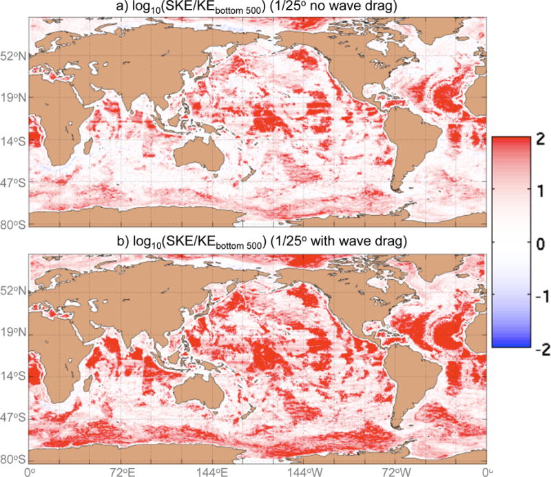
We next consider geographical distributions of baroclinicity. Figure 5 shows maps of KE_top100/KE_bot500 for the global mid- and strong-drag HYCOM simulations and Fig. 6 shows maps of the same quantity for the Atlantic mid- and weak-drag HYCOM simulations³). The locations where KE shows strong baroclinicity in the global maps of Fig. 5 tend to be within 40° of the equator or confined within bands in the Southern Ocean. Fig. 5 indicates that the number of grid points that are highly baroclinic is greater in the strong-drag simulation than in the mid-drag simulation, consistent with expectations from horizontally homogeneous QG turbulence simulations. In the weak drag simulations, baroclinicity is considerably reduced (compare Figs. 6a and 6b). Overall, baroclinicity of the KE in HYCOM behaves qualitatively as one might expect from from idealized, flat-bottom, horizontally homogeneous QG turbulence simulations: the flow becomes distinctly more barotropic with weak drag and more baroclinic with strong drag. An important difference from this classical picture is that surface and barotropic KE are individually less sensitive than is the case in classic studies of QG turbulence. This can be seen by inspection of Fig. 7, which displays KE_BT in the North Atlantic for the global and Atlantic HYCOM simulations with varying bottom drag strength. Although KE_BT is weaker when bottom drag is stronger (Fig. 7), this dependence is much less pronounced than is the signal as seen in baroclinicity (Figs. 5 and 6).

FIG. 5.

Shown are the base-10 logarithms of the ratios of the kinetic energy (KE) averaged over the top 100 meters to that averaged over the bottom 500 meters, each computed as a time average over the final year of (a) the mid-bottom drag 1/25° global HYCOM simulation and (b) the strong-bottom drag 1/25° global HYCOM simulation.

FIG. 6.

Shown are the base-10 logarithms of the ratios of the kinetic energy (KE) averaged over the top 100 meters to that averaged over the bottom 500 meters, each computed as a time average over (a) the final year of the mid-bottom drag 1/12° Atlantic HYCOM simulation and (b) the weak-bottom drag 1/12° Atlantic HYCOM simulation.

FIG. 7.

Shown is the base-10 logarithm of the barotropic kinetic energy, KE_BT (units in m² s⁻²), averaged over the final year of (a) the mid-bottom drag 1/25° global HYCOM simulation, (c) the strong-bottom drag 1/25° global HYCOM simulation, (b) the mid-bottom drag 1/12° Atlantic HYCOM simulation, and (d) the weak-bottom drag 1/12° Atlantic HYCOM simulation.

Our QG basin simulations allow us to examine the impacts of rough topography and lateral inhomogeneities on eddy statistics in QG flow. Fig. 8 displays the baroclinicity (quantified with both of the measures discussed earlier), as well as the surface and barotropic eddy horizontal length scales, in the QG basin simulations (with both rough and flat bottom topography), the previously reported horizontally homogeneous, two-layer, flat-bottom, f-plane, doubly periodic QG simulations of Arbic and Flierl (2004) and Arbic and Scott (2008), and the OGCM simulations. The abscissa of Fig. 8 represents the nondimensional friction strength, as defined by Arbic and Scott (2008) for the doubly periodic simulations, and defined by the ratio of the friction value to the nominal, or “control” value, for the QG basin and OGCM simulations. The QG basin simulations show that increased bottom drag leads to a more baroclinic flow, as expected (see blue curves in Figs. 8a-b), and in qualitative consistency with the QG turbulence results shown in Figs. 8a-b (black curves). Also as expected, overall there is less KE in the QG basin simulations when bottom drag strength is increased (Table 4).⁴ However, the sensitivity of baroclinicity and eddy energy to bottom drag strength is greatly reduced from what is seen in the horizontally homogeneous QG turbulence results, especially when rough topography is introduced into the QG basin simulations (e.g., compare the squares-solid blue curve to the diamonds-dot-dashed blue curve relative to the black curves in Figs. 8a-b, and the much greater sensitivity in Table 4 for the flat versus rough bottom simulations). This reduced sensitivity relative to horizontally homogeneous QG turbulence results is also seen in the HYCOM simulations over areas of rough topography, e.g., over a sub-domain of the North Atlantic (between 59.3° – 39.3°W and 19.6° – 39.6°N) close to the one shown in Fig. 1 (red curves in Figs. 8a-b). It seems clear that rough topography accounts for much of the discrepancy between our HYCOM simulations and expectations from classic studies of flat-bottom QG turbulence.

FIG. 8.

Shown are results from the horizontally homogeneous, two-layer, flat-bottom, f-plane, doubly periodic QG turbulence simulations with linear and quadratic bottom drags from Arbic and Flierl (2004) and Arbic and Scott (2008); the QG β-plane basin simulations with a flat bottom and rough bottom topography; and the 1/12° Atlantic and 1/25° global HYCOM simulations. We show non-dimensional eddy statistics: (a) the ratio of the domain-averaged kinetic energy (KE) in the top layer (subscript 1) to that in the bottom layer (subscript 2), (b) the domain-averaged ratio of the baroclinic KE to barotropic KE, (c) the domain-averaged ratio of the eddy length scales associated with KE in the barotropic mode (L_BT) to the Rossby radius of deformation (L_d), and (d) the domain-averaged ratio of the eddy length scales associated with KE in the upper layer (L₁) to L_d. A domain average has been taken over a region (between 59.3° –39.3°°W and 19.6° – 39.6°N) very close to the one shown in Fig. 1 for the 1/12° Atlantic and 1/25° global HYCOM simulations. Over this domain, L_d is assumed to be 30 km for not only the QG simulations, but also for the HYCOM simulations. The abscissa in each panel shows the nondimensional friction, as defined by Arbic and Scott (2008) for the doubly periodic QG simulations, and as defined by the relative magnitude of C_d or r_QG, with respect to the control simulation, for the HYCOM and QG basin simulations.

TABLE 4.

The domain-integrated kinetic energy (E_tot) [GJ= 10⁹J] in the quasi-geostrophic (QG) basin simulations with a flat bottom and rough bottom topography for three different values of linear bottom drag coefficients. The units of r_QG are in s⁻¹.

flat/rough topography	rQG	Etot
flat bottom	8 × 10−10	750
flat bottom	8 × 10−8	66
flat bottom	8 × 10−6	48
rough bottom	8 × 10−10	91
rough bottom	8 × 10−8	53
rough bottom	8 × 10−6	46

c. Surface eddy horizontal length scales

We next consider eddy horizontal length scales. In our HYCOM simulations, length scales L_KE associated with SKE are fairly insensitive to bottom drag strength (Fig. 8d; Table 5). Although we did not explicitly calculate a length scale for the KE in the barotropic mode of our HYCOM simulations, visual inspection of Fig. 7 suggests that it too is relatively insensitive to bottom drag strength. In contrast, the surface eddy horizontal length scales increase more dramatically with reducing drag strength in the weak-drag limit of the horizontally homogeneous, two-layer, flat-bottom, f-plane, doubly periodic QG turbulence results of Arbic and Flierl (2004) and Arbic and Scott (2008), as can be seen in Fig. 8d. The increase in surface length scales in these previous simulations is mainly due to an increase in the barotropic length scale (Fig. 8c).

TABLE 5.

The surface eddy horizontal length scales (L_KE) (units in km) associated with geostrophic surface kinetic energy computed over the final year of the 1/25° global HYCOM simulations and 1/12° Atlantic HY-COM simulations. The domain chosen for the entries listed here is the North Atlantic between 59.3° – 39.3°W and 19.6° – 39.6°N, very close to the region shown in Fig. 1.

configuration	Cd	wave drag?	LKE
1/12° Atlantic	5 × 10−4	no	50.4
1/12° Atlantic	2.5 × 10−3	no	52.0
1/25° global	2.5 × 10−3	no	56.7
1/25° global	2.5 × 10−1	no	53.8
1/25° global	2.5 × 10−3	yes	51.4

To investigate a possible reason for the weak sensitivity of HYCOM eddy horizontal length scales to bottom drag relative to flat-bottom, horizontally homogeneous QG turbulence results, we compare eddy length scales from our QG basin simulations with and without rough topography. We consider eddy length scales associated with barotropic KE (Fig. 8c) and surface, or upper layer, KE (Fig. 8d). As with the HYCOM simulations (red curves in Figs. 8d), there is no general trend for the eddy length scales as a function of bottom drag strength in our rough bottom QG basin simulations. However, the eddy length scales in the flat-bottom QG basin simulations behave more like the previous flat-bottom doubly periodic QG turbulence results – both barotropic and surface eddy length scales increase greatly as drag is weakened in the weak drag limit. Overall, our results suggest that rough topography reduces the sensitivity of eddy horizontal length scales to bottom drag. This insensitivity can be visualized through examination of snapshots of the upper layer streamfunction, shown in Fig. 9, for the QG basin simulations. The flat bottom simulations show large qualitative differences as drag strength is altered. With rough topography, this sensitivity is markedly reduced. In addition, we note that the presence of topography matters less to the surface streamfunction when the drag is strong. For instance, the streamfunctions for the simulations with strong-drag in flat- and rough-bottom configurations (Figs. 9c and 9f, respectively) are more similar to each other than are the streamfunctions for the simulations with mid- or weak-drag in flat- and rough-bottom configurations (Figs. 9a,d and 9b,e). This is because the bottom horizontal flow, $\overrightarrow{u}$, approaches zero in the strong-drag regime, and the impact of topography on QG flows is proportional to $\overrightarrow{u}\cdot \nabla h$, where h is the bottom topography. Our QG basin simulation results are consistent with the finding from previous studies (e.g., Nadeau et al., 2013) that use of realistic rough topography increases baroclinicity (e.g., compare upper and lower layer kinetic energies in their Table 2).

FIG. 9.

Shown are representative snapshots of the streamfunction (units in m² s⁻¹) in the top layer of the QG β-plane basin simulations with (a-c) a flat bottom and (d-f) rough bottom topography. The simulations use a linear bottom drag coefficient of (a,d) 8 × 10⁻¹⁰ s⁻¹, (b,e) 8 × 10⁻⁸ s⁻¹, and (c,f) 8 × 10⁻⁶ s⁻¹. The axes have the same latitude and longitude labels as in Fig. 1.

It seems clear that rough topography acts to reduce the sensitivity of eddy horizontal length scales to bottom drag strength. Other differences between our HYCOM simulations and many classic studies of QG turbulence include vertical resolution (e.g., the number of layers, which is often only two in QG turbulence models); horizontal inhomogeneities; and other modeling choices, such as the choice of linear versus quadratic parameterizations of bottom drag. Although it is difficult to make a direct comparison, the use of a quadratic bottom drag instead of a linear drag may also account for part of the weakened sensitivity in HYCOM. Arbic and Scott (2008) showed that the sensitivities in QG turbulence to linear drag are greater than those for quadratic drag, as can be seen in Fig. 8 here. It seems unlikely that the reduced sensitivity seen in our HYCOM simulations (relative to classic studies) is strongly affected by vertical resolution, ageostrophic dynamics, or horizontal inhomogeneity. In support of this statement, we note that Hurlburt et al. (2008) used a realistic OGCM similar to HYCOM, but with a flat bottom. They find much larger changes in mean SSH in response to changes in bottom drag than we see, despite the inclusion of horizontal inhomogeneity, ageostrophic dynamics, and higher vertical resolution in their model.

A working hypothesis for why rough topography acts to reduce the sensitivity of eddy horizontal length scales to bottom drag is that barotropization of baroclinic energy gets short-circuited in the presence of rough bottom topography. Barotropization of baroclinic energy extracts baroclinic energy from scales near the deformation radius and injects it into the barotropic mode, typically at somewhat larger horizontal scales. This energy remains resident in the barotropic mode, essentially until it is removed by bottom friction. With rough topography, much of this barotropic energy can be transferred back to the baroclinic mode; that is, interaction between topography and the barotropic streamfunction forces the baroclinic mode. Assuming this to occur at a comparable or faster rate than the rate at which bottom drag acts to remove barotropic energy, the barotropization process becomes effectively “short-circuited”. Our hypothesis and those posed by previous studies (e.g., Hurlburt et al., 2008) on the influence of rough topography on eddying flows would explain the relatively small changes observed in geostrophic SKE, SSH variance, and eddy horizontal length scales here.

d. Effect of wave drag

The strong and weak values of bottom drag used here help to demonstrate the impact of bottom drag strength on eddy statistics, but these extreme drag values lie outside of physically plausible limits. Aside from the “mid” value of C_d = 2.5×10⁻³, an additional plausible momentum sink in the ocean is that associated with wave drag, as described in Trossman et al. (2013, 2016). Here, we briefly investigate whether the sensitivity of eddy statistics to the presence of a physically plausible wave drag momentum sink is qualitatively similar to the sensitivity seen with the extremes of bottom drag strength discussed in previous sections.

Including wave drag and boosting bottom drag strength impact HYCOM in a qualitatively similar manner. The near-bottom flows are also weakened in the HYCOM simulation with wave drag such that the vertical profile of KE is more baroclinic relative to the simulation without wave drag (Fig. 10; Table 3; Trossman et al., 2016 - their Figs. 11a-d). As with the sensitivity of HYCOM eddy length scales to bottom drag strength (Fig. 8d; Table 5), L_KE in HYCOM is fairly insensitive to the presence of wave drag (Table 5). Area-averaged SSH variance and geostrophic SKE in HYCOM are both sensitive at the ∼20% level to the inclusion of wave drag (Trossman et al., 2016 - their Figs. 5 and 7; their Table 2; also see Table 2 in this paper). Lastly, the conversion rate between kinetic and potential energy must change with the same sign when wave drag is included as when bottom drag strength is increased.

FIG. 10.

Shown are the base-10 logarithms of the ratios of the geostrophic surface kinetic energy (KE) to the KE averaged over the bottom 500 meters, each computed as a time average over the final year of (a) the mid-bottom drag 1/25° global HYCOM simulation without wave drag and (b) the 1/25° global HYCOM simulation with wave drag.

The responses of the HYCOM simulations with wave drag and strong bottom drag, however, are not identical. When wave drag is included, the SSH variance and geostrophic SKE are actually decreased, in contrast to the slight increases seen with increasing bottom drag (Table 2). This demonstrates the fundamentally different physical consequences of including wave drag relative to boosting bottom drag. Here we surmise that the spatially varying coefficient, r_drag, in the wave drag parameterization is the source of the qualitatively different responses of SSH variance and geostrophic SKE to the presence of wave drag as opposed to increasing bottom drag strength. From the results of Hurlburt and Hogan (2008), who varied bottom drag strength using only six layers in the vertical direction and a flat bottom in a model very similar to HYCOM, we suggest that applying a bottom drag over a much larger bottom layer thickness than in our HYCOM simulations would not cause qualitatively different behavior in the geostrophic SKE and SSH variance. We also suggest, based upon the horizontally homogeneous QG turbulence results of Arbic and Scott (2008), that using a linear, as opposed to quadratic, bottom drag near the seafloor is not the cause of the qualitatively different behaviors seen when using wave drag versus bottom drag.

5. Conclusions

The present study investigates the sensitivity of midocean eddy statistics to bottom drag, rough topography, and wave drag in models of varying complexity. A primary focus is on whether the conclusions drawn from horizontally homogeneous, two-layer, flat-bottom, f-plane, doubly periodic QG turbulence simulations about sensitivity to bottom drag (e.g., Arbic and Flierl, 2004; Arbic and Scott, 2008) qualitatively apply to more realistic ocean models. In the QG basin and realistic OGCM simulations with strong bottom drag studied here, the KE is reduced in the bottommost layer and generally becomes more baroclinic, as in the earlier two-layer doubly periodic QG results. As a result, the agreement with the vertical structure, or baroclinicity, of eddy KE in current meter observations is better for the OGCM simulations with a nominal “mid” value of bottom drag than for the OGCM simulations with a strong bottom drag. In the QG basin and OGCM simulations with weak bottom drag studied here, the KE becomes more barotropic, again in accordance with earlier two-layer doubly periodic QG results. However, the sensitivity of the baroclinicities in the QG basin simulations to bottom drag is reduced for rough bottom conditions relative to flat bottom conditions, suggesting that rough topography mediates the sensitivity of baroclinicity to bottom drag.

The qualitative results about the horizontal eddy length scales seen in horizontally homogeneous, two-layer, flat-bottom, f-plane, doubly periodic QG turbulence damped by very weak or strong bottom drag are not seen in the QG basin simulations performed here with rough topography. In line with earlier results (e.g., Treguier and Hua, 1988), the use of rough topography reduces the sensitivity of eddy horizontal length scales to bottom drag strength in QG basin simulations. Our QG basin simulations suggest that the bathymetry of the more realistic OGCM simulations is partially responsible for the relatively weak impact of bottom drag or wave drag on horizontal eddy length scales.

References

- Abernathey R, Cessi P. Topographic enhancement of eddy efficiency in baroclinic equilibration. J Phys Oceanogr. 2014;44:2107–2126. [Google Scholar]
- Andersen OB, Knudsen P. The DNSC08 mean sea surface and mean dynamic topography. J Geophys Res-Oceans. 2009;114:C11. doi: 10.1029/2008JC005179. [DOI] [Google Scholar]
- Andersen OB. The DTU10 Gravity field and Mean sea surface, Second international symposium of the gravity field of the Earth (IGFS2) Fairbanks, Alaska: 2010. [Google Scholar]
- Arbic BK, Flierl GR. Baroclinically unstable geostrophic turbulence in the limits of strong and weak bottom Ekman friction: application to midocean eddies. J Phys Oceanogr. 2004;34:2257–2273. [Google Scholar]
- Arbic BK, Flierl GR, Scott RB. Cascade inequalities for forced-dissipated geostrophic turbulence. J Phys Oceanogr. 2007;37:1470–1487. [Google Scholar]
- Arbic BK, Scott RB. On quadratic bottom drag, geostrophic turbulence, and oceanic mesoscale eddies. J Phys Oceanogr. 2008;38:84–103. [Google Scholar]
- Arbic BK, Shriver JF, Hogan PJ, Hurlburt HE, McClean JL, Metzger EJ, Scott RB, Sen A, Smedstad OM, Wallcraft AJ. Estimates of bottom flows and bottom boundary layer dissipation of the oceanic general circulation from global high-resolution models. J Geophys Res. 2009;114:C02024. [Google Scholar]
- Arbic BK, Scott RB, Chelton DB, Richman JG, Shriver JF. Effects of stencil width on surface ocean geostrophic velocity and vorticity estimation from gridded satellite altimeter data. J Geophys Res-Oceans. 2012;117:C03029. [Google Scholar]
- Arbic BK, Polzin KL, Scott RB, Richman JG, Shriver JF. On eddy viscosity, energy cascades, and the horizontal resolution of gridded satellite altimeter products. J Phys Oceanogr. 2013;43:283–300. [Google Scholar]
- Arbic BK, Müller M, Richman JG, Shriver JF, Morten AJ, Scott RB, Sérazin G, Penduff T. Geostrophic turbulence in the frequency-wavenumber domain: eddy-driven low-frequency variability. J Phys Oceanogr. 2014;44:2050–2069. [Google Scholar]
- Baines PG. Topographic effects in stratified flows. Cambridge Univ Press; Cambridge, U K: 1995. [Google Scholar]
- Benilov ES, Nycander J, Dritschel DG. Destabilization of barotropic flows by small-scale topography. J Fluid Mech. 2004;517:359–374. [Google Scholar]
- Bleck R. An oceanic general circulation model framed in hybrid isopycnic-Cartesian coordinates. Ocean Modelling. 2002;37:55–88. [Google Scholar]
- Boland EJD, Thompson AF, Shuckburgh E, Haynes PH. The formation of nonzonal jets over sloped topography. J Phys Oceanogr. 2012;42:1635–1651. [Google Scholar]
- Brüggemann N, Eden C. Routes to dissipation under different dynamical conditions. J Phys Oceanogr. 2015;45:2149–2168. [Google Scholar]
- Chassignet EP, Garraffo ZD. Viscosity parameterization and the Gulf Stream separation. In “From Stirring to Mixing in a Stratified Ocean”. In: Muller P, Henderson D, editors. Proceedings of the 12th ’Aha Huliko’a Hawaiian Winter Workshop U of Hawaii. 2001. pp. 37–41. [Google Scholar]
- Chassignet EP, Smith LT, Halliwell GR, Bleck R. North Atlantic simulations with the Hybrid Coordinate Ocean Model (HYCOM): impact of the vertical coordinate choice, reference pressure, and thermobaricity. J Phys Oceanogr. 2003;33:2504–2526. [Google Scholar]
- Chassignet EP, Hurlburt HE, Smedstad OM, Halliwell GR, Wallcraft AJ, Metzger EJ, Blanton BO, Lozano C, Rao DB, Hogan PJ, Srinivasan A. Generalized vertical coordinates for eddy-resolving global and coastal ocean forecasts. Oceanography. 2006;19(1):20–31. [Google Scholar]
- Chassignet EP, Marshall DP. Gulf Stream separation in numerical ocean models. In: Hecht M, Hasumi H, editors. Eddy-Resolving Ocean Modeling. 2008. pp. 39–62. (AGU Monograph Series). [Google Scholar]
- Chassignet EP, Hurlburt HE, Metzger EJ, Smedstad OM, Cummings JA, Halliwell GR, Bleck R, Baraille R, Wallcraft AJ, Lozano C, Tolman HL, Srinivasan A, Hankin S, Cornillon P, Wesberg R, Barth A, He R, Werner F, Wilkin J. US GODAE global ocean prediction with the HYbrid Coordinate Ocean Model (HYCOM) Oceanography. 2009;22(2):64–75. Sp. Iss. SI. [Google Scholar]
- Chelton DB, Schlax MG, Samelson RM. Global observations of nonlinear mesoscale eddies. Prog Oceanogr. 2011;91:167–216. [Google Scholar]
- Chen C, Kamenkovich I. Effects of topography on baroclinic instability. J Phys Oceanogr. 2013;43:790–804. [Google Scholar]
- Chen C, Kamenkovitch I, Berloff P. On the dynamics of flows induced by topographic ridges. J Phys Oceanogr. 2015;45:927–940. [Google Scholar]
- Dewar W. Topography and barotropic transport control by bottom friction. J Mar Res. 1998;56:295–328. [Google Scholar]
- Feddersen F, Gallagher EL, Guza RT, Elgar S. The drag coefficient, bottom roughness, and wave-breaking in the nearshore. Coast Engin. 2003;48:189–195. [Google Scholar]
- Garner ST. A topographic drag closure built on an analytical base flux. J Atmos Sci. 2005;62:2302–2315. [Google Scholar]
- Griffies SM, Böning C, Bryan FO, Chassignet EP, Gerdes R, Hasumi H, Hirst A, Treguier AM, Webb D. Developments in ocean climate modelling. Ocean Modelling. 2000;2:123–192. [Google Scholar]
- Haidvogel DB, Held IM. Homogeneous quasigeostrophic turbulence driven by a uniform temperature gradient. J Atmos Sci. 1980;37:2644–2660. [Google Scholar]
- Halliwell GR. Evaluation of vertical coordinate and vertical mixing algorithms in the HYbrid-Coordinate Ocean Model (HYCOM) Ocean Modelling. 2004;7:285–322. [Google Scholar]
- Hogg AMcC, Blundell JR. Interdecadal Variability of the Southern Ocean. J Phys Oceanogr. 2006;36:1626–1645. [Google Scholar]
- Hurlburt HE, Hogan PJ. The Gulf Stream pathway and the impacts of the eddy-driven abyssal circulation and the Deep Western Boundary Current. Dyn Atmos Ocean. 2008;45:71–101. [Google Scholar]
- Hurlburt HE, Metzger EJ, Hogan PJ, Tilburg CE, Shriver JF. Steering of upper ocean currents and fronts by the topographically constrained abyssal circulation. Dyn Atmos Ocean. 2008;45:102–134. [Google Scholar]
- Kallberg P, Simmons A, Uppala S, Fuentes M. The ERA-40 Archive. ECMWF; 2004. (ERA-40 Project Report Series No 17). [Google Scholar]
- Kelly KA, Thompson L, Cheng W, Metzger EJ. Evaluation of HYCOM in the Kuroshio Extension region using new metrics. J Geophys Res-Oceans. 2007;112:C01004. [Google Scholar]
- LaCasce JH, Brink KH. Geostrophic turbulence over a slope. J Phys Oceanogr. 2000;30:1305–1324. [Google Scholar]
- Large WG, McWilliams JC, Doney SC. Oceanic vertical mixing: a review and a model with a nonlocal boundary layer parameterization. Rev Geophys. 1994;32:363–403. [Google Scholar]
- Larichev VD, Held IM. Eddy amplitudes and fluxes in a homogeneous model of fully developed baroclinic instability. J Phys Oceanogr. 1995;25:2285–2297. [Google Scholar]
- Merryfield WJ. Effects of stratification on quasi-geostrophic inviscid equilibria. J Fluid Mech. 1998;354:345–356. [Google Scholar]
- Nadeau LP, Straub DN. Influence of wind stress, wind stress curl, and bottom friction on the transport of a model Antarctic Circumpolar Current. J Phys Oceanogr. 2012;42:207–222. [Google Scholar]
- Nadeau LP, Straub DN, Holland DM. Comparing idealized and complex topographies in quasigeostrophic simulations of an Antarctic Circumpolar Current. J Phys Oceanogr. 2013;43:1821–1837. [Google Scholar]
- Nadeau LP, Ferrari R. The role of closed gyres in setting the zonal transport of the Antarctic Circumpolar Current. J Phys Oceanogr. 2015;45:1491–1509. [Google Scholar]
- Naveira-Garabato AC, Nurser AJG, Scott RB, Goff JA. The impact of small-scale topography on the dynamical balance of the ocean. J Phys Oceanogr. 2013;43:647–668. [Google Scholar]
- Nikurashin M, Ferrari R. Global energy conversion rate from geostrophic flows into internal lee waves in the deep ocean. Geophys Res Lett. 2011;38:L08610. [Google Scholar]
- Olbers D, Borowski D, Völker C, Wolff J-O. The dynamical balance, transport and circulation of the Antarctic Circumpolar Current. Antarctic Science. 2004;16(4):439–470. [Google Scholar]
- Özgökmen T, Chassignet EP. Emergence of inertial gyres in a two-layer quasi-geostrophic model. J Phys Oceanogr. 1998;28:461–484. [Google Scholar]
- Qiu B, Scott RB, Chen S. Length scales of eddy generation and nonlinear evolution of the seasonally modulated South Pacific Subtropical Countercurrent. J Phys Oceanogr. 2008;38:1515–1528. [Google Scholar]
- Radko T, Peixoto de Carvalho D, Flanagan J. Nonlinear equilibration of baroclinic instability: the growth rate balance model. J Phys Oceanogr. 2014;44:1919–1940. [Google Scholar]
- Rhines PB. Edge-, bottom-, and Rossby waves in a rotating stratified fluid. Geophys Fluid Dyn. 1970;1:273–302. [Google Scholar]
- Rhines P. The dynamics of unsteady currents. The Sea, Interscience. 1977;6:189–318. [Google Scholar]
- Riviere P, Treguier AM, Klein P. Effects of bottom friction on nonlinear equilibration of an oceanic baroclinic jet. J Phys Oceanogr. 2004;34:416–432. [Google Scholar]
- Rosmond TE, Teixeira J, Peng M, Hogan TF, Pauley R. Navy Operational Global Atmospheric Prediction System (NOGAPS): forcing for ocean models. Oceanography. 2002;15:99–108. [Google Scholar]
- Salmon R. Two-layer quasi-geostrophic turbulence in a simple special case. Geophys Astrophys Fluid Dyn. 1978;10:25–52. [Google Scholar]
- Salmon R. Baroclinic instability and geostrophic turbulence. Geophys Astrophys Fluid Dyn. 1980;15:167–211. [Google Scholar]
- Schlösser F, Eden C. Diagnosing the energy cascade in a model of the North Atlantic. Geophys Res Lett. 2007;34:L02604. doi: 10.1029/2006GL027813. [DOI] [Google Scholar]
- Scott RB, Wang F. Direct evidence of an oceanic inverse kinetic energy cascade from satellite altimetry. J Phys Oceanogr. 2005;35:1650–1666. doi: 10.1175/JPO2771.1. [DOI] [Google Scholar]
- Scott RB, Arbic BK. Spectral energy fluxes in geostrophic turbulence: Implications for ocean energetics. J Phys Oceanogr. 2007;37:673–688. doi: 10.1175/JPO3027.1. [DOI] [Google Scholar]
- Scott RB, Arbic BK, Chassignet EP, Coward AC, Maltrud M, Merryfield WJ, Srinivasan A, Varghese A. Total kinetic energy in four global eddying ocean circulation models and over 5000 current meter records. Ocean Modelling. 2010;32:157–169. [Google Scholar]
- Scott RB, Goff JA, Naveira-Garabato AC, Nurser AJG. Global rate and spectral characteristics of internal gravity wave generation by geostrophic flow over topography. J Geophys Res. 2011;116:C09029. doi: 10.1029/2011JC007005. [DOI] [Google Scholar]
- Sen A, Scott RB, Arbic BK. Global energy dissipation rate of deep-ocean low-frequency flows by quadratic bottom boundary layer drag: computations from current-meter data. Geophys Res Lett. 2008;35:L09606. doi: 10.1029/2008GL033407. [DOI] [Google Scholar]
- Sinha B, Richards KJ. Jet structure and scaling in Southern Ocean models. J Phys Oceanogr. 1999;29:1143–1155. [Google Scholar]
- Smagorinsky J. Large eddy simulation of complex engineering and geophysical flows. In: Galperin B, Orszag SA, editors. Evolution of Physical Oceanography. Cambridge University Press; 1993. pp. 3–36. [Google Scholar]
- Smith WHF, Sandwell DT. Global seafloor topography from satellite altimetry and ship depth soundings. Science. 1997;277:1957–1962. [Google Scholar]
- Srinivasan A, Garraffo Z, Iskandarani M. Abyssal circulation in the Indian Ocean from a 1/12° resolution global hindcast. Deep-Sea Res I. 2009;56:1907–1926. [Google Scholar]
- Stammer D. Global characteristics of ocean variability estimated from regional TOPEX/Poseidon altimeter measurements. J Phys Oceanogr. 1997;27:1743–1769. [Google Scholar]
- Stewart KD, Saenz JA, Hogg AMcC, Hughes GO, Griffiths RW. Effect of topographic barriers on the rates of available potential energy conversion of the oceans. Ocean Modelling. 2014;76:31–42. [Google Scholar]
- Straub DN, Nadiga BT. Energy fluxes in the quasigeostrophic double gyre problem. J Phys Oceanogr. 2014;44:1505–1522. [Google Scholar]
- Taylor GI. Tidal friction in the Irish Sea. Philos Trans R Soc London, Ser A. 1919;220:1–33. [Google Scholar]
- Thompson AF. Jet formation and evolution in baroclinic turbulence with simple topography. J Phys Oceanogr. 2010;40:257–278. [Google Scholar]
- Thompson AF, Young WR. Scaling baroclinic eddy fluxes: vortices and energy balance. J Phys Oceanogr. 2006;36:720–738. [Google Scholar]
- Thoppil PG, Richman JG, Hogan PJ. Energetics of a global ocean circulation model compared to observations. Geophys Res Lett. 2011;38:L15607. doi: 10.1029/2011GL048347. [DOI] [Google Scholar]
- Timko PG, Arbic BK, Richman JG, Scott RB, Metzger EJ, Wallcraft AJ. Skill testing a three-dimensional global tide model to historical current meter records. J Geophys Res-Oceans. 2013;118:6914–6933. doi: 10.1002/2013JC009071. [DOI] [Google Scholar]
- Treguier AM, Hua BL. Influence of bottom topography on stratified quasi-geostrophic turbulence in the ocean. Geophys Astrophys Fluid Dyn. 1988;43:265–305. [Google Scholar]
- Treguier AM, McWilliams JC. Topographic influences on wind-driven, stratified flow in a β-plane channel: An idealized model for the Antarctic Circumpolar Current. J Phys Oceanogr. 1990;20:321–343. [Google Scholar]
- Trossman DS, Arbic BK, Garner ST, Goff JA, Jayne SR, Metzger EJ, Wallcraft AJ. Impact of parameterized lee wave drag on the energy budget of an eddying global ocean model. Ocean Modelling. 2013;72:119–142. [Google Scholar]
- Trossman DS, Waterman S, Polzin KL, Arbic BK, Garner ST, Naveira-Garabato AC, Sheen KL. Internal lee wave closures: parameter sensitivity and comparison to observations. J Geophys Res-Oceans. 2015;120 doi: 10.1002/2015JC010892. [DOI] [Google Scholar]
- Trossman DS, Arbic BK, Richman JG, Garner ST, Jayne SR, Wallcraft AJ. Impact of topographic internal lee wave drag on an eddying global ocean model. Ocean Modelling. 2016;97:109–128. [Google Scholar]
- Trowbridge JH, Geyer WR, Bowen MM, Williams AJ. Near-bottom turbulence measurements in a partially mixed estuary: turbulent energy balance, velocity structure, and along-channel momentum balance. J Phys Oceanogr. 1999;29:3056–3072. [Google Scholar]
- Trowbridge J, Elgar S. Turbulence measurements in the surf zone. J Phys Oceanogr. 2001;31:2403–2417. [Google Scholar]
- Tulloch R, Marshall J, Hill C, Smith KS. Scales, growth rates, and spectral fluxes of baroclinic instability in the ocean. J Phys Oceanogr. 2011;41:1057–1076. [Google Scholar]
- Uppala SM, Kallberg PW, Simmons AJ, Andrae U, Da Costa Bechtold V, Fiorino M, Gibson JK, Haseler J, Hernandez A, Kelly GA, Li X, Onogi K, Saarinen S, Sokka N, Allan RP, Andersson E, Arpe K, Balmaseda MA, Beljaars ACM, Van De Berg L, Bidlot J, Bormann N, Caires S, Chevallier F, Dethof A, Dragosavac M, Fisher M, Fuentes M, Hagemann S, Holm E, Hoskins BJ, Isaksen L, Janssen PAEM, Jenne R, Mcnally AP, Mahfouf J-F, Morcrette J-J, Rayner NA, Saunders RW, Simon P, Sterl A, Trenberth KE, Untch A, Vasiljevic D, Viterbo P, Woollen J. The ERA-40 renalaysis. Q J R Meteorol Soc. 2005;131:2961–3012. doi: 10.1256/qj.04.176. [DOI] [Google Scholar]
- Venaille A, Vallis GK, Smith KS. Baroclinic turbulence in the ocean: analysis with primitive equation and quasigeostrophic simulations. J Phys Oceanogr. 2011;41:1605–1623. [Google Scholar]
- Venaille A. Bottom-trapped currents as statistical equilibrium states above topographic anomalies. J Fluid Mech. 2012;699:500–510. [Google Scholar]
- Weatherly GL. A numerical study of time-dependent turbulent Ekman layers over horizontal and sloping bottoms. J Phys Oceanogr. 1975;5:288–299. [Google Scholar]
- Willebrand W, Barnier B, Boning C, Dieterich C, Killworth PD, Le Provost C, Jia Y, Molines JM, New AL. Circulation characteristics in three eddy-permitting models of the North Atlantic. Progr Oceanogr. 2001;48:123–161. [Google Scholar]
- Wright CJ, Scott RB, Furnival D, Ailliot P, Vermet F. Global Observations of Ocean-Bottom Subinertial Current Dissipation. J Phys Oceanogr. 2013;43:402–417. [Google Scholar]
- Wright CJ, Scott RB, Ailliot P, Furnival D. Lee wave generation rates in the deep ocean. Geophys Res Lett. 2014;41 doi: 10.1002/2013GL059087. [DOI] [Google Scholar]
- Wunsch C. The vertical partition of oceanic horizontal kinetic energy. J Phys Oceanogr. 1997;27:1770–1794. [Google Scholar]
- Xu X, Rhines PB, Chassignet EP. Temperature-salinity structure of the North Atlantic circulation and associated heat and freshwater transports. J Clim. 2016 doi: 10.1175/JCLI-D-15-0798.1. [DOI] [Google Scholar]