On computational fluid dynamics models for sinonasal drug transport: relevance of nozzle subtraction and nasal vestibular dilation

SUMMARY

Generating anatomically realistic three-dimensional (3D) models of the human sinonasal cavity for numerical investigations of sprayed drug transport presents a host of methodological ambiguities. For example, subject-specific radiographic images used for 3D reconstructions typically exclude spray bottles. Subtracting a bottle contour from the 3D airspace and dilating the anterior nasal vestibule for nozzle placement augment the complexity of model-building. So, we explored the question: how essential are these steps to adequately simulate nasal airflow and identify the optimal delivery conditions for intranasal sprays? In particular, we focused on particle deposition patterns in the maxillary sinus, a critical target site for chronic rhinosinusitis (CRS). The models were reconstructed from post-surgery computed tomography scans for a 39-year-old Caucasian male, with CRS history. Inspiratory airflow patterns during resting breathing are reliably tracked through CFD-based steady state laminar-viscous modeling and such regimes portray relative lack of sensitivity to inlet perturbations. Consequently, we hypothesized that the posterior airflow transport and the particle deposition trends should not be radically affected by the nozzle subtraction and vestibular dilation. The study involved 1 base model and 2 derived models; the latter two with nozzle contours (two different orientations) subtracted from the dilated anterior segment of the left vestibule. We analyzed spray transport in the left maxillary sinus for multiple release conditions. Similar release points, localized on an approximately 2mm-by-4.5mm contour, facilitated improved maxillary deposition in all three test cases. This suggests functional redundancy of nozzle insertion in a 3D numerical model for identifying the optimal spray release locations.

Graphical abstract

Identifying optimal intranasal spray release points through CFD modeling presents methodological ambiguities on the inclusion of spray nozzle in the CT-based 3D reconstructions. We simulated spray transport in three anatomically realistic models from the same subject: one base model, and two derived models with lateral vestibular dilation and nozzle subtraction in two different orientations. Similar release points facilitated improved target site particle deposition (TSPD) in all three test models, indicating that TSPD trends are less sensitive to nozzle-induced inlet perturbations.

1. INTRODUCTION

Therapeutics for chronic rhinosinusitis (CRS) constitutes a layered approach^1–4 comprising oral antibiotics, anti-inflammatory drugs, and surgical intervention, along with topical medications like nasal sprays. The anatomical alteration through surgery does not always address the inflammation from CRS, while long-term use of antibiotics and anti-inflammatory medications comes with systemic side-effects. Consequently, topical nasal sprays may represent a viable component of medical therapy for CRS. There is, however, a caveat as the topical sprays do not always ensure an optimal drug delivery to the affected areas of the sinonasal cavity. Of interest is hence to identify the different spray parameters and application techniques that would maximize the topical deposition of the drugs in critical areas like the maxillary and the ethmoid sinuses (see Figure 1 for these anatomical landmarks). The techniques entail the head positions, nozzle positions, and breathing methods that would maximize the target site particle deposition (TSPD). While in vivo measurements of drug delivery is an ambitious idea, computational fluid dynamics (CFD) simulations of nasal spray intake promise a feasible preliminary path towards identification of the optimal spray techniques.

Figure 1.

(a) A representative CT imaging slice of the subject’s sinonasal cavity, after a bilateral functional endoscopic sinus surgery. The coronal section is at the level of mid maxillary sinus. Panel (b) depicts the coronal view and panel (c) presents the sagittal view of the anatomically realistic 3D reconstruction of the sinonasal cavity from the CT scans. The different sinonasal chambers are marked.

Investigations through the CFD route incorporate the following three basic steps: (1) acquiring the patient-specific computed tomography (CT) scans of the sinonasal cavity, (2) developing an in silico three-dimensional (3D) sinonasal model based on the CT scans using an image-processing software package, and creating a mesh of the flow domain for numerical simulations, (3) CFD analysis of the meshed model using numerical discretization techniques. Step (3) outputs the topical deposition of the medicated particles by tracking the flow patterns and the particle trajectories. To run a reliable simulation, it might seem essential to insert a nozzle into the 3D model in step (2) and edit the model by subtracting the nozzle contour from the nasal airspace, along with dilating the lateral walls to account for nozzle placement. The tip of the nozzle would indicate the starting point of the nasal spray particle transport. However, the patient-specific scans typically exclude any nozzle, and insertion of a nozzle at the image-processing stage involves an elaborate superficial reshaping of the anterior nasal cavity lining. There is no conclusive evidence in literature on the variability of the CFD-based modeling strategy to identify the optimal nasal spray instructions, based on whether the spray nozzle is accounted for or not in the CT-based 3D reconstructions. Some^5–7 do not incorporate any spray device in their computational models, while others^{8, 9} who have considered inserted nozzles, did not include sinuses in their nasal models. A recent preliminary study¹⁰ (presented at the International Society for Aerosols in Medicine [ISAM] Congress in Munich, Germany, May–June 2015) in the sinus-less model of one normal subject however suggested that the regional particle deposits were largely unaffected by the nozzle presence.

To address the above ambiguity and to expedite the 3D modeling protocol, our study presents a comparison of the TSPD trends of nasal spray particles in three different test models (1 base model and 2 additional derived models) developed from the CT scans of the same patient. The models differed only at the anterior part of the nasal cavity at the left nostril. Model I (base model; see Figure 2(a)) did not include any nozzle, while Model II and Model III (see panels (b) and (c) in Figure 2) included spray bottles with two very different nozzle orientations (subtracted from the internal airspace), while still making sure that the spray directions conformed to the clinical safety guidelines.¹¹

Figure 2.

(a) Model I (base model) reconstructed from the CT scans. Panels (b) and (c) show the derived models (Model II and Model III, respectively). In (b) and (c), the red contours comprise the nozzle-subtracted airspace and represent two different nozzle orientations. Note that although the outer lining of the nozzle contour touched the nasal wall in Models II and III, still the nozzle tip remained in the internal cavity space in each case. Panel (d) demonstrates the real nozzle contour that was subtracted from the base model airspace to generate Models II and III.

Nasal airflow for resting breathing has been evidenced to be predominatly laminar,^12–14 implying that the flow features are less sensitive to the inlet-zone perturbations resulting from the nozzle insertion in the anterior nasal vestibule. Thus, we hypothesized that the posterior airflow transport and consequently the sprayed particle depostion patterns in the three models should be relatable, which would in turn suggest redundacy of nozzle insertion in the numerical models while trying to identify the optimal spray release conditions. To check this hypothesis, we conducted particle simulations for a wide array of release points in the left nasal airspace and compared the locations for improved topical deposition in the left maxillary sinus (LMS) across the three test models. A preliminary report on this work was presented¹⁵ at the annual meeting of the American Physical Society (APS) Division of Fluid Dynamics Meeting in Portland, OR, November 2016.

2. METHODS

2.1. Patient selection

This methods study was implemented under the approval of the Institutional Review Board (IRB) committee at the University of North Carolina at Chapel Hill. It is part of an ongoing more extensive investigation¹⁶ by our group to identify the optimal spray techniques and breathing methods for improved topical deposition of medicated aerosol particles, using the tools of CFD, supplemented by in vitro experimental findings. We are aiming for a final cohort recruitment of 30 CRS patients. The acquired CT scans, before and after functional endoscopic sinus surgery (FESS), would be used to develop 3D models for CFD-based explorations. In order to ensure a homogeneous study population, we only include patients without polyps and with the sinus disease confined primarily to the ostiomeatal complex (OMC). For the current study, we have used de-identified CT scans from a 39-year-old Caucasian male (weighing 94.5 kg with height 72 inches), who had a bilateral FESS for the treatment of medically recalcitrant CRS, without nasal polyps.

2.2. Model geometry and meshing

2.2.1. Generating the base sinonasal model (Model I)

Anatomically realistic 3D reconstruction of the sinonasal airspace was developed from the post-operative CT scan images imported into the medical imaging software package Mimics™ 18.0 (Materialize, Inc., Plymouth, MI, USA) in Digital Imaging and Communications in Medicine (DICOM) file format. The scans consisted of 270 slices, taken at depth increments of 0.399 mm, with a pixel size of 0.4 mm. An image radiodensity threshold range of −1024 to −300 Hounsfield units¹⁷ was used to delineate the nasal airways and the paranasal sinuses from the medical-grade CT scans, followed by careful hand-editing of the selected pixels to achieve anatomic accuracy. The sinonasal geometries were exported in stereolithography (STL) file format to the computer-aided design and meshing software ICEM-CFD™ 15.0 (ANSYS, Inc., Canonsburg, PA, USA), where the 3D reconstruction was finalized in an XYZ cartesian space. For convenience, all the geometries were re-oriented in ICEM™ to render the nasal floor parallel to the Z axis. For the airspace boundaries: (1) planar surfaces were added spanning the outer rims of the nostrils, (2) a 2-cm outlet tube was added to the posterior end of the nasopharynx to ensure a fully-developed outlet flow and was closed off by a planar surface. Figure 2(a) displays the digital 3D rendition of the base sinonasal model (Model I). Note that the posterior outlet tube was not shown in this visual, to zoom in on the finer nuances of the models.

2.2.2. Establishing the meshing parameters for grid-independence

Based on a sensitivity analysis¹⁸ on the average pressure at the posterior septum and on the outlet flow, it was previously demonstrated that four million graded tetrahedral elements in the base computational mesh of a nasal model were sufficient to achieve robust and grid-independent numerical solutions. However, sensitivity of the simulations towards localized mesh refinement of the target anatomical sites was still unexplored. To probe further on this methodological uncertainty, we implemented refinements on the base mesh in the maxillary sinuses to generate four additional meshed models along with the base computational mesh (with four million graded tetrahedral elements). The number of tetrahedral elements in the two maxillary sinuses for the four locally mesh-refined models were respectively 1.5 times, 2 times, 2.5 times, and 3 times the number of elements in the maxillary sinuses of the base model. The base mesh was referred to as 1.0X, with the progressively more refined meshes being represented by 1.5X, 2.0X, 2.5X, and 3.0X. See Figure 3(a) for a cross-sectional view of the different mesh densities. Computational flow simulations (methods to be discussed later in this manuscript) in the base and the mesh-refined models were used to track the flow velocity profile across the antrostomy window, leading to the LMS of the post-operative anatomy. Figure 3(b) plots the transverse flow velocity in and out of the LMS. Among the 5 meshes, variability was −1.48 to 8.86% and −11.97 to 8.85% for inward and outward flow, respectively. Notably between the base mesh (1.0X) and the 1.5X mesh, the inward and outward flux variations in the LMS plummeted to −1.48% and −1.96%, respectively. The findings exhibit an asymptotic crowding around the velocity plot for the base mesh (colored red; see Figure 3(b)). Hence, localized mesh refinement might not be necessary for reliable sinonasal airflow simulations. Preliminary results for the mesh refinement investigations for grid dependency were presented at the ISAM Congress in Santa Fe, NM, June 2017.¹⁹ In this context, the reader should note that the sensitivity study presented here was based on computational simulations for the nasal airflow. In a separate future manuscript, we plan to take up the grid dependency analysis for particle transport in sinonasal models.

Figure 3.

Composite panel (a) shows localized mesh refinements in the maxillary sinuses. 5 cases were considered: 1.0X (base mesh comprising 4 million graded tetrahedral elements and three prism layers each of 0.1 mm thickness), 1.5X (with maxillary sinuses having 1.5 times the number of elements as in the base mesh maxillaries), 2.0X (with maxillary sinuses having twice the number of elements as in the base mesh maxillaries), 2.5X (with maxillary sinuses having 2.5 times the number of elements as in the base mesh maxillaries), and 3.0X (with maxillary sinuses having thrice the number of elements as in the base mesh maxillaries). Panel (b) shows the flow velocity profile across a horizontal line spanning the antrostomy opening for the left maxillary sinus. In the velocity profile diagram, the vertical axis plots the X component of flow velocity (u_Xa) at the antrostomy window, and the horizontal axis tracks the anterior-to-posterior distance δ_a along the line across the antrostomy opening. (c) The white line on the sinonasal base model (Model I) illustrates a representative cross-sectional cut. (d) Representative visual of the meshed model along the cut from panel (c). The mesh consists of four million unstructured, graded tetrahedral elements along with three layers of 0.1 mm prism cells extruded at the cavity-tissue interfaces. (e) Inset: A representative zoomed-in snapshot of the base mesh boundaries with the prism layers. Background color was inverted for better visualization. These figures were generated on the postprocessing software package FieldView™ 16 (Intelligent Light, Lyndhurst, PA).

Based on the current inferences, the 3D model airspace (generated as per §2.2.1) was meshed in ICEM-CFD™ 15.0, using approximately four million unstructured, graded tetrahedral elements with three layers of 0.1 mm prism elements extruded at the air-tissue boundary, with a height ratio of 1. The maximum size limit for the tetrahedral elements was 0.95 mm, with the meshing method being “Robust (Octree)”. As part of the meshing protocol, we performed a mesh quality analysis to minimize the number of distorted low-quality elements, which could hinder the accuracy of the numerical simulations. Computational simulations for tracking the inspired sinonasal airflow and the trajectories of the sprayed particles were performed on this meshed rendition of Model I.

2.2.3. Creating additional sinonasal models – Model II and Model III

A 3D printer was used to print Model I in two compartments: (1) the anterior compartment, made from a flexible material, comprising the external nares and nasal vestibule; and (2) the posterior compartment comprising the rest of the sinonasal airway and made from a rigid material. CT imaging of the flexible anterior compartment with a nasal spray bottle inserted through the left nostril was used to generate a 3D rendition of the assembly in Mimics™. The spray bottle reconstruction was then virtually repositioned by aiming it toward the back of the nose in accordance to the package guidelines¹¹ for commonly prescribed nasal steroid spray products, and the nozzle was subsequently subtracted from the distended vestibular airspace. On the ICEM-CFD™ platform, this distended anterior chunk was separated from the new model and replaced into a copy of Model I, from which the same left anterior undistended region had already been taken out. We developed two such derived models: Model II with an upward inclined spray bottle axis and Model III with a downward inclined spray bottle axis. Lowest panels in Figures 2(b) and (c) provide visual distinction between the two contrasting nozzle orientations, when seen from the sagittal direction. These derived models were meshed following the same protocol as discussed above in §2.2.2. Note that to maximize inter-model comparability, the three test models were kept identical except at the anterior half of the left nasal vestibule, where we had the nozzle insertion.

2.3. Nasal spray characteristics

2.3.1. Setting out the feasible release points for the nasal spray

Figure 4 lays out the lattice orientation of 43 potential spray release points inside the left nasal vestibule. The contour was so selected as to mark the physical limits for comfortable nozzle placement. These points were all equidistant from the centroid of the planar inlet surface that covered the left nostril in the 3D model and at a depth of 1 cm from it. The angular location of these points covered a swept region of 75° to 30° to the horizontal. In all three models, direction vectors for spray release axis of the solidcone spray injection were calculated from the centroid of the left nostril plane to the corresponding release point. Of the 43 probable spray release points identified, the points for which the release directions were hitting the septum within a depth of 2 cm from the centroid of the left nostril plane, were considered to be clinically “unsafe”. This is reasoned based on the intranasal spray guidelines¹¹ which suggest pointing the spray nozzle in the direction of the lateral nasal wall and away from the septum. The criterion precluded 16 release points in the current lattice from further consideration, and particle tracking simulations in the three test models were performed using the remaining 27 “safe” spray directions.

Figure 4.

Safe spray release points are extracted from Model I. The X axis points in the sagittal direction, the Z axis points in the coronal direction, and the Y axis points perpendicularly upward from the hard floor of the palate in the axial direction. Each individual spray release axis is directed from the centroid of the left nostril plane (marked by the tiny dark square) to the corresponding release point. Panels (a) and (b) show the release contour. Panel (c) demonstrates all 43 probable release points and directions. Panel (d) sagittally lays out the clinically inadvisable directions. The 27 clinically safe release conditions are in panel (e). To expedite identification of the optimal release zone, we devise a schematic segmentation of the release surface, displayed in the cartoon in panel (f). We delineate three zones (distal, middle, proximal) on each of the lateral and medial halves of the release surface. For the current release surface, the regional segmentation is shown in panel (g), along with the numeric labels of the release points, as assigned in Fluent™.

2.3.2. Spray properties

Over-the-counter Flonase™ Allergy Relief was selected as the spray to be numerically tracked for this study; it being one of the most commonly prescribed nasal sprays. Four units of Flonase™ were sent to Next Breath, LLC (Baltimore, MD, USA) to test the in vitro spray performance. The plume geometry was analysed by a SprayVIEW® NOSP, which is a non-impaction laser sheet-based instrument. Mean spray half cone angle was observed to be 31.65°, and the droplet sizes were found to follow a lognormal distribution. Assigning the droplet diameter to be x, the probability density function was of the form:

$$f(x)=\frac{1}{\sqrt{2\pi }x\text{ ln }{\sigma }_g}\text{exp }[-\frac{{(\text{ ln }x-\text{ ln }{x}_{50})}^2}{2{(\text{ ln }{\sigma }_g)}^2}],$$ (1)

with x⁵⁰ = 37.16 µm as the count median diameter (also called the geometric mean diameter)²⁰ and σ_g = 2.08 as the geometric standard deviation (quantifying the span of the data). The distribution of the particulates with respect to their diameters is shown in Figure 5. With droplet sizes ranging from 5 to 525 µm in aerodynamic diameter (with size bin increments of 5 µm) and assuming them to be spherical and of unit density, the total number of droplets in one shot weight of W_S = 100 mg quantified to 343,968. While simulating the particle trajectories in the CFD software package Fluent™ 14.5 (ANSYS, Inc., Canonsburg, PA, USA), we assumed solid-cone type injections. Furthermore, for the mean spray exit velocity, we used 19.2 m/s based on phase doppler anemometry-based measurements in literature²¹ for Flonase™.

Figure 5.

Lognormal distribution of the particulate droplet sizes in the Flonase™ spray for a single shot weight of 100 mg. The total number of particles in one shot, as per the particle size distribution (PSD) with 5 µm size bins, was estimated to be 343,968. The particles were all assumed to be spherical in shape and of unit density. W_S represents one shot weight.

2.4. Solution schemes for the inspiratory airflow dynamics and the sprayed particle trajectories

2.4.1. Simulating the airflow

For an incompressible fluid, the principle of mass conservation (continuity) necessitates

$$\nabla ·\mathbf{u}=0,$$ (2)

with u being the fluid velocity vector. At steady state, the conservation of linear momentum leads to the modified Navier-Stokes equations:

$$\rho (\mathbf{u}·\nabla )\mathbf{u}=-\nabla p+\mu {\nabla }^2\mathbf{u}+\rho \mathbf{b},$$ (3)

where, in the current system, ρ = 1.204 kg/m³ is the air density, µ = 1.825 × 10−⁵ kg/m.s is the dynamic viscosity of air, p is the incumbent pressure, and b represents the body accelerations like gravity (g), inertial accelerations etc. Airflow simulations were performed by numerically solving the differential equations 2 and 3 using Fluent™ through a finite volume approach, under steady state laminar conditions in the inspiratory direction. Justification for assuming flow-laminarity emerged from experimental evidences¹⁴ which suggested that nasal airflow belongs to the laminar regime at comfortable resting breathing rates. Also, since our simulation explored a single cycle of inspiration, steady state flow conditions were surmised to be a reasonable approximation for resting breathing.

The solution scheme employed a segregated solver, based on SIMPLEC pressure-velocity coupling and second-order upwind spatial discretization. Numerical convergence was determined through minimizing the residuals (mass continuity ~ 10−², velocity components ~ 10−⁴), and by stabilizing the mass flow rate and the static pressure at the outlet. Typical simulation convergence run time with 5000 iterations was approximately 10 hours for 4-processor based parallel computations at 4.00 GHz speed. For turbulence simulations, discussed briefly later in the manuscript, the computational run time approached approximately 24 hours.

2.4.2. Boundary conditions

The numerical solution employed the following boundary conditions: (1) zero velocity at the air-tissue interfaces (no slip at the walls, with “trap” boundary conditions for particle tracking); (2) zero pressure at the nostril planes which acted as the pressure-inlet zones (with “reflect” boundary conditions for particle tracking); and (3) a negative outlet pressure (with “escape” boundary conditions for particle tracking) commensurate to the inhalation airflow rate based on the subject-specific allometric scaling. Such equations, V̇ = 1.36M^0.44 for males (sitting awake) and V̇ = 1.89M^0.32 for females (sitting awake), have been derived in published literature²² for a healthy cohort, with V̇ being the minute volume in liters per minute and M being the body mass in kilograms. The formulation (for male cohort) was judged applicable for the current post-operative subject owing to an assumed similarity of breathing patterns between non-symptomatic healthy people and post-operative CRS patients without nasal polyps.

2.4.3. Simulating particle transport

With the boundary conditions stated above and ambient airflow (except the zero-flow cases considered briefly in §3.2.1), particle transport was simulated through a series of solid-cone injections emanating from the laid out release points (see §2.3.1), with the spray characteristics as in §2.3.2. Separate particle tracking simulations were performed for each of the 27 safe release points and the respective TSPDs at the LMS were compared to identify the optimal release zones. The simulations were based on a Discrete Phase Model (DPM) in Fluent™, in which Lagrangian particle tracking was used to estimate the individual trajectories by integrating the particle transport equations²³ through the Runge-Kutta method:

$$\frac{d{u}_p}{dt}=F_D(u-u_p)+g\frac{{\rho }_p-\rho }{{\rho }_p}+F_i,$$ (4)

with u_p being the particle velocity, u being the airflow field velocity, ρ_p and ρ being the particle and air densities respectively, g being the gravitational acceleration, and F_i being the additional forces per unit particle mass, like Saffman lift force contribution owing to the lift exerted by a flow-shear field on small particles perpendicular to the direction of flow. F_D(u – u_p) is the drag force per unit particle mass, with

$$F_D=\frac{18\mu }{{\rho }_p{d}_p^2}\frac{C_Dℝ}{24},$$ (5)

where µ is the dynamic viscosity of air, d_p is the particle diameter, C_D is the drag coefficient on a smooth spherical particle,²⁴ and ℝ is the relative Reynolds number, calculated as ℝ = ρd_p|u_p – u|/µ.

The solution scheme considered the particulate droplets to be large enough to ignore any possible effects of Brownian motion on their dynamics. Spray particle simulations were conducted five times for each release point in all three models, to account for the variability of the Fluent™ -based DPM solver in assigning random initial directions to the sprayed particles in the solid-cone injections. Average particle time step was evaluated to be of the order 10⁻⁵ s, with the minimum and maximum limits for the adaptive step-size being ~ 10⁻¹⁰ s and ~ 10⁻³ s, respectively.

The topical particle deposition numbers in the LMS were expressed in terms of the deposited mass fraction (DMF) percentage, which was calculated as

$$\text{DMF}=\frac{W_{\text{LMS}}}{W_S}\times 100,$$ (6)

where WLMS was the net weight of the particulate droplets deposited in the LMS in each simulation run. To gauge the statistical significance of the congruity of the TSPD patterns in the three test models, we ran Spearman’s rank-order test on the particle deposits at the LMS in each model and examined the rank correlation between the three sets of paired groups drawn from the test models.

It is to be noted that while we have not provided an experimental validation for the numerical results obtained in this study, computational particle tracking similar to our current methods has been previously used in predicting regional particle deposition in a nasal model, with good supportive in vitro validation in a cast replicate.²⁵ The model reconstruction, however, excluded the paranasal sinuses.

2.4.4. Monitoring possible regime transition in the nasal airflow

Vigorous air-intake during forceful sniffing or higher respiratory demands during exercise can mobilize sinonasal flows to devolve into turbulence. However, at resting to moderate breathing rates (≤ 25 L/min), more streamlined laminar airflow conditions are found to prevail.^{12–14, 26} For a consistent basis to identify the flow regime, we looked at Reynolds numbers in the three models. The dimensionless Reynolds number (Re), which is a ratio of the convective inertia of the flow to its viscosity, can be calculated²⁷ as Re = ρ ν D_h/µ, where ρ is the air density, ν is the airflow speed, and D_h = 4×(cross-sectional area)/(wetted perimeter at the cross-section) is the hydraulic diameter for irregular cross-section. In the airflow simulations, we measured Re at the cross-section where the anterior segment from Model I was replaced by the nozzle-subtracted contours to generate Models II and III (see Figure 2). The nasal cavity widened beyond that region, resulting in the Re locally peaking close to that cross-section; it being directly proportional to the flow-rate and inversely related to the wetted perimeter in the flow model. Such a threshold choice helped us to monitor any possible transition to turbulent behavior as the Re peaked.

3. RESULTS

Effectivity of a topical medication to treat CRS critically centers on whether the sprayed particles can penetrate through to the typically remote sinonasal chambers, like the maxillary or the ethmoid sinuses. To compare the airflow and particle simulation results in the three models: we representatively collated the TSPD data in the LMS for the spray that was administered through the left nasal airspace in all the models. With respect to an allometric target of 20.13 Liters/min (see §2.4.2 for the predictive formulation), the laminar steady state flow simulations were converged at ≤ |1%| error and returned inspiratory breathing rates of 20.0 Liters/min in Model I, 20.17 Liters/min in Model II, and 20.15 Liters/min in Model III. To attain the target airflow rates, the pressure drop (from the nostril inlet to the pharyngeal outlet) encountered in Model I was −7.78 Pa, and for Models II and III, the pressure drops were −9.15 Pa and −9.60 Pa, respectively. See Table I for the flow and particle simulation parameters, including the time steps.

Table I.

Steady state inspiratory flow rates (= 2 × minute volume) in Liters/min in the numerical simulations and the corresponding pressure drop (ΔP) from the inlet (nostrils) to the pharyngeal outlet in the models. For a representative simulation (for one shot weight of particles with lognormal particle size distribution, sprayed from release point 5), the two bottom rows record the mean traversal duration (Δτ_p) for the particles reaching the outlet, and the mean particle time step (Δt) implemented by the DPM solver in Fluent™.

Allometric target (in Liters/min)	Model I	Model II	Model III
20.13	20.0	20.17	20.15
Variation from target rate	−0.65%	+0.20%	+0.10%
ΔP (in Pascals)	−7.78	−9.15	−9.60
Δτp (in seconds)	2.56 × 10−1	2.11 × 10−1	1.90 × 10−1
Δt (in seconds)	4.31 × 10−5	3.53 × 10−5	4.26 × 10−5

3.1. Justification for the laminar idealization based on Reynolds numbers

The Re in Model I was 1945, followed by 1991 and 1989 in Models II and III, respectively. Refer to §2.4.4 for description of the model cross-section across which the Re was calculated in each case. As a reduced order idealization, the flow through the anterior segment of the nasal duct can be interpreted as systemically similar to a flow through a pipe; and there is a deluge of experimental as well as numerical work in the applied mechanics literature on the flow transition in such systems. Under constant pressure gradient,²⁸ turbulent “puffs” appeared at Re ≈ 2800, with slugs (trapped bubbles resulting in two-phase flow) emerging beyond Re ≈ 3000. For constant flow rates,²⁹ fully-developed turbulence was seen beyond Re ≈ 2700. The airflow in our models can hence be conservatively assumed to adhere to a predominantly laminar profile, albeit with some probable transitional features. In this context, we noted that while the flow patterns (see Figure 6) demonstrated vortex formations, there are enough evidences^{e.g. 30–34} suggesting that a flow with such rotational patterns can still preserve laminarity. As a numerical idealization, implementing the laminar modeling framework was thus deemed justified.

Figure 6.

Representative streamlines from the numerical airflow simulations in: (a) Model I, (b) Model II, and (c) Model III. Panels (b) and (c) additionally demonstrate the nozzle placement, corresponding to the nozzle contours that have been subtracted (along with the inclusion of dilated nares) from the nasal airspace in the two derived models. The grey background shows the tissue domain lining the sinonasal cavity. Panels (d)–(f) overlay the LMS deposition spikes (colored black) on the spray release points (from Figure 4), with taller spikes signifying higher deposition. Particles moving through faster streamlines had better penetration into the nasal models, which in turn contributed to better LMS topical deposition. See §3 for details of the TSPD findings. These figures were generated using the postprocessing software package FieldView™, after import of the numerical solutions from Fluent™.

3.2. Congruity of deposition patterns in the three models

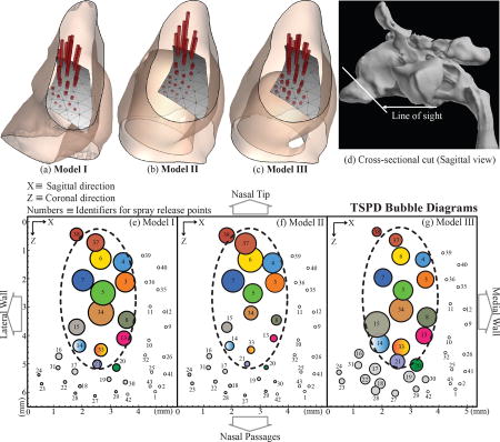
Figure 7 plots the mass fraction of spray particles deposited in the LMS for each of the 27 safe release locations (see §2.3.1 for details on the spray release points and release contour). Based on the numerical identity of the release points (along the horizontal axis in Figure 7), the deposition patterns, in terms of the peak and plateau zones, were congruous for the three test models, with the optimal release points still localized in the same areas of the release contour. In this context, Figures 8(a)–(c) demonstrate an alternate view with the extruded spikes at each release point denoting the quantity of LMS deposits as well as the direction vector of the spray axis. In Figures 8(e)–(g), we projected the release contour on to the XZ plane (parallel to the floor of the hard palate) and traced “bubble-diagrams” where the incrementing circle sizes represent proportionally higher topical deposits at the LMS, with the center of each circle being the projection of the corresponding release point. Note that the color schematic in Figures 8(e)–(g) is such that the same release point has the same color in the three planar projections. A small optimal zone for the best-possible spray release points was identified and it was the same in all the test models. An oval outline (drawn with dashed line), spanning roughly over a 2mm-by-4.5mm contour, was traced to demarcate that zone in the bubble-diagrams. For the nozzle tip to lie within this optimal zone, the spray axis should subtend an angle of ~ 23.25° to 50.66°, with respect to the vertical.

Figure 7.

Bar diagram of the spray mass fractions deposited in the LMS for particles sprayed from the 27 clinically safe release points in the three test models. The numbers on the horizontal axis indicate the corresponding identifiers of the clinically safe spray release locations, based on their assigned nomenclature by Fluent™ and displayed in Figure 4. The bar heights have been proportionally standardized with the peak deposits in all three models being represented by equally tall bars, albeit with change of vertical unit scale to account for the quantitatively unequal peak deposits. Identical numbers in different models correspond to the same release location coordinates in space. The error bars represent the maximum and minimum deposits from the five particle tracking simulation runs implemented for each spray release point. Deposition data for the spray release points located in the lateral and medial halves of the vestibule has been demarcated by the dashed line. The grey bars indicate the release locations for which turbulence simulations were run (findings to be presented later in this manuscript) to compare with the quantity-based ordering of the LMS deposition data from the laminar simulations. Abbreviations: DL ≡ distal lateral, ML ≡ medial lateral, PL ≡ proximal lateral, DM ≡ distal medial, MM ≡ middle medial, PL ≡ proximal medial. Schematics in Figure 4(e) and (d) portray the physical positioning of these zones, obtained from regional segmentation of the spray release surface.

Figure 8.

Panels (a), (b), and (c) show the topical deposition patterns at the LMS in Models I, II, and III respectively. The nasal vestibule is dilated in Models II and III, owing to the placement of the nozzle contour, thereby mimicking nozzle insertion effects in a real nose. The height of the red spike at each release point is proportional to the deposited mass fraction corresponding to that spray release location. The spike heights have been proportionally standardized with the peak deposits in the three test models being represented by equally tall spikes. Direction vectors of the spikes are oriented from the centroid of the nostril to the corresponding release point. The letter “S” marks the septal side of the nasal lining. Panel (d) shows the sectional cut through which the depictions in (a), (b), and (c) were visualized. The “bubble-diagrams” in panels (e), (f), and (g) show an alternate visual representation of the same information. Here the release contour has been projected on the XZ plane, roughly parallel to the floor of the hard palate. The bubble sizes are proportional to the LMS deposit corresponding to the release location whose projection is the center of that bubble. The color scheme was so chosen that the findings for the same release point have the same color, in all three models. Note the unsafe release points were marked by the tiny hollow circles. We identified a small optimal zone for the best-possible spray release points and the oval outline (drawn with the dashed line) roughly demarcated that zone. For scaled representation, its size is compared to the US quarter-dollar coin. Panel (h) presents the bubble diagram-styled LMS deposition results for Model I, with the particle release locations at the respective nozzle tips of the spray bottle contours inserted in Models II and III. Panels (i) and (j) demonstrate the LMS deposits for Models II and III respectively, when the particles are released from the tip of the nozzle inserted in the 3D reconstruction for each. When compared to the main data from panels (e)–(g), bubble diameters in panels (i) and (j) have comparable rank-orders with the same trend as the ones in panel (h). Note: Nozzle Tip 1 ≡ locational coordinate of the nozzle tip as observed for the spray bottle orientation in Model II, Nozzle Tip 2 ≡ locational coordinate of the nozzle tip for the spray bottle orientation in Model III.

For a statistical check of the congruity of TSPD patterns with respect to the release locations, we ran the Spearman’s rank correlation test over three different selections of paired groups (Models I and II, Models I and III, and Models II and III) with respect to the corresponding LMS deposits. For each model, the test ranked the deposits from the different release points according to their magnitudes and then assessed how well these rank-orders correlate between two different models. For the comparison between Models I and II, the test returned R = 0.929, with the two-tailed p < 0.000001. For Models I and III, we had R = 0.866, with the two-tailed p < 0.000001. For Models II and III, the test gave R = 0.767, with the two-tailed p < 0.000003. Thus, the congruity of deposition patterns across the three test models could be considered statistically significant.

The same grid of spray release locations (as shown in Figure 4) and spray directions (from the nostril centroid to the corresponding release point) were used in all three models for a standardized comparison. To complement the main results, we extracted the locational coordinates of the inserted nozzle tips in the two derived models. We named them as “Nozzle Tip 1” and “Nozzle Tip 2” for the respective spray bottle orientations in Models II and III. Subsequently, four distinct spray axis directions A, B, C, D were calculated: (A and B) from the centroid of left nostril plane in Model I to Nozzle Tip 1 and Nozzle Tip 2, (C) from the centroid of the nozzle base in Model II to Nozzle Tip 1, and (D) from the centroid of nozzle base in Model III to Nozzle Tip 2. We implemented particle simulations in Model I for the spray axis parameters A, B; in Model II for the spray axis parameters C, and in Model III for the spray axis parameters D. Figures 8(h)–(j) show the bubble diagrams for the corresponding LMS topical deposits in Models I, II, III respectively. The rank-order for the TSPDs, when compared to the larger data-set from Figures 8(e)–(g), revealed the same directional trend in Model I, as in Model II and Model III. Thus, even with exact spray release points for the corresponding nozzle in the derived models, the relative TSPD patterns were found to be congruous between the test cases. This lends support to the reliability of the overall study design where TSPDs were obtained for a grid of release locations for a single nozzle orientation (one each in Models II and III). Finally, note that the plotted bubble-diagrams in Figures 8(h)–(j) also included the outline of the optimal oval-shaped zone from Figures 8(e)–(g), to compare the location of the nozzle tips in Models II and III with respect to the potentially more efficient spray release points.

3.2.1. Comparing the airflow patterns in the models

Presence of the nozzle contour in the anterior vestibule altered the airflow patterns in the anterior segments of the nasal duct in Models II and III, in comparison to the flow patterns in base Model I. However, owing to the high initial speed (19.2 m/s) of the sprayed particles, these fluctuating trends in the anterior vestibule were initially superseded by the inertial motion of the particles. In Figure 9, we separately tracked the motion of one representative 5 µm particle and another 25 µm particle, sprayed from release location 5 at 45° to the Y and Z axes, and 90° to the X axis. Along the particle trajectories, the tiny red circle marked the location where the inertial motion of the particle, contributed by its initial exit speed, ceased. The particle deceleration was primarily induced by the ambient air drag and gravity. Following the cessation of the inertial motion, the particle fell vertically under gravity, in the absence of an ambient airflow. See panels (a), (c), (e) for the 5 µm particle and (g), (i), (k) for the 25 µm particle, for such no-flow considerations. On the contrary, the inspiratory airflow in panels (b), (d), (f) for the 5 µm particle and (h), (j), (l) for the 25 µm particle dominated the particle dynamics following the cessation of its initial inertial motion, and transported the particle to the pharyngeal outlet (for the representative 5 µm particle) and to the ethmoids (for the representative 25 µm particle), via convoluted flow streamline paths. As a corollary, the observations suggested the increasing precedence of the inspired airflow on the sprayed particle motion as the particle traversed deeper into the nasal cavity, with the lighter particles being affected early while still in the anterior vestibule.

Figure 9.

Sample trajectories (colored black) of one representative 5-µm-sized particle and one representative 25-µm-sized particle in the three models, without any ambient airflow, namely in panels (a), (c), (e) and (g) (i), (k), and with inspiratory airflow passing through the models, namely in panels (b), (d), (f) and (h), (j), (k). The tiny red circles mark the locations where the inertial motion, contributed by the spray exit velocity, ceases (with deceleration primarily induced by the air drag and gravity), following which the particles either fall freely under gravity (downward acceleration g) in the no-airflow simulations or are transported via the convoluted paths of the fluid streamlines in the simulations with ambient airflow. Heavier particles penetrate deeper before the cessation of the inertial motion. In the presence of inspiratory airflow, the representative 5 µm particle escapes through the pharyngeal outlet, while the representative 25 µm particle gets deposited in the ethmoid sinus. The representative particles were all sprayed with an exit speed of 19.2 m/s from release location 5. Initial direction of the particles subtended 45° with both Y and Z axes, and was at 90° to the X axis.

Figure 10 tracks the airflow velocity contour maps on six different cross-sections (namely, c/s-1 to c/s-6) in the nasal models. The disturbances in the anterior vestibule manifested in sections c/s-1 and c/s-2. The presence of the spray bottle contour created stagnation zones with low flow speeds in the regions posteriorly proximal to the nozzle tip. See the c/s-1 sections in Models II and III for the corresponding flow profiles, with the black circles apprximately delineating the stagnation zones. Also note that the cross-sectional areas in c/s-1 in Models II and III were quite different than in Model I, owing to the anterior vestibule being dilated by the nozzle insertion. Relative differences between the nasal airflows gradually evened out as we probed deeper into the airways, with the flow patterns showing trends of homogeneity in the vestibular cavity (c/s-3) anterior to the meatal region. Posterior to the turbinates, the ambient airflow dominated the inertial motion of all the sprayed particle sizes that went into the LMS (see representative examples in Figure 9). For section c/s-4, spanning across through the antrostomy window (which is the opening to the maxillary sinus in the post-operative anatomy), the airflow trends in the different models were very similar. Consequently, the inspired airflow exerted comparable effects on the sprayed particles in the proximity of the ostiomeatal complex and contributed towards similar spray release locations generating larger maxillary deposits in all three models.

Figure 10.

Color maps of the velocity magnitude of the inspired airflow field across six different cross-sections (c/s-1 to c/s-6). See the top-most panel for the cross-sections selected. Left-right orientation of the graphics in each of the flow profile panels respectively corresponds to the left and right sides of the study subject. The flow patterns observed on c/s-1 noticeably demonstrate the fluctuations from nozzle placement (in Models II and III) in the anterior vestibule. Stagnation zones closely posterior to the nozzle tips are demarcated by the black circles. Flow profiles display increasing conformity at larger penetration depths.

3.2.2. On different TSPD quantities in the test models

There was a caveat in terms of the absolute quantities of topical deposition in the LMS. As can be seen from Figure 7, the peak deposit in Model I was more than five times the peak deposit in Model II. However, Model I and Model III presented somewhat similar peak deposits. To explain, we analyzed the spray deposits in the different regions of the nasal model for a representative simulation, with the particles ejected from release point 5 (see Figure 4(f)) corresponding to a spray axis angle of 34.95° to the vertical, the axis being directed from the left nostril centroid to the release point. While the anterior deposits were exactly same in all three models and with the deposits in the other regions (except the left maxillary sinus) being comparable in order, the biggest differential arose from the larger sprayed mass escaping the pharyngeal outlet in Model II. For an initial shot weight of 100 mg, the spray mass that escaped through the outlet were: 0.0634 mg in Model I, 0.0828 mg in Model II, and 0.0660 mg in Model III. This contributed to the quantitatively less particle transport to the Model II LMS. Particle sizes depositing in the LMS of Model I ranged from 5–40 µm, for Model III they ranged from 5–30 µm, while for Model II, the particles settling on the maxillary sinus belonged to the 10–25 µm size range. This may be explained in terms of the dissimilar effects exerted by the ambient airflow (with fluctuating patterns in the anterior vestibule owing to the nozzle insertion) on the lighter particles in the anterior segment of the nasal cavity. For a visual example, see Figures 9(a)–(f), where for the lighter 5 µm particle motion, the airflow gained precedence when the particle was still very close to c/s-1.

3.2.3. On the sensitivity of the modeling framework

The congruity between the three models could be arguably ascribed to the insensitivity of the computational modeling algorithms. To check, we perturbed the simulation conditions and did the flow tracking in the three models through the shear-stress transport (SST) based k-ω turbulence model, with low Re correction. Inspired airflow rates and the inlet-outlet pressure gradients were respectively 19.78 Liters/min and −7.81 Pa in Model I, 19.68 Liters/min and −9.15 Pa in Model II, and 19.68 Liters/min and −9.60 Pa in Model III.

For a representative check of the particle deposition trends, we simulated the sprayed drug delivery from the three release locations 7, 21, and 3 (see Figure 4(e) and (f) for their respective locations). The TSPDs followed the same trend (Figure 11), with LMS deposit for release location 7 > LMS deposit for release point 3 > LMS deposit for release point 21, as was previously observed in Figure 7 obtained from laminar-viscous flow modeling in the three models. The consistent rank-order corroborates the robustness of our modeling framework and insists that the TSPD congruity between Models I, II, and III cannot be ascribed to any methods-related insensitivity.

Figure 11.

Representative spray deposit fractions in the LMS, based on inspiratory airflow modeled using k-ω turbulence framework. The relative order of the TSPDs matched with the results presented earlier in Figure 7 obtained from laminar simulations.

3.3. Variability of the numerical results for spray deposition

The laminar spray simulations were run 5 times for each release point, in each of the Models I, II, and III. Power analyses were performed to determine the power of correctly detecting that our sample mean deposition mass fraction in each model based on 5 simulation runs would lie within a pre-determined desired precision of the true population mean deposition mass fraction. The following desired precision (error margin) between our sample mean deposition mass fraction and the true population mean deposition mass fraction for our three models were specified: (1) error margin of 0.00045 for Model I; (2) error margin of 0.00009 for Model II; and (3) error margin of 0.00047 for Model III. For example, in Model I, we calculated the power such that the difference between our sample mean deposition mass fraction and the true population mean deposition mass fraction is within 0.00045. In each model, we chose the error margin to be 5% of the peak mass deposition fraction in the LMS. At 5% level of significance we obtained a 98% mean power for Model I, a 93% mean power for Model II, and a 96% power for Model III. See Figure 12 for a depiction of the representative power curves for the three test models corresponding to release point 1. Implementation of power analysis in the present work was identical to the approach used earlier.³⁵

Figure 12.

Graphical representation of the power of the sample with respect to the sample size. The latter, in this case, is the number of numerical runs implemented for particle tracking corresponding to each release point. These representative power curves were traced out for the release location 1 in all the three test models.

4. DISCUSSION

We explored methodological ambiguities related to the inclusion of a spray bottle inside the anterior nasal vestibule of a 3D computational reconstruction, in the context of numerically ascertaining the optimal spray release locations for improved topical drug delivery. Three test models were developed: one base model without nozzle subtraction (Model I) and two additional derived models (Models II, III) with two very different orientations of subtracted nozzle from the nasal airspace (along with laterally dilated anterior vestibule to account for nozzle insertion), developed from the post-surgical CT scans of the same subject with a history of CRS. We performed inspiratory airflow simulations under steady state conditions in these three test models. Sprayed particle transport was then numerically tracked for a lattice of 27 clinically safe nasal spray release points and directions. The optimal zone for spray release for better drug penetration to the maxillary sinus (a crucial target site for treating CRS) stayed the same in all three models. The flow features were such that they could be reliably modeled within a laminar framework. See Figure 8 for the optimal spray release zone, which revealed to be rather tiny and covered a roughly 2mm-by-4.5mm oval contour in all three test models. The results thus indicate a redundancy of nozzle insertion (i.e. subtracting the nozzle contour from the nasal vestibule) for such 3D anatomic reconstructions.

There can, however, be several points of critique connected to the study design and assumptions, as examined hereunder:

• Excerpts from the user instructions for Fluticasone nasal spray state:³⁶ “Start to breathe in through your nose, and while breathing in press firmly and quickly down 1 time on the applicator to release the spray… Breathe in gently through the nostril.” To conform to the first instruction, we did not allow any time lag between the inspiratory airflow cycle and the sprayed particle release in the simulations. We interpreted the instruction to “breathe in gently” as a preliminary justification for modeling the airflow under steady state conditions. However, alternate instructions available online³⁷ at times do recommend “sniffing” while applying nasal sprays.

  Addressing the ambiguity warranted a careful consideration of the breathing rates for the test subject. While we did not have sniffing measurements for this specific patient, another subject (a 28-year-old Caucasian male weighing 92 kg with height 70.81 inches) with a similar metabolic rate (BMI 28.4, in comparison to 28.3 for the current test subject) was identified from a cohort of CRS patients, for whom we have been collecting pre-surgery breathing data with IRB approval at the University of North Carolina at Chapel Hill. The measurements were recorded using a portable respiratory inductive plethysmograph (LifeShirt®, VivoMetric, San Diego, CA) that tracks breathing through chest-volume expansion-relaxation trends. For the pre-surgery diseased subject, the normal inspiratory flow rate was 13.18 Liters/min and the sniffing rate was 13.62 Liters/min. As stated in §2.4.2, assuming identical allometrically scaled breathing rates for post-operative CRS subjects and non-symptomatic healthy population, the regular breathing would improve to ~20.13 Liters/min post surgical intervention. The factor of improvement was approximately 1.53, and multiplying the pre-surgery sniffing by the same factor, the prediction for post-surgery sniffing rate approximated to 20.84 Liters/min. Laminar steady (or quasi-steady) flow has been shown to be a reasonable assumption^{26, 38} for such airflow rates.

  Recent time-dependent computations^{39, 40} have yielded results in agreement with the steady state framework assumed for resting breathing. Nonetheless, steady state inspiration, while purportedly a good approximation for the brief single-cycle respiratory span during which the sprayed particles are assumed to propagate through the sinonasal cavity, is still an idealization. Inspiration and expiration demonstrably have some acceleratory and deceleratory components. To reliably assess time-variable effects like nasal valve region collapse or constriction that happens during sniffing, more realistic simulations will require completely unsteady flow tracking.

• The three models differed only in the anterior portion (refer back to Figure 2) of the left nasal airspace. Model I was built from the subject-specific CT scans, while Models II and III had the anterior portions built from scans of a 3D printed model (of Model I) with a spray nozzle inserted at the left nostril. To compare between the models, care was taken that apart from this nozzle placement zone, the computational subject-specific reconstructions stayed analogous and comparable. However, it should be noted that the subtle geometrical effects of the nozzle placement on the nasal lining may extend beyond this anterior chunk, based on subject-specific variations in tissue pliability.

• Topical deposits at the (left) maxillary sinus were miniscule and less than 1% spray mass fraction. The comprehensive TSPD patterns also differed subtly between the three test models (for details, see §3.2). Such variations between numerical models with and without the spray nozzle are in agreement with published results.⁸ However, the core aim of our study was to explore if nozzle subtraction and vestibular dilation were essential to identify the release points which would allow for the best possible sinonasal target site deposition. Thus, the absolute quantities of deposits were not of any compelling relevance and we focused more on the pattern of targeted deposition with respect to the lattice of spray release locations.

• While quantifying the drug transport to the target sinonasal sites (in this study, the LMS), we have assumed that the sprayed particles get trapped on the internal cavity walls (mimicking the tissue surfaces), without any further mucus drainage transport or escape probabilities. This is an idealized assumption, and it would be interesting to capture the nuances beyond the scope of these current limitations. Nasal mucus is essentially non-Newtonian in terms of its fluidic properties and this makes modeling its viscosity challenging.⁴¹ In this context, the reader may refer to a recent CFD-based study⁹ investigating the effects of mucociliary clearance on drug uptake in the human nasal cavity (excluding the paranasal sinuses). Also see the study by Wooton and Ku⁴² for a particularly interesting account (albeit not for respiratory flows) on the complex fluid dynamical subtleties associated with other classes of biological flows.

• We assumed that the particles in motion never had any kinematic interactions with the other sprayed particles during their sinonasal transport. Nor was there any effect of the particle’s motion on the ambient inspiratory airflow. Additionally, their material density, sizes, and spherical shapes were considered to remain unchanged as they propagated through the nasal cavity.

Despite the aforementioned caveats, this methods study, to summarize, does make the important suggestion that vestibular nozzle insertion in a 3D nasal model is not essential for reliable airflow simulations, particularly while identifying the optimal release conditions for targeted delivery of sprayed intranasal drugs. The inference alleviates the process of reconstructing anatomically realistic sinonasal models from patient-specific CT imaging. The findings will provide an important functional tool towards using 3D computational modeling on large cohorts of patient scans, which can help in recommending new usage instructions for aerosolized sprays aimed at maximizing particulate transport and deposition at the nasal target sites, hence providing a more effective therapeutic care for diseases like chronic rhinosinusitis.

Table II.

Mean mass fraction deposits at the left maxillary sinus, based on 5 simulation runs for each release location in each test model, along with the corresponding standard deviations. Left-most column indicates the spray release point identifiers.

Rel. Pt.	Model I		Model II		Model III
	Mass fraction %	Standard deviation	Mass fraction %	Standard deviation	Mass fraction %	Standard deviation
3	0.00529	0.000127279	0.0009984	0.0000294669	0.003818	0.000216032
4	0.004678	0.000176833	0.001082	0.0000363318	0.00288	0.000112472
5	0.008526	0.000140285	0.0009966	0.0000875717	0.005278	0.0000834865
6	0.006098	0.000110995	0.001812	0.000107564	0.004156	0.0000988939
7	0.006236	0.0000328634	0.001392	0.0000641872	0.004344	0.0000867756
8	0.003834	0.000281034	0.000224	0.0000260096	0.005174	0.000127201
13	0.00266	0.000162635	0.0000861	0.0000190164	0.003658	0.000127554
14	0.001896	0.0000673053	0.0001612	0.0000119038	0.00496	0.000293002
15	0.003342	0.000127945	0.0002386	0.0000203052	0.009408	0.000335738
16	0.000357	0.0000175642	0.0000379	0.00000257196	0.000831	0.0000677237
17	0.0002654	0.0000656415	0.0000236	0.00000651038	0.00153	0.000121037
18	0.00002524	0.0000133129	0.000007196	0.00000193154	0.001154	0.0000947629
19	0.00010984	0.0000362876	0.00000783	0.00000432576	0.001432	0.0000952365
20	0.0005118	0.0000802322	0.000016644	0.00000599314	0.001952	0.00014025
21	0.0007564	0.0000371053	0.000037	0.00000955693	0.002732	0.0000960208
22	0.000027158	0.0000131633	0.000008688	0.00000149655	0.0010216	0.0000763891
23	0	–	0.00000485	0.00000397665	0.0002336	0.0000124218
24	0	–	0.000007704	0.0000031044	0.0001592	0.0000117558
27	0	–	0	–	0.0004008	0.0000281727
28	0	–	0.00000183152	0.0000013478	0.0007478	0.0000187003
29	0	–	0	–	0.0002794	0.0000307782
30	0.0001037	0.0000289418	0	–	0.0003976	0.0000254224
31	0.00007694	0.0000139414	0.00001854	0.00000485829	0.0004614	0.0000478571
33	0.001952	0.0000903881	0.00009594	0.0000158248	0.003846	0.000199324
34	0.009186	0.000258225	0.0004806	0.00000585662	0.00803	0.000433359
37	0.004022	0.0000491935	0.001252	0.0000334664	0.002088	0.0000593296
38	0.002024	0.0000522494	0.0006216	0.0000299717	0.000858	0.0000256515

References

- 1.Fokkens WJ, Lund VJ, Mullol J, Bachert C, Alobid I, Baroody F, Cohen N, Cervin A, Douglas R, Gevaert P, et al. European position paper on rhinosinusitis and nasal polyps 2012. Rhinology. Supplement. 2012;(23):3. [PubMed] [Google Scholar]
- 2.Benninger MS, Ferguson BJ, Hadley JA, Hamilos DL, Jacobs M, Kennedy DW, Lanza DC, Marple BF, Osguthorpe JD, Stankiewicz JA, et al. Adult chronic rhinosinusitis: definitions, diagnosis, epidemiology, and pathophysiology. Otolaryngology-Head and Neck Surgery. 2003;129(3):S1–S32. doi: 10.1016/s0194-5998(03)01397-4. [DOI] [PubMed] [Google Scholar]
- 3.Rosenfeld RM, Andes D, Bhattacharyya N, Cheung D, Eisenberg S, Ganiats TG, Gelzer A, Hamilos D, Haydon RC, Hudgins PA, et al. Clinical practice guideline: adult sinusitis. Otolaryngology-Head and Neck Surgery. 2007;137(3):S1–S31. doi: 10.1016/j.otohns.2007.06.726. [DOI] [PubMed] [Google Scholar]
- 4.Albu S, Baciut M. Failures in endoscopic surgery of the maxillary sinus. Otolaryngology—Head and Neck Surgery. 2010;142(2):196–201. doi: 10.1016/j.otohns.2009.10.038. [DOI] [PubMed] [Google Scholar]
- 5.Frank DO, Kimbell JS, Pawar S, Rhee JS. Effects of anatomy and particle size on nasal sprays and nebulizers. Otolaryngology–Head and Neck Surgery. 2012;146(2):313–319. doi: 10.1177/0194599811427519. [DOI] [PMC free article] [PubMed] [Google Scholar]
- 6.Kimbell JS, Segal RA, Asgharian B, Wong BA, Schroeter JD, Southall JP, Dickens CJ, Brace G, Miller FJ. Characterization of deposition from nasal spray devices using a computational fluid dynamics model of the human nasal passages. Journal of aerosol medicine. 2007;20(1):59–74. doi: 10.1089/jam.2006.0531. [DOI] [PubMed] [Google Scholar]
- 7.Shi H, Kleinstreuer C, Zhang Z. Laminar airflow and nanoparticle or vapor deposition in a human nasal cavity model. Journal of biomechanical engineering. 2006;128(5):697–706. doi: 10.1115/1.2244574. [DOI] [PubMed] [Google Scholar]
- 8.Inthavong K, Ge Q, Se CM, Yang W, Tu J. Simulation of sprayed particle deposition in a human nasal cavity including a nasal spray device. Journal of Aerosol Science. 2011;42(2):100–113. [Google Scholar]
- 9.Rygg A, Longest PW. Absorption and clearance of pharmaceutical aerosols in the human nose: development of a CFD model. Journal of aerosol medicine and pulmonary drug delivery. 2016;29(5):416–431. doi: 10.1089/jamp.2015.1252. [DOI] [PMC free article] [PubMed] [Google Scholar]
- 10.Kimbell J, Stricklin D, Schroeter J. Simulating nasal spray deposition: effects of spray nozzle presence in the nasal vestibule. Journal of aerosol medicine and pulmonary drug delivery. 2015;28(3):A-41. [Google Scholar]
- 11.Benninger MS, Hadley JA, Osguthorpe JD, Marple BF, Leopold DA, Derebery MJ, Hannley M. Techniques of intranasal steroid use. Otolaryngology-Head and Neck Surgery. 2004;130(1):5–24. doi: 10.1016/S0194-5998(03)02085-0. [DOI] [PubMed] [Google Scholar]
- 12.Xi J, Longest PW. Numerical predictions of submicrometer aerosol deposition in the nasal cavity using a novel drift flux approach. International Journal of Heat and Mass Transfer. 2008;51(23):5562–5577. [Google Scholar]
- 13.Shanley KT, Zamankhan P, Ahmadi G, Hopke PK, Cheng YS. Numerical simulations investigating the regional and overall deposition efficiency of the human nasal cavity. Inhalation toxicology. 2008;20(12):1093–1100. doi: 10.1080/08958370802130379. [DOI] [PubMed] [Google Scholar]
- 14.Kelly J, Prasad A, Wexler AS. Detailed flow patterns in the nasal cavity. Journal of Applied Physiology. 2000;89(1):323–337. doi: 10.1152/jappl.2000.89.1.323. [DOI] [PubMed] [Google Scholar]
- 15.Basu S, Kimbell JS, Zanation AM, Ebert CS, Senior BA. Clinical questions and the role CFD can play. Bulletin of the American Physical Society. 2016;61 [Google Scholar]
- 16.Frank-Ito D, Senior B, Zanation A, Ebert C, Kimbell J. Investigating optimal head position for topical drug administration in chronic rhinosinusitis patientsl. Respiratory Drug Delivery 2016. 2016;2:303–308. [Google Scholar]
- 17.AT Borojeni A, Frank-Ito DO, Kimbell JS, Rhee JS, Garcia GJ. Creation of an idealized nasopharynx geometry for accurate computational fluid dynamics simulations of nasal airflow in patient-specific models lacking the nasopharynx anatomy. International Journal for Numerical Methods in Biomedical Engineering. 2017;33(5) doi: 10.1002/cnm.2825. e2825–n/a, E2825 CNM-Jan-16-0004.R1. [DOI] [PMC free article] [PubMed] [Google Scholar]
- 18.Frank-Ito DO, Wofford M, Schroeter JD, Kimbell JS. Influence of mesh density on airflow and particle deposition in sinonasal airway modeling. Journal of aerosol medicine and pulmonary drug delivery. 2016;29(1):46–56. doi: 10.1089/jamp.2014.1188. [DOI] [PMC free article] [PubMed] [Google Scholar]
- 19.Basu S, Witten N, Kimbell J. Influence of localized mesh refinement on numerical simulations of post-surgical sinonasal airflow. Journal of aerosol medicine and pulmonary drug delivery. 2017;30(3):A-14. [Google Scholar]
- 20.Finlay WH. The Mechanics of Inhaled Pharmaceutical Aerosols: An Introduction. Academic Press; 2001. [Google Scholar]
- 21.Liu X, Doub WH, Guo C. Assessment of the influence factors on nasal spray droplet velocity using phase-doppler anemometry (pda) AAPS Pharmscitech. 2011;12(1):337–343. doi: 10.1208/s12249-011-9594-1. [DOI] [PMC free article] [PubMed] [Google Scholar]
- 22.Garcia GJ, Schroeter JD, Segal RA, Stanek J, Foureman GL, Kimbell JS. Dosimetry of nasal uptake of water-soluble and reactive gases: a first study of interhuman variability. Inhalation toxicology. 2009;21(7):607–618. doi: 10.1080/08958370802320186. [DOI] [PubMed] [Google Scholar]
- 23.ANSYS Fluent Theory Guide version 14.5. Vol. 275 ANSYS Inc, Southpointe; [Google Scholar]
- 24.Morsi S, Alexander A. An investigation of particle trajectories in two-phase flow systems. Journal of Fluid Mechanics. 1972;55(2):193–208. [Google Scholar]
- 25.Schroeter JD, Tewksbury EW, Wong BA, Kimbell JS. Experimental measurements and computational predictions of regional particle deposition in a sectional nasal model. Journal of aerosol medicine and pulmonary drug delivery. 2015;28(1):20–29. doi: 10.1089/jamp.2013.1084. [DOI] [PubMed] [Google Scholar]
- 26.Shi H, Kleinstreuer C, Zhang Z. Dilute suspension flow with nanoparticle deposition in a representative nasal airway model. Physics of Fluids. 2008;20(1) 013 301. [Google Scholar]
- 27.White FM. Fluid Mechanics. 5. Boston: McGraw-Hill Book Company; 2003. [Google Scholar]
- 28.Wygnanski I, Champagne F. On transition in a pipe. part 1. the origin of puffs and slugs and the flow in a turbulent slug. Journal of Fluid Mechanics. 1973;59(02):281–335. [Google Scholar]
- 29.Darbyshire A, Mullin T. Transition to turbulence in constant-mass-flux pipe flow. Journal of Fluid Mechanics. 1995;289:83–114. [Google Scholar]
- 30.Stremler MA, Salmanzadeh A, Basu S, Williamson CH. A mathematical model of 2P and 2C vortex wakes. Journal of Fluids and Structures. 2011;27(5):774–783. [Google Scholar]
- 31.Basu S. Ph.D.thesis. Virginia Polytechnic Institute and State University; 2014. Dynamics of vortices in complex wakes: modeling, analysis, and experiments; p. 131. [Google Scholar]
- 32.Stremler MA, Basu S. On point vortex models of exotic bluff body wakes. Fluid Dynamics Research. 2014;46(6) 061 410. [Google Scholar]
- 33.Basu S, Stremler MA. On the motion of two point vortex pairs with glide-reflective symmetry in a periodic strip. Physics of Fluids. 2015;27(10) 103 603. [Google Scholar]
- 34.Basu S, Stremler MA. Exploring the dynamics of ’2P’ wakes with reflective symmetry using point vortices. Journal of Fluid Mechanics. 2017 doi: 10.1017/jfm.2017.563. [DOI] [Google Scholar]
- 35.Frank DO, Kimbell JS, Cannon D, Pawar SS, Rhee JS. Deviated nasal septum hinders intranasal sprays: a computer simulation study. Rhinology. 2012;50(3):311. doi: 10.4193/Rhin. [DOI] [PMC free article] [PubMed] [Google Scholar]
- 36.Fluticasone nasal spray - FDA prescribing information, side effects and uses. 2017 URL https://www.drugs.com/pro/fluticasone-nasal-spray.html.
- 37.Healthline instructions for nasal spray use. 2017 URL https://www.healthline.com/health/general-use/how-to-use-nasal-spray#introduction1.
- 38.Zhao K, Dalton P, Yang GC, Scherer PW. Numerical modeling of turbulent and laminar airflow and odorant transport during sniffing in the human and rat nose. Chemical senses. 2005;31(2):107–118. doi: 10.1093/chemse/bjj008. [DOI] [PubMed] [Google Scholar]
- 39.Chen XB, Lee HP, Chong VFH, Wang DY. Aerodynamic characteristics inside the rhino-sinonasal cavity after functional endoscopic sinus surgery. American journal of rhinology & allergy. 2011;25(6):388–392. doi: 10.2500/ajra.2011.25.3669. [DOI] [PubMed] [Google Scholar]
- 40.Bahmanzadeh H, Abouali O, Ahmadi G. Unsteady particle tracking of micro-particle deposition in the human nasal cavity under cyclic inspiratory flow. Journal of Aerosol Science. 2016;101:86–103. [Google Scholar]
- 41.Quraishi M, Jones N, Mason J. The rheology of nasal mucus: a review. Clinical Otolaryngology & Allied Sciences. 1998;23(5):403–413. doi: 10.1046/j.1365-2273.1998.00172.x. [DOI] [PubMed] [Google Scholar]
- 42.Wootton DM, Ku DN. Fluid mechanics of vascular systems, diseases, and thrombosis. Annual review of biomedical engineering. 1999;1(1):299–329. doi: 10.1146/annurev.bioeng.1.1.299. [DOI] [PubMed] [Google Scholar]