A two-stage model for wearable device data

Summary

Recent advances of wearable computing technology have allowed continuous health monitoring in large observational studies and clinical trials. Examples of data collected by wearable devices include minute-by-minute physical activity proxies measured by accelerometers or heart rate. The analysis of data generated by wearable devices has so far been quite limited to crude summaries, for example, the mean activity count over the day. To better utilize the full data and account for the dynamics of activity level in the time domain, we introduce a two-stage regression model for the minute-by-minute physical activity proxy data. The model allows for both time-varying parameters and time-invariant parameters, which helps capture both the transition dynamics between active/inactive periods (Stage 1) and the activity intensity dynamics during active periods (Stage 2). The approach extends methods developed for zero-inflated Poisson data to account for the high-dimensionality and time-dependence of the high density data generated by wearable devices. Methods are motivated by and applied to the Baltimore Longitudinal Study of Aging.

1. Background

Recent advances of wearable computing technology have allowed continuous health monitoring in large observational studies and clinical trials. Activity trackers and heart rate monitors are two such devices that are widely used. Activity trackers are used to objectively measure the level and timing of physical activities. They have been used in many scientific studies to supplement or even replace self-reported questionnaires that can be subject to large measurement error and uncontrollable biases (Neilson et al., 2008). Two comprehensive reviews of such studies were provided by (John and Freedson, 2012) and (Yang and Hsu, 2010). Heart rate monitors have an even longer history in health studies (see (Terbizan et al., 2002)), because heart rate is directly related to the physiology of human body and is used extensively to study energy expenditure.

Actiheart (Cambridge Neurotechnology Ltd, Papworth, UK) was one of the earliest wearable devices that combined heart rate and motion sensing (Brage et al., 2005). Other integrated multi-sensor trackers have become widely available over the past 5 years both in research and the consumer market (Bai et al., 2016). Wearable device data are sampled at a constant rate set by the manufacturer or user. Modern accelerometers can provide densely sampled tri-axial raw accelerometry data, or uni-axial summaries of activity level within various epochs. The raw accelerometry data consist of 3 time series corresponding to the sensor’s instantaneous acceleration along 3 orthogonal directions, commonly with 10–100 samples per second on each axis. The raw accelerometry data provide high resolution information on the changes of acceleration, and are standard measurements in modern accelerometry studies. Another type of data is the uni-axial summary data in epochs (in second, minute, etc.), which summarizes information about the intensity of activity from the raw data. Commonly used summary data include various versions of activity count, which are provided by the accelerometer manufacturer, and open-source metrics such as the Activity Index (Bai et al., 2016) and Mean Amplitude Deviation (Vähä-Ypyä et al., 2015). This reduced format of data is often preferred in large epidemiological studies, as the size and complexity of the data are reduced while the resulting summaries are considered to be informative enough to describe the overall trajectory of physical activity.

In this paper we will focus on the summary data aggregated at the minute level, which results in 1440 observations per day or more than 10000 per week. The data structure is of the type Y_ij(t), where i(= 1, 2, …, n) denotes subject, j(= 1, 2, …, J_i) denotes the day and t(= 1, 2, …, T_ij) denotes the time of day. The measurement, Y_ij(t), is usually a non-negative number with various interpretations, depending on the application. For activity trackers, Y_ij(t) is the activity counts or number of steps, which are used as proxies of the activity intensity.

Although such data have been collected in many public health and medical studies, models and analyses are limited to crude summaries, such as the total activity count over a 24-hour period. Despite concerns about the loss of information during the summarization process, only a few analyses utilized the full data. Schrack et al. (2014); Goldsmith et al. (2015); Xiao et al. (2015) have investigated the association between minute-by-minute activity counts and health covariates, via various methods including functional regression and bivariate smoothing. Li et al. (2014, 2015) studied the dynamics of 5-minute energy expenditure level (estimated by accelerometers) using functional principal component analysis and penalized splines. Shou et al. (2015) analyzed activity data using principal component analysis to extract the main patterns of variation in activity data. Our goal is to provide a new and systematic methodology to assess the effects of covariates on both the incidence rate and level of physical activity. Although our motivating data are minute-by-minute activity counts (AC), the proposed model can easily be used in other applications where data are densely sampled curves and the outcome is a mixture between a point mass at zero and a continuous positive distribution.

In Section 2, we introduce a two-stage regression model for the transition between active/inactive periods (stage 1) and activity intensity during active periods (stage 2). In Section 3, we describe the estimation method and provide the asymptotic properties of the estimators. A simulation study is presented in Section 4 to demonstrate the performance of the estimation. Methods are applied in Section 5 to the Baltimore Longitudinal Study of Aging (BLSA) to quantify the effect of age, gender and body mass index (BMI) on daily activity trajectories. The paper will conclude with a discussion in Section 6.

2. Two-stage Model

2.1 Notation

We consider the case when the data are collected from a group of subjects (i = 1, 2, …, n) during one day (J_i = 1) for a fixed number of time units (T_ij = T). Assume the measurement Y(t) is observed at every time point t = 1, …, T. We define the time-dependent binary process A(t), which is an event indicator (e.g. whether the subject was active) at time t. This can be obtained through direct observation or by thresholding Y(t); for example, A(t) = 1 if and only if Y(t) > 0. If v is the counting measure on {1, 2, …, T} then the total number of events can be written as ${\displaystyle {\int }_0^{T}A\left(u\right)d\nu \left(u\right)}$, and the total volume of activity proxy from [0, T] is ${\displaystyle {\int }_0^{T}Y\left(u\right)A\left(u\right)d\nu \left(u\right)}$.

Let X(t) denote the vector of covariates, which can include both time-dependent factors, such as the day time indicator or the average of Y(t) in a past window, and time-independent factors such as baseline age, gender. We assume that the observed data {A_i(t), Y_i(t), X_i(t); t = 1, …, T, i = 1, …, n} are i.i.d. replicates of {A(t), Y(t), X(t); t = 1, …, T}, where i is the subject index.

2.2 Model framework

Even though wearable computing data are measured over multiple days, in this paper we will focus on modeling one day of data per subject. This simplifies the modeling strategy by avoiding the between-day correlation of physical activity within-subject. In the data analysis of this paper, we selected one day of data for each subject with the highest total activity count. This can also be achieved by calculating the minute-specific median or mean activity count over multiple activity days. Our analysis indicated that the result did not change significantly with the choice of data reduction. In future studies we plan to address the problem of having multiple days of data per subject. Figure 1 illustrates our conceptual model in the context of activity tracking. For simplicity we only show a six-minute segment of the data. The top panel contains AC, Y_i(t), with no activity (AC= 0) at minutes 1, 2, and 5. The middle panel contains A_i(t), the process indicating whether AC is greater than 0 at time t. For example, when t = 3, 4 or 6, A_i(t) = 1 and ${\displaystyle {\int }_0^t{A}_i\left(u\right)d\nu \left(u\right)}$ increases by 1, indicating the subject was active during that particular time interval. Thus A_i(t) = I{Y_i(t) > 0}, where I{·} is the indicator function. We are interested in quantifying the association between the covariates X_i(t) and the processes A_i(t) and Y_i(t). We further separate X_i(t) into two groups of covariates Z_i(t) and H_i(t), which correspond to covariates with time-invariant effects (which do not vary by time) and covariates with time-varying effects. Separating Z_i(t) and H_i(t) is necessary because the interpretation of their effects is rather different.

Figure 1.

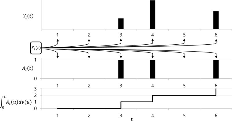
Illustration of conceptual model structure. Outcome Y_i(t) is the activity intensity data, observed only at minute t = 3,4,6 when A_i(t) = 1. ${\displaystyle {\int }_0^t{A}_i\left(u\right)d\nu \left(u\right)}$ is the total active time up to time t. X_i(t) are covariates which affect both Y_i(t) and A_i(t).

In our setting, A_i(t) is observed at every time point t ∈ {1,2, …, T} and T is relatively large (e.g., T = 1440 for one-day of data sampled at the minute level). The notation and structure of the data are similar to those used for continuous marked processes (Pinsky and Karlin, 2010). However, the modeling strategies we use here are different, because wearable computing data are very large and discretized. Our data could also be analyzed using a standard zero-inflated Poisson count model, but such an approach would be quite involved and relatively hard to implement. Therefore, we choose to present an alternative approach, a two-stage model.

2.3 Model specification

To assess the effect of covariates X_i(t) on A_i(t) and Y_i(t), we first separate X_i(t) into Z_i(t) and H_i(t) by formally defining X_i(t) = {1, Z_i(t)^⊤, H_i(t)^⊤}^⊤. We then propose a two-stage model: first stage for A_i(t) and second stage for Y_i(t) conditioning on A_i(t) = 1. For simplicity, the notation and interpretation correspond to the case of one vector of time-independent and one vector of time-dependent predictors, but our methodology is not limited by this assumption. First, for each t = 1, 2, …, T

$$\text{logit}\mathbb{P}\left\{A_i\left(t\right)=1|Z_i\left(t\right),H_i\left(t\right)\right\}={\beta }_0\left(t\right)+Z_i{\left(t\right)}^{\top }{\beta }_1+H_i{\left(t\right)}^{\top }{\beta }_2\left(t\right).$$ (1)

At each t, the model assumes that there is a time-varying intercept β₀(t) and p₂-dimensional coefficient β₂(t), where p₂ is the number of covariates, H_i(t), that have time-dependent effects. There is also a p₁-dimensional time-invariant parameter β₁ across all t ∈ [1, T], where p₁ is the number of covariates that have time-independent effects. As the time-invariant parameter stays the same across t, we also call it a structural parameter. These two terms will be used interchangeably in the remaining of this paper. The Stage 1 parameters have standard interpretations for logistic regression coefficients.

For the second stage, conditioning on A(t) = 1, we consider the following semi-parametric model of Y(t)

$$\log \left\{Y_i\left(t\right)\right\}={\gamma }_0\left(t\right)+Z_i{\left(t\right)}^{\top }{\gamma }_1+H_i{\left(t\right)}^{\top }{\gamma }_2\left(t\right)+{\epsilon }_i\left(t\right),$$ (2)

where $\mathbb{E}\left\{{\epsilon }_i\left(t\right)\right\}=0$, though we make no assumptions about the correlations of ε_i(t) across t within i.

In Model (2), we also have the time-varying regression coefficient γ₂(t), as well as a vector of structural parameter γ₁ across all t, with dimensions p₂ and p₁, respectively. In addition, ε_i(t) is a zero-mean random error with unspecified distribution. The log transformation was applied to Y_i(t) > 0 to account for the notoriously heavy right skew of activity counts data (Schrack et al., 2014; Xiao et al., 2015). The interpretations of Stage 2 parameters are standard as well. The regression effect parameter of Z_i(t) (or H_i(t)) on Y_i(t) is the conditional treatment effect, because our model regresses Y_i(t) by conditioning on A_i(t) = 1. More precisely, this is the average effect of Z_i(t) (or H_i(t)) on Y_i(t) in the subgroup of the population who are active at time t. Interestingly, the effect of Z_i(t) on Y_i(t) conditioning on A_i(t) = 1 can also be interpreted as the (composite) treatment effect of Z_i(t) on the product of Y_i(t) and _i(t), or Y_i(t) × A_i(t).

Allowing β₂(t) and γ₂(t) to vary by time is important in practice, as in many applications the time-dependent covariates H_i(t) may have different effects during the day. For example, if H_i(t) is the value of glucose level for subject i at time t, one could expect different association profiles with the subject’s physical activity during day and night.

3. Estimation

In this section, we propose an estimating procedure for the unknown parameters in the two-stage model. A reasonable approach could be to use methods that combine fixed effects parameters and flexible spline models for the time-varying parameters. Indeed, in theory, this is a reasonable approach, but in practice we have have been unable to implement it. The problem is that such a model would require fitting one joint model to a very large data set, which makes implementation impractical. Instead, we have used a divide and conquer approach, in which we fit minute-specific models to obtain unbiased, but highly variable estimates of the time-invariant and time-variant coefficients and then use smoothing techniques on these coefficients. This approach is much easier to implement and use in practice and we provide both theoretical and numerical evidence that it performs well. Specifically, the estimation starts with treating the structural parameters β₁ and γ₁ as if they were time-varying, i.e. β₁(t) and γ₁(t). We then estimate β₁(t) and γ₁(t), along with all the other time-varying parameters, and obtain the estimated ${\widehat{\beta }}_1\left(t\right)$ and ${\widehat{\gamma }}_1\left(t\right)$, for all t = 1, 2, …, T. To simplify notations we define the p-dimensional (p = p₁ + p₂ + 1) parameters β(t) = {β₀(t), β₁(t)^⊤, β₂(t)^⊤}^⊤ and γ(t) = (γ₀(t),γ₁(t)^⊤,γ₂(t)^⊤)^⊤, with the covariates $X_i\left(t\right)={\left\{1,Z_i^{\top },H_i{\left(t\right)}^{\top }\right\}}^{\top }$ at each t.

The Stage 1 parameter β(t) can be estimated by solving the p × 1 score equations U_1t{β(t)} = 0, which are defined as

$$U_{1t}\left\{\beta \left(t\right)\right\}=\frac{1}{n}{\displaystyle \sum _{i=1}^n{U}_{1it}\left\{\beta \left(t\right)\right\}}=\frac{1}{n}{\displaystyle \sum _{i=1}^n{X}_i\left(t\right)\left[A_i\left(t\right)-p\left\{X_i\left(t\right);\beta \left(t\right)\right\}\right]},$$ (3)

and p{X_i(t); β(t)} is the probability of being active at t given the covariates X_i(t), that is, p {X_i(t); β(t)} = exp{X_i(t)^⊤β(t)}/[1 + exp{X_i(t)^⊤β(t)}]. We denote the solution of U_1t{β(t)} = 0 as $\widehat{\beta }\left(t\right)={\left\{{\widehat{\beta }}_0\left(t\right),{\widehat{\beta }}_1{\left(t\right)}^{\top },{\widehat{\beta }}_2{\left(t\right)}^{\top }\right\}}^{\top }$. It is easy to show that for each t, the random vector $\sqrt{n}\left\{\widehat{\beta }\left(t\right)-\beta \left(t\right)\right\}$ converges weakly to a multivariate normal random vector as n → ∞.

To estimate the Stage 2 parameter γ(t), we use the equality $\mathbb{E}[\log \left\{Y\left(t\right)\right\}-X{\left(t\right)}^{\top }\gamma \left(t\right)|A\left(t\right)=1]=0$ to construct the following p × 1 estimation functions,

$$U_{2t}\left\{\gamma \left(t\right)\right\}=\frac{1}{n}{\displaystyle \sum _{i=1}^n{U}_{2it}}\left\{\gamma \left(t\right)\right\}=\frac{1}{n}{\displaystyle \sum _{i=1}^n{X}_i\left(t\right)A_i}\left(t\right)[\log \left\{Y_i\left(t\right)\right\}-X_i{\left(t\right)}^{\top }\gamma \left(t\right)].$$ (4)

We can solve the estimating equation U_2t{γ(t)} = 0 to obtain the estimated $\widehat{\gamma }\left(t\right)$. The estimating equations (4) are inspired by the expected value of the “total magnitude of activity over time”, or $\mathbb{E}\left[Y_i\left(t\right)\times A_i\left(t\right)|X_i\left(t\right)\right]=\exp \{X_i{\left(t\right)}^{\top }\gamma \left(t\right)\}p\left\{X_i\left(t\right);\beta \left(t\right)\right\}$. This quantity combines information from both stages and shows how the total activity is accumulated.

Recall that β₁ and γ₁ were estimated as time-varying; we now propose two methods to combine information across t(= 1, 2, …, T) to obtain the estimates of β₁ and γ₁. Define

$$U_i({\beta }_1,{\gamma }_1)={[U_{1i1}{\left\{{\beta }_0\left(1\right),{\beta }_1,{\beta }_2\left(1\right)\right\}}^{\top },U_{1i2}{\left\{{\beta }_0\left(2\right),{\beta }_1,{\beta }_2\left(2\right)\right\}}^{\top },\dots ,U_{1iT}{\left\{{\beta }_0\left(T\right),{\beta }_1,{\beta }_2\left(T\right)\right\}}^{\top },U_{2i1}{\left\{{\gamma }_0\left(1\right),{\gamma }_1,{\gamma }_2\left(1\right)\right\}}^{\top },U_{2i2}{\left\{{\gamma }_0\left(2\right),{\gamma }_1,{\gamma }_2\left(2\right)\right\}}^{\top },\dots ,U_{2iT}{\left\{{\gamma }_0\left(T\right),{\gamma }_1,{\gamma }_2\left(T\right)\right\}}^{\top }]}^{\top },$$

where U_1it{·} and U_2it{·} follow similar formulations as Equations (3) and (4) without treating β₁ and γ₁ as time-varying. We then plug in the estimated ${\widehat{\beta }}_0\left(t\right)$, ${\widehat{\beta }}_2\left(t\right)$, $\widehat{\gamma }\left(t\right)$ and ${\widehat{\gamma }}_2\left(t\right)$ to form the profile estimation function

$$\begin{array}{l}{\stackrel{\sim }{U}}_i\left({\beta }_1,{\gamma }_1\right)=[U_{1i1}{\left\{{\widehat{\beta }}_0\left(1\right),{\beta }_1,{\widehat{\beta }}_2\left(1\right)\right\}}^{\top },U_{1i2}{\left\{{\widehat{\beta }}_0\left(2\right),{\beta }_1,{\widehat{\beta }}_2\left(2\right)\right\}}^{\top },\dots ,U_{1iT}{\left\{{\widehat{\beta }}_0\left(T\right),{\beta }_1,{\widehat{\beta }}_2\left(T\right)\right\}}^{\top },\\ {U_{2i1}{\left\{{\widehat{\gamma }}_0\left(1\right),{\gamma }_1,{\widehat{\gamma }}_2\left(1\right)\right\}}^{\top },U_{2i2}{\left\{{\widehat{\gamma }}_0\left(2\right),{\gamma }_1,{\widehat{\gamma }}_2\left(2\right)\right\}}^{\top },\dots ,U_{2iT}{\left\{{\widehat{\gamma }}_0\left(T\right),{\gamma }_1,{\widehat{\gamma }}_2\left(T\right)\right\}}^{\top }]}^{\top }.\end{array}$$

The first method is to consider a weighted average of the profile estimating functions. Specifically, let W₁ be a 2p₁ × 2T_p weight matrix and we solve the estimating equation

$$\frac{1}{n}{\displaystyle \sum _{i=1}^n{W}_1{\stackrel{\sim }{U}}_i\left({\beta }_1,{\gamma }_1\right)}=0,$$

to obtain the estimator ( ${\widehat{\beta }}_1^A$, ${\widehat{\gamma }}_1^A$). This approach constructs an estimator of the 2p₁-dimensional parameter ( ${\beta }_1^{\top }$, ${\gamma }_1^{\top }$) by augmenting data information from the 2Tp estimation equations. Denoting the true coefficients by ${\beta }_1^0$ and ${\gamma }_1^0$, it is shown in Web Appendix A that under regularity conditions, $\sqrt{n}{\{{({\widehat{\beta }}_1^A-{\beta }_1^0)}^{\top },{({\widehat{\gamma }}_1^A-{\gamma }_1^0)}^{\top }\}}^{\top }$ converges in distribution to a zero mean normal random vector.

The second method combines information across time points, using the approach of the Generalized Method of Moments (GMM) (Hansen, 1982), and estimates the regression parameters by minimizing a “general distance” from the estimating functions to zero. Define the weight matrix W₂ with 2Tp × 2Tp dimension, the estimators ( ${\widehat{\beta }}_1^B$, ${\widehat{\gamma }}_1^B$) is computed via the minimization procedure

$$\left({\widehat{\beta }}_1^B,{\widehat{\gamma }}_1^B\right)=\underset{\left({\beta }_1,{\gamma }_1\right)}{\arg min}{\left\{{\displaystyle \sum _{i=1}^n{\stackrel{\sim }{U}}_i\left({\beta }_1,{\gamma }_1\right)}\right\}}^{\top }{W}_2\left\{{\displaystyle \sum _{i=1}^n{\stackrel{\sim }{U}}_i\left({\beta }_1,{\gamma }_1\right)}\right\}.$$ (5)

We show in Web Appendix A that $\sqrt{n}{\{{({\widehat{\beta }}_1^A-{\beta }_1^0)}^{\top },{({\widehat{\gamma }}_1^A-{\gamma }_1^0)}^{\top }\}}^{\top }$ converges in distribution to a zero mean normal random vector.

In practice, the weight matrices W₁ and W₂ are pre-specified by investigators, and the estimation efficiency may vary when using different weights. According to the GMM theory, the matrix $W_2={\sum }^{-1}$, where Σ is defined in Web Appendix A, yields the most asymptotically efficient estimator in the class of all GMM estimators. Moreover, if we set $W_1=D{({\beta }_1^0,{\gamma }_1^0)}^{\top }$, the two approaches will be asymptotically equivalent, where $D\left({\beta }_1^0,{\gamma }_1^0\right)W_2$ is defined in Web Appendix A. However, even if the weights are not optimal, combining information across time points is expected to substantially improve the performance of estimators compared to using a single time point.

Note that both methods are proposed to address the over-identification of the estimating equations, by borrowing information across t to improve the estimation efficiency of structural parameters β₁ and γ₁. However, when T is large (i.e. T = 1440 for minute-by-minute activity count), the direct application of GMM could be computationally challenging when minimizing a function with 2(1 + p₂)T + 2p₁ parameters. To solve this problem, we substitute the unknown parameter (β₀(t), γ₀(t), β₂(t), γ₂(t)) in the estimating equations with their estimate from regression models at each time point t, and obtain 2pT estimating equations with 2p₁ parameters. GMM is then used to combine the estimating estimating equations. In practice, it may be difficult to estimate or calculate the optimal weight matrix $W_2={\sum }^{-1}$ (e.g., T is too large and inversion of Σ is computationally expensive). In such situations we can consider the other method, which directly combines the estimating equations using a pre-specified weight matrix W₁. Note that, in general, for arbitrary W₁ and W₂, either approach could be more efficient; however, with $W_1=D\left({\beta }_1^0,{\gamma }_1^0\right)\top W_2$, the two approaches are asymptotically equivalent.

4. Simulation Study

We demonstrate the performance of our method via a simulation study, with the data generating mechanism inspired by real-world accelerometry data. The simulation was conducted in 4 scenarios, each with different sample size (N = 300 or 600) and/or time span (T = 300 or 600).

For each scenario we simulated R = 300 datasets starting with A_i(t) (i = 1, 2, …, N) according to the model

$$\text{logit}\mathbb{P}\left[A_i\left(t\right)=1|Z_i,H_i\left(t\right)\right]={\beta }_0\left(t\right)+Z_i{\beta }_1+H_i\left(t\right){\beta }_2\left(t\right).$$ (6)

For each t = 1, 2, …, T, we let β₀(t) = sin(2πt/T) + 0.5, β₁ = 0.2, β₂(t) = 0.2 − $\frac{1}{2}\{\sin (2\pi t/T)-\cos (2\pi t/T)\}$ (black solid curves in panels (a), (b1), (b2) and (c) of Figure 2). The scalar predictors in Model (6) were simulated for each i and t from Z_i ~ N(1/2,1/2) and H_i(t) = 1.5sin(t/50 + δ_i) + Q + 0.5, where Q ~ N(0,0.2) and δ_i ~ unif{1, 2, …, 10}. A_i(t)’s were correlated binary outcomes with the marginal model $\mathbb{P}[A_i(t)=1|Z_i,H_i(t)]=\text{expit}\{{\beta }_0(t)+Z_i{\beta }_1+H_i(t){\beta }_2(t)\}$ while the T-dimensional correlation matrix R = {r_lm}_T×T, where r_lm = 0.5^{|l−m|I{|l−m|<10}}. The non-zero observations were generated from the model

$$\log \left[Y_i\left(t\right)|A_i\left(t\right)=1,Z_i,H_i\left(t\right)\right]={\gamma }_0\left(t\right)+Z_i{\gamma }_1+H_i\left(t\right){\gamma }_2\left(t\right)+{\epsilon }_i\left(t\right).$$ (7)

The Stage 2 parameters were given by ${\gamma }_0\left(t\right)=\sqrt{\exp \left\{\sin \left(3\pi t/T-\pi \right)\right\}/2+1},{\gamma }_1=0.5$ and γ₂(t) = 3ϕ₀ {sin(4πt/T − π) + arctan(2πt/T − π)/2} (black curves in panels (d), (e1), (e2) and (f) of Figure 2; ϕ₀(·) was the probability density function of the normal distribution N(0,1.5)). Data were then generated as Y_i(t) =exp{γ₀(t) + Z_iγ₁ + H_i(t)γ₂(t) + ε_i(t)}, where for each i, ε_i(t) followed a multivariate normal distribution with mean 0 and the same T-dimensional correlation matrix R as in Stage 1.

Figure 2.

Comparison of true coefficient curves (solid black), mean estimated coefficient curves for all time-varying coefficients(dotted gray), and estimated coefficient curves (solid gray) when N = 600, T = 600. Estimates of the time-invariant parameters using weighted estimation equation and GMM are displayed separately.

To quantify estimation accuracy, we calculated the average absolute bias and mean integrated square error (MISE) at every t. If ${\widehat{\eta }}_r\left(t\right)$ is the estimator of the true curve η(t) using the rth simulated data, then the average absolute bias for this coefficient at time t was defined as $\frac{1}{R}{\displaystyle {\sum }_{r=1}^R\left|\eta \left(t\right)-{\widehat{\eta }}_r\left(t\right)\right|}$, and the mean integrated square error $\text{MISE}=\frac{1}{TR}{\displaystyle {\sum }_{r=1}^R{\displaystyle {\sum }_{t=1}^T{\left\{\eta \left(t\right)-{\widehat{\eta }}_r\left(t\right)\right\}}^2}}$ (note that the discrete version of MISE is the average MSE across t). We also calculated the coverage rate of the bootstrap (nonparametric bootstrap of subjects repeated for 300 times) pointwise 95% confidence intervals (obtained via estimated value plus/minus 1.96 times bootstrapped standard error of the estimated value) at every t. Figure 3 provides a visual comparison between the average absolute bias (black curves) and the average coverage rate (light gray vertical bars) in the case when N = 600, T = 600. The average absolute bias for all coefficients remains small although varying slightly with t. The coverage rates of all coefficients in both stages were around 0.95. For the estimation of β₁ and γ₁, the weighted estimation equation and GMM have inseparable performance according to panels (b1), (b2), (e1) and (e2), both in terms of bias and confidence interval coverage rate. Figure 2 provides a comparison between the true coefficient curves (solid black), the mean estimated coefficient curves (dotted gray) and the estimated coefficient curves (solid gray) when N = 600, T = 600. The true and mean estimated coefficient curves are in good agreement for all coefficients and all time points t. The estimated coefficient curves exhibit a roughly constant variability across t around the true parameters.

Figure 3.

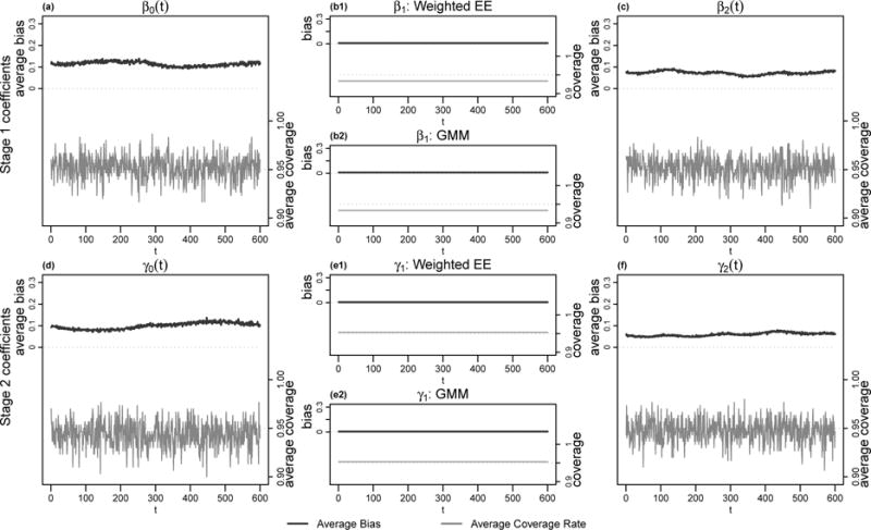
Average bias and average coverage rate for each parameter with N = 600 and T = 600. The black curves depicted the average bias at each t for each parameter, while the corresponding average coverage rates at each t are displayed as light gray vertical bars below. Estimates of the time-invariant parameters using weighted estimation equation and GMM are displayed separately.

Table 1 provides MISE and average coverage rate across t, while using either weighed estimation equation or GMM to estimate the time-invariant parameters. When holding T constant and increasing the sample size N from 300 to 600, MISE drops noticeably (by about a half). When holding N constant and increasing T from 300 to 600, MISE of time-varying coefficients remains about the same but that of time-invariant coefficients decreases substantially. On the other hand, the coverage rate always remains close to 0.95 in all 4 of our scenarios. The weighted estimation equation method exhibited smaller bias but better coverage rate than GMM when estimating β₁ and γ₁.

Table 1.

Mean integrated squared error $\mathit{MISE}=\frac{1}{TR}{\displaystyle {\sum }_{r=1}^R\left[{\displaystyle {\sum }_{t=1}^T{\left\{\eta \left(t\right)-{\widehat{\eta }}_r\left(t\right)\right\}}^2}\right]}$ and average coverage rate across t using weighted estimation equation and GMM method. N = 300 and 600.

			β0(t)	β1	β2(t)	γ0(t)	γ1	γ2(t)
N = 300, T = 300	W/t EE	MISE	3.9 × 10−2	4.6 × 10−4	1.7 × 10−2	1.3 × 10−2	1.6 × 10−4	5.2 × 10−3
		Coverage	95.6%	96.0%	95.5%	94.5%	93.7%	94.7%
	GMM	MISE	3.9 × 10−2	6.5 × 10−4	1.7 × 10−2	1.3 × 10−2	3.2 × 10−4	5.2 × 10−3
		Coverage	95.6%	92.7%	95.5%	94.5%	94.3%	94.7%
			β0(t)	β1	β2(t)	γ0(t)	γ1	γ2(t)
N = 300, T = 600	W/t EE	MISE	4.1 × 10−2	2.5 × 10−4	1.7 × 10−2	1.4 × 10−2	7.7 × 10−5	5.0 × 10−3
		Coverage	95.5%	94.3%	95.5%	94.5%	97.0%	94.6%
	GMM	MISE	4.1 × 10−2	3.9 × 10−4	1.7 × 10−2	1.4 × 10−2	1.5 × 10−4	5.0 × 10−3
		Coverage	95.5%	92.3%	95.5%	94.5%	95.0%	94.6%
			β0(t)	β1	β2(t)	γ0(t)	γ1	γ2(t)
N = 600, T = 300	W/t EE	MISE	2.0 × 10−2	2.0 × 10−4	8.6 × 10−3	7.0 × 10−3	7.6 × 10−5	2.6 × 10−3
		Coverage	95.4%	97.0%	95.1%	94.7%	96.3%	94.7%
	GMM	MISE	2.0 × 10−2	2.5 × 10−4	8.6 × 10−3	7.0 × 10−3	1.4 × 10−4	2.6 × 10−3
		Coverage	95.4%	96.0%	95.1%	94.7%	96.3%	94.7%
			β0(t)	β1	β2(t)	γ0(t)	γ1	γ2(t)
N = 600, T = 600	W/t EE	MISE	2.1 × 10−2	1.4 × 10−4	8.4 × 10−3	7.1 × 10−2	5.3 × 10−5	9.0 × 10−5
		Coverage	95.2%	95.0%	95.2%	94.7%	93.7%	94.7%
	GMM	MISE	2.1 × 10−2	1.8 × 10−4	8.4 × 10−3	7.1 × 10−2	9.0 × 10−5	9.0 × 10−5
		Coverage	95.2%	93.3%	95.2%	94.7%	95.7%	94.7%

5. Application

The Baltimore Longitudinal Study of Aging (BLSA), funded and operated by the National Institute of Aging (NIA), is a study of normative human aging established in 1958 and continuing to this day. Briefly, BLSA continuously enrolls community volunteers as subjects who pass a series of health and functional evaluations. All participants are followed for life and visited every one to four years depending on age. More detailed description of the study could be found in (Ferrucci, 2008). The sample for the current study consists of men and women who underwent a physical examination, health history, and comprehensive energy expenditure testing during their visit between September 2007 and August 2015. The participants were admitted to the Clinical Research Branch unit of the National Institute on Aging for 3 days of testing. Height and weight were assessed in light clothing using a stadiometer and calibrated scale, respectively. Date of birth (age) was derived from a health history interview conducted by trained technicians. On the last day of the visit, participants were asked to wear the Actiheart (CamNtech Ltd, Papworth, UK) device attached on the chest using two standard electrodes. The device collected both heart rate and activity counts in one-minute epochs for the subsequent 7 days in the free-living environment, and was returned to NIA via FedEx.

The data used in this paper were collected from 878 participants who had at least 3 full days of monitoring of their physical activity. More specifically, the data for each subject are minute-by-minute time series of Activity Count (AC). More intense activity tends to correspond to higher AC, at least as measured at the chest level. An AC value of 0 count corresponds to no activity detected. We start by denoting the observed AC of subject i (= 1, 2, …, I) during the t^th minute of day d (= 1, 2, …, D_i) by $Y_{id}^0\left(t\right)$, t = 1, 2, …, 1440. In this data analysis, we only included the most active day (in terms of daily average AC) during each visit for each subject. Specifically, we defined $Y_i\left(t\right)=Y_{id\ast }^0\left(t\right)$ where $d\ast =\underset{d\in \left\{1,2,\dots ,D_i\right\}}{\arg max}[{\displaystyle {\sum }_{t-0}^T{Y}_{id}^0\left(t\right)}]$ for each subject i at time t. To these data we apply the two-stage model described in Section 2 and investigate the association between demographic factors and level of activity in the past one hour and current level of activity at each time of day. The demographic factors in our analysis were time-independent: age (centered at 70), gender (male as 1) and BMI (centered at 27). The minute by minute heart rate H_i(t) (centered at 72) was included as time-dependent covariates. These covariates are basic demographic variables which might only partially account for the population heterogeneity of baseline physical activity. There are many other factors that might affect the baseline physical activity, such as the fitness level, seasonality, geographical location and so on. We only included basic demographics and heart rate to keep this section compact and focus on illustrating application of the two-stage model. We start with modeling all coefficients as time-varying.

Figure 4 presents the estimated coefficients of the two-stage model applied to BLSA. The first two rows of the figure depict the coefficient curves at each time t for the Stage 1 model, while the next two rows display the estimated coefficients for the Stage 2 model. The solid and dotted curves provide LOWESS smoothers for the estimated coefficients. The light gray shades surrounding the estimated coefficients are pointwise bootstrapped 95% confidence bands, which were obtained from LOWESS smoothed coefficients estimated using bootstrapped samples. Figure 4(a) and (f) illustrate the pattern of the intercept for Stage 1 and 2 models, respectively. Figure 4(a) indicates that, on average, a 70-year old woman with a BMI of 27 and heart rate of 72 is less likely to be active during the night (6PM–8AM), but roughly maintains a 60% probability of being active during the daytime from 8AM to 8PM. Figure 4(f) complements Figure 4(a), suggesting that if the same group of women are active during daytime then the intensity of their activity declines, on average, starting from 12PM. Figures 4(b) and 4(g) display the time-varying Stage 1 and Stage 2 coefficients for the minute by minute heart rate. Both coefficients indicate a positive association for the odds of moving and for activity count at every time t. Figure 4(b) indicates that one unit of increased heart rate is associated to greater odds of being active at night and earlier morning compared to day time. However, the Stage 2 coefficient in Figure 4(g) exhibits a more consistent day/night pattern. Figures 4(c) and 4(h) display the effect of age as a function of time during the day for the Stage 1 and Stage 2 models. Together, they indicate that older individuals are more likely to move during the night and early morning periods, though they are less likely to move after 12PM. If they do engage in physical activity then their activity level is, on average, lower in the afternoon and evening (12PM to 22PM). There is also a large increase of the negative effect around 6PM in panel 4(h), which suggests that the largest reduction in activity level for older individuals happens in late afternoon. Results indicate that physical activity interventions may be more effective at increasing overall daily activity if they are targeted towards the second part of the day. Figure 4(d) and (i) illustrate the gender effect. They indicate that the odds of being active is roughly the same for men and women during the day but it is substantially higher for men during the night. In addition, when comparing active men and active women, the level of activity is consistently higher for men throughout day. Because the sex effect seems to depend only on the day or night period, we further considered two time-invariant sex effects, one for day and one for night time. Figure 5 displays the various sex effect estimates. Panel (a) and (d) show the time-varying gender effect as in Figure 4. The weighted estimation equation (panels (b) and (e)) and the GMM method (panels (c) and (f)) both yielded a negative stage 1 effect at night, roughly zero stage 1 effect at daytime and a significant stage 2 effect throughout the day; these results are consistent with our observation from Figure 5(a) and (d). As more information across t was taken into account to estimate the time-invariant sex effect, we chose to leave it in the final model.

Figure 4.

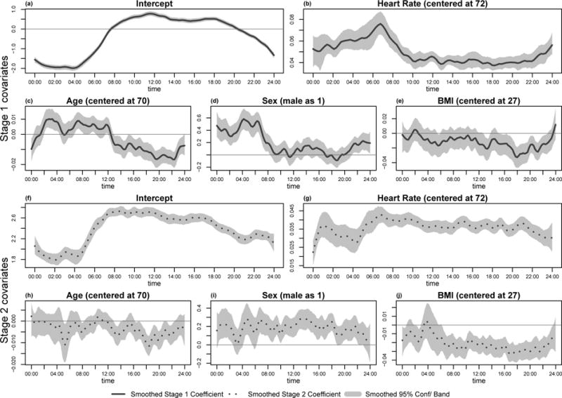
Estimated covariate coefficients of Stage 1 and 2 models. Solid curves depict LOWESS smoothed coefficients of the Stage 1 model, while light gray shadows stand for pointwise bootstrapped 95% confidence interval. Dotted curves and the surrounding light gray shadows follow the same illustration, but for Stage 2 model.

Figure 5.

Comparison of estimated coefficients of gender: as time-varying effect in (a) and (d); as time-invariant coefficient estimated via weighted estimation equation in (b) and (e); as time-invariant coefficient estimated via GMM in (c) and (f). The time-invariant coefficients were fitted separately for the nighttime (0AM–8AM) and daytime (otherwise). Solid and dotted curves depict LOWESS smoothed coefficients of the Stage 1 and Stage 2 model, respectively. The light gray shadows surrounding the estimated coefficients stand for pointwise bootstrapped 95% confidence bands.

6. Discussion

We introduced a two-stage model for a general type subject-specific, dense time series data with excess zeros. Such data are typical in studies using wearable devices. The model describes the effect of covariates on the occurrence of events and, conditional on the fact that the event occurred, it describes the effect of covariates on the magnitude of response. A logistic regression model was introduced to account for the first stage of the model, and a log-linear model was used for the second stage of the model. While both models are relatively well known, the novel combination, the application to high density wearable computing data, and the extension of zero-inflated models to time series make our approach novel. Most importantly, such approaches are absolutely crucial to uncover the type of findings we have shown in Section 5, for generating hypothesis, and for suggesting simpler, easier to understand models.

Our scientific findings are both striking and reasonable. To our knowledge, this is the first time when the effect of covariates’ is separated according to probability of being active and the level of activity. Moreover, going from qualitative statements about possible associations that seem reasonable to a reader to quantifying these associations is often the difference between research and hearsay. We have shown that some covariates affect the odds of being active while others only affect the level of activity. Such separation of the covariate effect is important, as researchers may start to disentangle the “will” and “ability” of being active. Note, for example, that in-lab experiments often have a very difficult time distinguishing between two equally able individuals who have a very different levels of motivation to be active. In the lab both would perform equally well. In the natural living environment things can be completely different. Ultimately, this could provide valuable information in terms of targeting interventions and understanding the complex nature of interactions between physiological and psychological determinants of activity and health. Our work has laid a foundation for more systematic ways of analyzing wearable computing data in the future.

Our method has several limitations that could be further addressed in future studies. First, we did not assume independence across t because the two-stage model is a marginal model which treats correlations across t as nuisance parameters. In the future, it would be of great interest to develop statistical techniques that could take advantage of, for example, local correlations from repeated measurements (across t) to improve estimation efficiency. Second, we only used one day of accelerometry data within each multiple-day visit. An important extension would be to develop methods that take into account the correlation structure of physical activity profiles across several days within each visit. Third, we estimated each time-varying coefficient at every t and smoothed them afterwards. An alternative way could be to introduce smoothing directly during the estimation. For example, a set of q-dimensional B-spline basis functions might be used to effectively reduce the number of parameters for one covariate from T to q, where q ≪ T is the number of parameters of the spline. Moreover, one could use periodic splines to better capture the periodic behavior of coefficients and ensure that the same value is estimated at the start (0AM) and end (24PM) of the day. This may further reduce the standard error of time-varying coefficients close to the middle of the night.

References

- Bai J, Di C, Xiao L, Evenson KR, LaCroix AZ, Crainiceanu CM, Buchner DM. An Activity Index for raw accelerometry data and its comparison with other activity metrics. PLoS ONE. 2016;11:e0160644. doi: 10.1371/journal.pone.0160644. [DOI] [PMC free article] [PubMed] [Google Scholar]
- Bai Y, Welk GJ, Nam YH, Lee JA, Lee JM, Kim Y, Meier NF, Dixon PM. Comparison of consumer and research monitors under semistructured settings. Medicine and Science in Sports and Exercise. 2016;48:151–158. doi: 10.1249/MSS.0000000000000727. [DOI] [PubMed] [Google Scholar]
- Brage S, Brage N, Franks PW, Ekelund U, Wareham NJ. Reliability and validity of the combined heart rate and movement sensor Actiheart. European Journal of Clinical Nutrition. 2005;59:561–570. doi: 10.1038/sj.ejcn.1602118. [DOI] [PubMed] [Google Scholar]
- Ferrucci L. The Baltimore Longitudinal Study of Aging (BLSA): a 50-year-long journey and plans for the future. The journals of gerontology. Series A, Biological sciences and medical sciences. 2008;63:1416–9. doi: 10.1093/gerona/63.12.1416. [DOI] [PMC free article] [PubMed] [Google Scholar]
- Goldsmith J, Zipunnikov V, Schrack J. Generalized Multilevel Functional-on-Scalar Regression and Principal Component Analysis. Biometrics. 2015;71:344–353. doi: 10.1111/biom.12278. [DOI] [PMC free article] [PubMed] [Google Scholar]
- Hansen LP. Large Sample Properties of Generalized Method of Moments Estimators. Econometrica. 1982;50:1029. [Google Scholar]
- John D, Freedson P. ActiGraph and actical physical activity monitors: A peek under the hood. Medicine & Science in Sports & Exercise. 2012;44:S86–S89. doi: 10.1249/MSS.0b013e3182399f5e. [DOI] [PMC free article] [PubMed] [Google Scholar]
- Li H, Kozey Keadle S, Staudenmayer J, Assaad H, Huang JZ, Carroll RJ. Methods to assess an exercise intervention trial based on 3-level functional data. Biostatistics. 2015;16:754–771. doi: 10.1093/biostatistics/kxv015. [DOI] [PMC free article] [PubMed] [Google Scholar]
- Li H, Staudenmayer J, Carroll RJ. Hierarchical functional data with mixed continuous and binary measurements. Biometrics. 2014;70:802–811. doi: 10.1111/biom.12211. [DOI] [PubMed] [Google Scholar]
- Neilson HK, Robson PJ, Friedenreich CM, Csizmadi I. Estimating activity energy expenditure: How valid are physical activity questionnaires? American Journal of Clinical Nutrition. 2008;87:279–291. doi: 10.1093/ajcn/87.2.279. [DOI] [PubMed] [Google Scholar]
- Pinsky M, Karlin S. An Introduction to Stochastic Modeling. 4th Academic Press; 2010. [Google Scholar]
- Schrack JA, Zipunnikov V, Goldsmith J, Bai J, Simonsick EM, Crainiceanu C, Ferrucci L. Assessing the “Physical Cliff”: Detailed quantification of age-related differences in daily patterns of physical activity. The Journals of Gerontology Series A: Biological Sciences and Medical Sciences. 2014;69:973–979. doi: 10.1093/gerona/glt199. [DOI] [PMC free article] [PubMed] [Google Scholar]
- Shou H, Zipunnikov V, Crainiceanu CM, Greven S. Structured functional principal component analysis. Biometrics. 2015;71:247–257. doi: 10.1111/biom.12236. [DOI] [PMC free article] [PubMed] [Google Scholar]
- Terbizan DJ, Dolezal Ba, Albano C. Validity of seven commercially available heart rate monitors. Measurement in Physical Education and Exercise Science. 2002;6:243–247. [Google Scholar]
- Vähä-Ypyä H, Vasankari T, Husu P, Mänttäri A, Vuorimaa T, Suni J, Sievänen H. Validation of cut-points for evaluating the intensity of physical activity with accelerometry-based Mean Amplitude Deviation (MAD) PLOS ONE. 2015;10:e0134813. doi: 10.1371/journal.pone.0134813. [DOI] [PMC free article] [PubMed] [Google Scholar]
- Xiao L, Huang L, Schrack JA, Ferrucci L, Zipunnikov V, Crainiceanu CM. Quantifying the lifetime circadian rhythm of physical activity: a covariate-dependent functional approach. Biostatistics. 2015;16:352–367. doi: 10.1093/biostatistics/kxu045. [DOI] [PMC free article] [PubMed] [Google Scholar]
- Yang CC, Hsu YL. A review of accelerometry-based wearable motion detectors for physical activity monitoring. Sensors. 2010;10:7772–7788. doi: 10.3390/s100807772. [DOI] [PMC free article] [PubMed] [Google Scholar]
Associated Data
This section collects any data citations, data availability statements, or supplementary materials included in this article.