Coordinating AgMIP data and models across global and regional scales for 1.5°C and 2.0°C assessments

Abstract

The Agricultural Model Intercomparison and Improvement Project (AgMIP) has developed novel methods for Coordinated Global and Regional Assessments (CGRA) of agriculture and food security in a changing world. The present study aims to perform a proof of concept of the CGRA to demonstrate advantages and challenges of the proposed framework. This effort responds to the request by the UN Framework Convention on Climate Change (UNFCCC) for the implications of limiting global temperature increases to 1.5°C and 2.0°C above pre-industrial conditions. The protocols for the 1.5°C/2.0°C assessment establish explicit and testable linkages across disciplines and scales, connecting outputs and inputs from the Shared Socio-economic Pathways (SSPs), Representative Agricultural Pathways (RAPs), Half a degree Additional warming, Prognosis and Projected Impacts (HAPPI) and Coupled Model Intercomparison Project Phase 5 (CMIP5) ensemble scenarios, global gridded crop models, global agricultural economics models, site-based crop models and within-country regional economics models. The CGRA consistently links disciplines, models and scales in order to track the complex chain of climate impacts and identify key vulnerabilities, feedbacks and uncertainties in managing future risk. CGRA proof-of-concept results show that, at the global scale, there are mixed areas of positive and negative simulated wheat and maize yield changes, with declines in some breadbasket regions, at both 1.5°C and 2.0°C. Declines are especially evident in simulations that do not take into account direct CO₂ effects on crops. These projected global yield changes mostly resulted in increases in prices and areas of wheat and maize in two global economics models. Regional simulations for 1.5°C and 2.0°C using site-based crop models had mixed results depending on the region and the crop. In conjunction with price changes from the global economics models, productivity declines in the Punjab, Pakistan, resulted in an increase in vulnerable households and the poverty rate.

This article is part of the theme issue ‘The Paris Agreement: understanding the physical and social challenges for a warming world of 1.5°C above pre-industrial levels'.

1. Introduction

Agricultural practices influence global climate change through emissions of greenhouse gases by land clearing, land-use change, animal husbandry, fertilizer application, tillage practices, fuel use and rice cultivation. At the same time, agriculture is affected by climate change at the within-country local-to-regional scale through effects of heatwaves, droughts and floods. Reduction of greenhouse gases through the agricultural sector is included in the Nationally Determined Contributions (NDCs) of many countries, and agricultural impacts are a major source of vulnerability and also a prime focus of many National Adaptation Plans (NAPs). How will global climate change processes and policies affect regional agriculture, and how does regional agriculture in turn affect the global scale? In this paper, we describe the goals, methodology and status of the Agricultural Model Intercomparison and Improvement Project (AgMIP) [1] Coordinated Global and Regional Assessments (CGRA) [2,3] proof of concept and its initial methodology using Half a degree Additional warming, Prognosis and Projected Impacts (HAPPI) [4] climate scenarios and the Coupled Model Intercomparison Project Phase 5 (CMIP5) [5] transient simulations to respond to the request by the UN Framework Convention on Climate Change (UNFCCC) for information about the implications of limiting global temperature increases to 1.5°C and 2.0°C [6].

AgMIP began in 2010 and involves approximately 1000 climate scientists, crop and livestock experts, economists and information technology specialists who conduct protocol-based activities to significantly improve projections of agricultural responses to major stresses [1]. The motivation for the CGRA comes from the multi-model ensembles of biophysical and socio-economic simulations done by AgMIP scientists, which have enabled extensive model intercomparison at, but generally not across, a range of scales based on farm-site networks and global grids (see also [7]). AgMIP continues to focus on model improvements through protocol-based research on agricultural system components, including individual crops (e.g. wheat, maize, rice, sugarcane, canola and potatoes), soils, and pests and diseases. The complementary goal is to advance learning on the interactions of agricultural mitigation and adaptation by focusing on explicit and testable linkages across disciplines and scales. This is in contrast to the embedding of reduced forms of these linkages in integrated assessment models (IAMs) [8,9]. To date, most agricultural modelling has addressed research questions within particular disciplines and scales (for exceptions related to policy assessment, see [10–12]).

At the large scale, the AgMIP Gridded (AgGrid) crop modelling initiative, largely through its flagship Global Gridded Crop Model Intercomparison (GGCMI) project, has evaluated more than a dozen global crop models in historical validation tests, coordinated climate impact assessments, and conducted sensitivity and uncertainty studies [13–15]. Individual crop intercomparisons (e.g. wheat, maize, rice, sugarcane, canola and potatoes) have tested many models, with projects sometimes attracting as many as 30–40 different researchers, at multiple sites around the world [16–19]. In close collaboration with the climate and crop-growth modellers, the AgMIP Global Economics Team has analysed and compared the economic consequences of different climate change impact and mitigation scenarios by means of more than 10 global economics models [20–22]. Interdisciplinary agricultural research at the global scale has been mainly constrained to the monodirectional information flow from biophysical crop modelling to economic modelling [20,23]. This approach has enabled changes in crop yields at the global scale to be evaluated in terms of price and welfare effects. Coupled exploration for IAMs has been proposed using simplified climate and crop emulators informed by AgMIP results [7].

At the regional scale (defined as within-country agricultural areas), the AgMIP Regional Integrated Assessment (RIA) project in sub-Saharan Africa and South Asia has developed new methods to conduct stakeholder-driven research linking climate, crop, livestock and economics models on impacts and adaptation in current and future climates [24–27]. In this approach, multiple site-based crop models simulate the impacts of representative future climate scenarios, and regional economics models are employed to test farmer responses to climate-driven crop yield changes and to assess vulnerabilities of farm households.

In AgMIP CGRA, we build on this body of work by coordinating major modelling initiatives across disciplines and scales through the use of unified climate, socio-economic and agronomic assumptions [28–30]. Such explicit disciplinary and scale interactions enable improvements in simulated processes, such as improved crop yield projections for embedding in economics models, and validation for results from aggregated global models that may be interpreted meaningfully for the regions where agriculture represents a significant share of the economy. A multi-year process has created a conceptual framework for assessing global- and regional-scale modelling of crops, livestock and economics across major agricultural regions worldwide (figure 1) [2,3]. This CGRA framework is designed to facilitate the production of consistent multi-model, multidiscipline and multiscale assessments of agricultural and food security impacts, including robust characterizations of uncertainty and risk.

Figure 1.

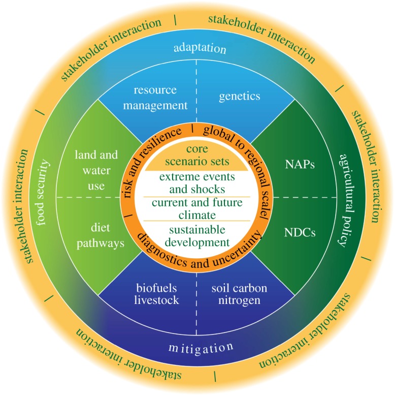
CGRA climate and food research framework to provide guidance for agricultural adaptation, mitigation, food security and agricultural policy. (Online version in colour.)

In the CGRA framework, there are four dimensions: adaptation, mitigation, food security and agricultural policy. The context for these dimensions involves extreme events and shocks, current and future climate, and sustainable development. The overall research question is: How can the world's food system respond to climate change, as well as other shocks, such as economic crises and conflicts, in the context of sustainable development? Different initiatives within AgMIP address this and related questions by leveraging data and models to forecast regional and global food systems across time scales ranging from in-season monitoring to multi-decadal impacts [13,16,24]. The AgMIP consortium is also working with nutrition scientists to incorporate metrics into assessments that go well beyond just calories, including dietary intake and nutrients [3]. Potential topics for CGRA assessments are: evaluations of adaptations such as genetics and resource management [31]; mitigation options including biofuels, soil carbon, nitrogen management and livestock system transitions [32]; food security issues such as diet standards and land use [33]; and agricultural policy questions related to NDCs and NAPs as well as import/export controls and public subsidies [34].

Different degrees of coordination can be identified across the CGRA assessment activities (see the first table in appendix A) from loosely coordinated to directly linked. ‘Loosely coordinated’ studies share a common set of climate, socio-economic and agronomic scenarios and assumptions. This enables comparative analysis of results across a wide range of studies. ‘Directly linked’ studies explicitly provide model outputs from one discipline and/or scale to be applied as inputs to other models from another discipline and/or scale.

The present study aims to perform a proof of concept of the CGRA for 1.5°C and 2.0°C of global warming above pre-industrial conditions, demonstrating advantages and challenges of the proposed framework. Here, we describe the key scenario assumptions, model components and major uncertainties in the CGRA framework prototype application. Ruane et al. (see row A in the first table in appendix A, and ref. [2]) provide details of the full AgMIP CGRA for 1.5°C and 2.0°C warming.

2. Scenarios and models

(a). Climate scenarios

AgMIP CGRA research is being conducted using a wide range of climate and socio-economic scenario approaches [2]. One scenario approach embedded in AgMIP CGRA 1.5°C/2.0°C research is based on CMIP5 transient simulations of twenty-first century climate changes for Representative Concentration Pathway RCP4.5 [5]. This RCP4.5 transient approach allows a more explicit coupling of time frame and climate projections in the CGRA analyses. Another approach is the use of bias-corrected climate scenarios from 20-member ensembles of three HAPPI global climate models (GCMs), which enables an extensive assessment of impacts of extreme weather events in the agricultural sector at 1.5°C and 2.0°C [4,35].

The HAPPI simulations aim to reproduce the stabilized climate at 1.5°C or 2.0°C above pre-industrial conditions, which stands in contrast to the RCP4.5 transient simulations that represent an emissions pathway developed for CMIP5. RCP4.5 was not designed to reach a specific climate stabilization and, therefore, application requires the identification of time periods within each GCM where global temperature is approximately 1.5°C or 2.0°C above pre-industrial conditions. Not all such GCM simulations achieve 2.0°C global warming, and those that do reveal an evolving climate trajectory in which a steady climatology is hard to characterize.

RCP2.6 transient runs help to explore one potential pathway for mitigation, underscoring the likelihood of a peak and decline in global temperatures for high-mitigation futures. The AgMIP Climate Team is comparing RCP2.6 and HAPPI [2], and some related CGRA projects are using RCP2.6 (see row B in the first table in appendix A). AGCLIM50 Phase 2 is employing RCP1.9 for the 1.5°C climate realization and RCP2.6 for the 2.0°C climate realization [22].

(b). Socio-economic scenarios: Shared Socio-economic Pathways and Representative Agricultural Pathways

Shared Socio-economic Pathways (SSPs) and Representative Agricultural Pathways (RAPs) provide global and regional trajectories of non-climate factors for the analyses (see the second table in appendix A). The SSPs set the macro- and socio-economic global context with some agricultural information, but agricultural trends differ in the different realizations of the marker scenarios [29,36]. RAPs are agriculture-specific extensions of the SSPs envisaging future agricultural policy and development for global and regional analyses [30]. At the regional level, the development of RAPs enables direct linkages to stakeholders, representation of different farming systems, and inclusion of analysis of many more variables, such as vulnerable farm households, livelihoods and poverty [30,37].

(c). Global and regional crop models

Global-scale evaluation of crop productivity is a major challenge for climate impact and adaptation assessment. Rigorous global assessments that are able to inform planning and policy-making benefit from consistent input data and assumptions across regions and time that use mutually agreed protocols designed by the modelling community [38]. The AgMIP GGCMI has built a community of researchers that collaborate to perform coordinated global and regional high-resolution impact assessments and model intercomparison studies. In turn, these improve GGCMI applications and understanding of climate impacts on global food production, as well as regional and temporal variations in these responses. For a list of global crop modelling being done for the CGRA study, see the first table in appendix A.

For crops at the regional scale in CGRA, AgMIP works with the Decision Support System for Agrotechnology Transfer (DSSAT) and the Scientific Impact assessment and Modelling Platform for Advanced Crop and Ecosystem management (SIMPLACE). DSSAT, which comprises crop simulation models for over 42 crops (as of v.4.6), is supported by database management programs for soil, weather, and crop management and experimental data, and by utilities and application programs [39,40]. The crop models in DSSAT simulate growth, development and yield as a function of soil–plant–atmosphere dynamics, and they have been adopted for many applications ranging from on-farm management to regional assessments of the impacts of climate variability and climate change. DSSAT has been in operation for more than 20 years by researchers, educators, consultants, extension agents, growers, and policy- and decision-makers in over 100 countries worldwide. SIMPLACE uses modular software architecture within standard technologies, which reduces the effort in model development and customization. The multithreaded high-performance architecture enables calibration and simulations at different spatial scales [41].

GGCMI simulations were conducted using stabilization scenarios with bias-corrected daily input of HAPPI GCMs [4]. The trend-preserving bias-correction method [42] applied is adopted from the Inter-Sectoral Impact Model Intercomparison Project (ISIMIP2b) protocol [43]. These simulations calculated crop productivity for 600 years (3 GCMs × 20 ensemble members × 10 years each) for the present and future (1.5°C and 2.0°C) with GGCMI models and protocols. The large sample of simulation years allows for analysis of extreme yield losses and changes in the distribution of crop productivity in the baseline and the 1.5°C and 2.0°C scenarios (see row I in the first table in appendix A).

(d). Global and regional economics models

The role of global economics models in this study is to anticipate economic responses to changes in crop productivity, including changes in cropland area, crop mix, imports, exports, production, consumption and prices [20]. The current global system generally shows little flexibility in total crop consumption patterns compared with a future world without climate changes, adjusting all other economic variables to motivate production that satisfies demand and substituting abundant crops where similar crops had lower production totals. Changes in economic variables, specifically world prices of crops, are made available to the regional economics models. The CGRA proof-of-concept study utilizes the International Model for Policy Analysis of Agricultural Commodities and Trade (IMPACT) partial equilibrium model [44] and the Future Agricultural Resources Model (FARM) computable general equilibrium model [45].

AgMIP applies the Trade-Off Analysis model for Multi-Dimensional impact assessment (TOA-MD) [46,47] to implement the regional economic analysis for CGRA. The TOA-MD model is a parsimonious, generic model for analysis of technology adoption and impact assessment, and ecosystem services analysis. The TOA-MD model was designed to simulate technology adoption and impact in a population of heterogeneous farms. In the TOA-MD model, farmers are presented with a binary choice: they can operate with a current or base production system 1, or they can switch to an alternative system 2.

In a technology adoption and impact analysis, the model simulates the proportion of farms that would adopt the new or alternative system, as well as the impacts of the new system by simulating impact indicators defined by the user. The choice of system is based on the distribution of expected economic returns in the farm household population, so the predicted adoption rate can be interpreted as the rate that is economically feasible. The model can simulate the full range of adoption rates from zero to 100%, and thus can be helpful in studying impacts if other factors (e.g. financial or behavioural) constrain adoption. Impacts are estimated based on the statistical relationship between expected returns to the alternative system and outcome variables (e.g. economic, environmental or social outcomes). Regional prices are taken from the AgMIP global economics models for the different SSPs and/or mitigation scenarios.

The TOA-MD model assesses climate impacts by using an analogy to technology adoption. Farms cannot choose whether to have climate change or not, but if farms had such a choice, those that would choose to ‘adopt’ climate change are those who would gain from it; farms that would prefer not to ‘adopt’ climate change are those who would lose from it. An important implication of this model, when predicting a technology adoption rate, is that the rate is typically above zero and below 100%—it is rare for all farms to adopt a technology because in a heterogeneous population not all farms perceive it to be beneficial. The analogy to climate impact assessment is that there are typically both losers and gainers from climate change. The phenomenon of losers and gainers from climate change can be explained (at least in part) by the heterogeneity in the conditions in which the farms operate, such as soils, water resources, topography, climate, the farm household's socio-economic characteristics, and the broader economic, institutional and policy setting [48].

3. Proof-of-concept assessment

Figure 2 and table 1 show the explicit linkages for the elements of the CGRA 1.5°C and 2.0°C HAPPI proof-of-concept assessment.

Figure 2.

CGRA framework for HAPPI 1.5°C and 2.0°C proof-of-concept assessment (Δ = change). (Online version in colour.)

Table 1.

Regions analysed for each discipline in the CGRA proof-of-concept study (see the first table in appendix A for further analyses).

	Punjab, Pakistan	Nioro, Senegal	US Pacific Northwest	Global
climate	✓	✓		✓
crops	✓	✓		✓
economics	✓		✓	✓

(a). Global scale

The global-scale simulations tested future 1.5°C and 2.0°C climate scenarios with and without mitigation policies (i.e. a carbon tax).

(i). Global climate scenarios

HAPPI climate simulations are the anchor of the proof-of-concept assessment, with results compiled from large (83–500 members) ensembles from five global climate modelling groups (see row B in the first table in appendix A, and refs [2] and [4]). HAPPI provides a framework for the generation of climate data describing how the climate, and in particular extreme weather, might differ from the present day in worlds that are 1.5°C and 2.0°C warmer than pre-industrial conditions [4]. AgMIP CGRA has selected 2050 as the timing to be associated with the HAPPI climate projections [2], in order to enable associated economic model simulations. This falls among the more rapid stabilization curves projected to achieve 1.5°C or 2.0°C climate realizations [49].

The HAPPI results were processed to provide ensemble mean monthly change patterns for 1.5°C and 2.0°C for maximum and minimum temperature (and their standard deviations), precipitation and number of rainy days. HAPPI climate projections provide the basis for regional climate scenarios generated in combination with local observations following the AgMIP Climate Scenario Protocols [25], as well as global scenarios for growing-season average temperature and precipitation changes for each of the four major crops (wheat, maize, rice and soya bean) for global crop model sensitivity analyses [2]. Figure 3 presents climate scenarios for wheat under 2.0°C across the ensemble median for all five HAPPI GCMs, revealing substantial regional differences (particularly for precipitation change projections) (see electronic supplementary material, figure S1 for climate scenarios for 2.0°C rainfed maize). Comparisons between HAPPI and transient simulations from CMIP5 [5] show that overall projections are consistent with a subset of the larger CMIP5 model ensemble [2].

Figure 3.

Climate scenarios for rainfed wheat growing season under the 2.0°C climate realizations across five HAPPI GCMs. (a–e) Changes in temperature and (f–j) changes in precipitation. Grid cells with less than 10 ha of wheat not shown.

Climate scenarios and assumptions within this CGRA proof-of-concept study are consistent with the HAPPI guidelines to the extent possible (table 2). Bias-corrected HAPPI climate scenarios provide additional realism due to substantial differences in extreme events between the 1.5°C and 2.0°C climate realizations [4,35]. Climate scenarios in the proof-of-concept CGRA global crop simulations do not include explicit changes in extreme events, and therefore the effects of changes in extremes are not reflected in the economics model results.

Table 2.

Climate scenarios and assumptions of the AgMIP HAPPI proof-of-concept study.

HAPPI pre-industrial period	1861–1880
Baseline observed climate
GGCMI current period	1980–2009
HAPPI current period	2006–2015
CO2 concentration levels
HAPPI current period	390 ppm
HAPPI 1.5°C	423 ppm
HAPPI 2.0°C	487 ppm
HAPPI future time frame	2106–2115
AgMIP CGRA current time frame	2010
AgMIP CGRA future time frame	2050
GCMs	CAM4-2°, CanAM4, HadAM3P, MIROC5, NorESM1
	83–500 ensemble members, each running 10 years for each period

(ii). Global crops

To project changes in crop yields at the global scale, multi-model ensembles were developed from HAPPI climate realizations and AgMIP GGCMI results. The HAPPI mean growing-season temperature and precipitation changes were located on yield response surfaces developed from AgMIP GGCMI sensitivity tests conducted under combinations of changes to CO₂, temperature, water and nitrogen [2,7,13]. Results for the four major crops were projected for five GCMs under rainfed and irrigated growing conditions for 1.5°C and 2.0°C climate realizations, holding nitrogen levels at present conditions. Figure 4 shows rainfed wheat changes for the 2.0°C HAPPI scenario (see electronic supplementary material, figure S2 for the same results for rainfed maize). Regional differences are evident across the GCMs, but large-scale patterns are strongly influenced by the global gridded crop model (GGCM). In general, in the 2.0°C climate realization with CO₂ effects, wheat increases in the Pacific Northwest, southern Europe and northern China, while reductions are seen in the North American interior, northern Eurasia, South Asia and most Southern Hemisphere production regions. The Lund–Potsdam–Jena managed Land (LPJmL) model is optimistic given its beneficial representation of CO₂ processes.

Figure 4.

Projected rainfed wheat yield change (compared with HAPPI 2006–2015 current period). Columns show different global gridded crop models ((a–e) parallel Decision Support System for Agrotechnology Transfer, pDSSAT; (f–j) Geographic Information System-based Environmental Policy Integrated Climate, GEPIC; and (k–o) Lund–Potsdam–Jena managed Land, LPJmL), and rows show five HAPPI GCMs that provided driving climate projections. Grid cells with less than 10 ha of wheat not shown.

Figure 5 compares differences between the 1.5°C and 2.0°C climate realizations and the three GGCM projections (for the CanAM4 climate scenario) for rainfed wheat with and without direct effects of CO₂ (see electronic supplementary material, figure S3 for results for rainfed maize). When direct effects of CO₂ are taken into account, yield is higher in 2.0°C compared to 1.5°C in many locations due to the effect of higher CO₂ concentrations. In simulations without CO₂ effects, crop yields associated with 2.0°C are lower in many regions of the world than with 1.5°C. The range between these projections represents the limits of uncertain CO₂ effects across different crop species and farming systems, which is a persistent challenge for crop models given that experimental results are limited to a relatively small set of regions and conditions [50–53].

Figure 5.

Difference between 2.0°C and 1.5°C rainfed wheat yield with (a–c) and without (d–f) CO₂ effects for three global gridded crop models (pDSSAT, GEPIC and LPJmL) and the CanAM4 HAPPI scenario.

(iii). Global economics

The GGCMI crop yield changes derived from the AgMIP HAPPI 1.5°C and 2.0°C climate scenarios were applied as inputs to the IMPACT and FARM models under future scenarios with and without mitigation policies (the latter imposed through a carbon tax). Figure 6 is an example of these results, showing global price and area changes for maize and wheat under 2.0°C. Results show uncertainty in world commodity price changes without a carbon tax simulated by the two global economics models associated with the exogenous climate shocks produced by the five HAPPI GCMs, each simulated by three GGCMs (GEPIC [54], LPJmL [55] and pDSSAT [56]). Maize prices increase in all three GGCMs in IMPACT, while in the FARM economics model for pDSSAT and GEPIC prices increase and decrease slightly for LPJmL. Wheat prices increase for the pDSSAT and GEPIC simulations, while simulations driven by LPJmL have higher CO₂ effects leading to higher production and a reduction in prices. Maize area increases across all GGCMs and both global economic models. The FARM model has lower wheat price changes than IMPACT, but differs in the associated pressure on land use (small changes except for reduction in wheat area for LPJmL). Results in the FARM model with mitigation show much greater increases in prices (+20% for maize and wheat) and large decreases in crop areas (−16% for maize and −14% for wheat).

Figure 6.

Global economic impacts of 2.0°C climate realization on maize and wheat (a) price and (b) area under an SSP2 2050 scenario with no mitigation, compared with an equivalent scenario without climate impacts. Results presented for IMPACT and FARM global economics models driven by agricultural production changes from three global gridded crop models and five HAPPI GCMs. For comparison, price and area changes are presented from a FARM simulation with no direct climate impacts on agriculture but with a carbon tax implemented to create a 2.0°C pathway.

(b). Regional scale

The motivation for the coordinated simulations at the regional scale are to explore the effects of global mitigation policies (e.g. carbon tax) and local ones (e.g. introduction of biofuel crops and adoption of no-till cultivation), and the impacts of climate change on regional farming systems and farmer livelihoods. Regional approaches also incorporate more detailed information about local climate, cultivars, management and household economics [57].

(i). Regional climate scenarios

HAPPI seasonal changes were imposed on historical observations to create statistically downscaled local climate scenarios for crop model simulations at regional scales utilizing the AgMIP mean-and-variability approach developed for the RIAs in sub-Saharan Africa and South Asia [25]. Historical observations, from either local weather stations or AgMERRA (the Agricultural applications version of the Modern-Era Retrospective analysis for Research and Applications) [58], were adjusted to match the new temperature distributions; the method maintains the shape of the precipitation distribution, while changing the number of rainy days. The result is a 31-year weather series for each GCM scenario (see figure 7 for mean monthly temperature (°C) and mean monthly precipitation (mm) for observed and projected 1.5°C and 2.0°C assessments for Bahawalnagar, Punjab, Pakistan and Nioro, Senegal).

Figure 7.

Local climate projections for Bahawalnagar, Punjab, Pakistan (a,b) and Nioro, Senegal (c,d) from five HAPPI GCMs representing 1.5°C and 2.0°C climate realizations. (Note differences in scales.)

(ii). Regional crops

The AgMIP HAPPI 1.5°C and 2.0°C downscaled climate scenarios were employed in DSSAT simulations for the agricultural regions of the Punjab, Pakistan at five sites (Bahawalnagar, Bahawalpur, Lodhran, Multan and Rahim Yar Khan) and Nioro, Senegal. (The SIMPLACE model was also operated for Senegal.) An additional analysis of farming systems in the US Pacific Northwest used the DeNitrification DeComposition (DNDC) model [59]. Methods (inputs, calibration and validation) for the regional crop and economics model simulations in Pakistan, Senegal and the US Pacific Northwest are described in Ahmad et al. [60], Adiku et al. [61] and Antle et al. [62], respectively.

The CGRA framework allows exploration of uncertainty in projections of the biophysical impacts of HAPPI climate scenarios as simulated by a locally calibrated crop model (DSSAT) and global gridded crop models from GGCMI. Figure 8 compares results from the five GCMs for Punjab wheat and Nioro maize. The global gridded version of DSSAT (pDSSAT) agrees most strongly with the local projections for both regional crops. GEPIC and LPJmL projections are much less pessimistic about maize production, while LPJmL is optimistic about wheat.

Figure 8.

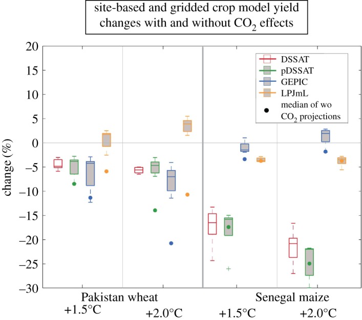
Regional and global yield projections for wheat in Pakistan (mean of five sites) and maize in Senegal. Results presented with CO₂ effects for locally configured DSSAT simulations and corresponding grid cells from global gridded crop models (pDSSAT, GEPIC and LPJmL). Box-and-whiskers represent five HAPPI GCMs and dots represent the median of corresponding simulations without (wo) CO₂ effects.

(iii). Regional economics

The TOA-MD tested the following hypotheses:

• H1: Global mitigation efforts to achieve 1.5°C will have quantifiable impacts on farm households in low- and high-income countries and on achieving sustainable development goals, through effects of mitigation policies and prices (MPP), cost of production, land use and trade (H1 was tested in Punjab, Pakistan).

• H2: In countries with mitigation policies, farm households will benefit from participation in mitigation activities and will contribute to net greenhouse gas mitigation and other sustainable development goals (H2 was tested in the US Pacific Northwest).

The AgMIP RIA approach [27] quantified the impacts of 1.5°C and 2.0°C global warming and global mitigation policies and associated price changes on regional farming systems by answering the following RIA questions:

• Question 1: What are the impacts of global warming (of 1.5°C and 2.0°C) and global mitigation policies and prices on production systems in the near term (i.e. 2030)?

• Question 2: What are the impacts of global warming (of 1.5°C and 2.0°C) and global mitigation policies and prices on future (i.e. 2050) production systems?

Different assumptions in the global economic modelling implemented in IMPACT were used to design a set of scenarios as a sensitivity test for different global price changes on key crops of the farming system. IMPACT results included price and productivity projections to 2030 and 2050 under five GCMs and three global gridded crop models (pDSSAT, GEPIC and LPJmL). The core questions and scenarios design for Punjab, Pakistan are described in table 3.

Table 3.

Scenario design for the 1.5°C and 2.0°C assessments for Punjab, Pakistan implemented with TOA-MD.

	Question 1: 2030a/Question 2: 2050b
scenario	system 1	system 2
scenario 1	no climate change, no major agricultural global mitigation policies	climate change, no major agricultural global mitigation policies
scenario 2	no climate change, no major agricultural global mitigation policies	climate change, agricultural global mitigation policies based on SSP1
scenario 3	no climate change, agricultural global mitigation policies based on SSP1	climate change, agricultural global mitigation policies based on SSP1

^aAssuming no significant change in crop yields due to climate change. Trends to 2030 based on a sustainable development RAP.

^bRegional crop modelling estimated impacts of climate change on crop yields. Trends to 2050 based on a sustainable development RAP.

TOA-MD estimates the changes in key economic indicators such as the average impact on farm income, vulnerability of farm income to loss (e.g. the percentage of the population expected to lose farm income and the magnitude of the losses) and changes in poverty indicators (e.g. headcount poverty rate and poverty gap). Other environmental and social indicators can be included given available data, including changes in food security indicators (e.g. proportion of the population consuming a nutritionally adequate diet) and greenhouse gas emissions.

Punjab, Pakistan. In the Punjab region of Pakistan, output data from a global economics model (i.e. IMPACT) represented the likely impacts of global mitigation policies on wheat and cotton prices under 1.5°C and 2.0°C scenarios by 2030 and 2050 (table 4). The analysis shows that, in the near term, the overall impact of changes in crop yields, prices and costs of production on farm income is small with the 2.0°C, resulting in a slightly negative change in net farm income (between −1% and −3% on average across the different districts in the Punjab region). The longer-term analysis shows a more negative picture for the Punjab region in Pakistan. Between 63 and 73% of households are vulnerable to losses; net farm income might be reduced between 10 and 21%, with net economic losses up to 41% of farm income. These conditions can increase poverty rates by 12–38%, demonstrating that the severity of impacts differs across the five districts tested in the Punjab region. The impacts in the near term (2030) are much smaller than the longer term (2050) when the impacts of climate change on crop yields are larger; price increases also tend to be larger but may not offset yield losses. See figure 8 for regional crop results for Punjab, Pakistan.

Table 4.

Impacts of 1.5°C and 2.0°C global carbon tax on five villages in the Punjab cotton–wheat system in Pakistan simulated by the TOA-MD model. Global economic output data included five GCMs and three global gridded crop models. Results shown are the average across GCMs, crop models and scenarios. Aggregated results for the Punjab region are weighted averages based on the area of each district. Hhs, households.

		near term (2030)				longer term (2050)
climate	region	extent of vulnerability (% vulnerable hhs)	average % change in farm net returns	average economic losses (% of farm net returns)	change in poverty rate (%)	extent of vulnerability (% vulnerable hhs)	average % change in farm net returns	average economic losses (% of farm net returns)	change in poverty rate (%)
1.5°C	Bahawalnagar	50.0	0.0	−23.6	2.9	65.1	−11.0	−27.1	23.0
	Bahawalpur	50.6	−0.5	−24.3	4.1	68.9	−14.2	−28.6	18.4
	Lodhran	45.5	3.8	−25.5	−13.4	67.5	−14.4	−31.3	12.7
	Multan	48.9	1.2	−35.4	−1.8	65.5	−16.0	−38.6	14.4
	Rahim Yar Khan	50.0	0.0	−24.8	−1.0	63.8	−10.7	−28.2	26.7
	Punjab region	49.43	0.54	−25.86	−1.14	65.80	−12.63	−29.82	18.12
2.0°C	Bahawalnagar	53.1	−2.3	−24.2	5.7	71.0	−15.7	−29.2	32.4
	Bahawalpur	53.6	−2.7	−24.8	7.2	73.2	−18.0	−30.6	27.6
	Lodhran	48.3	1.5	−26.0	−11.3	73.1	−19.8	−33.9	19.1
	Multan	51.0	−1.1	−35.8	0.4	70.5	−21.8	−41.4	23.5
	Rahim Yar Khan	53.0	−2.3	−25.4	1.8	69.3	−15.3	−30.3	38.3
	Punjab region	52.27	−1.74	−26.41	1.35	71.11	−17.36	−32.04	27.53

US Pacific Northwest. Table 5 presents results addressing the two hypotheses H1 and H2 in the context of question 1, based on an analysis of the wheat-based production system in the US Pacific Northwest [63]. It evaluated the introduction of the biofuel oilseed crop Camelina sativa into the rainfed winter wheat–fallow system and the adoption of no-till cultivation for wheat. In the scenario presented here representing the near term (2020–2030), crop yields are assumed to be increased by higher CO₂ in the atmosphere and a warmer, wetter winter wheat growing season; and wheat prices and costs of production are assumed to increase due to mitigation policies. The analysis considers two domestic mitigation policy options. One is to support the development of a market for camelina as a biofuel with a relatively favourable price; the other is to pay farmers for net reductions in soil-based greenhouse gas emissions. The analysis was implemented with simulations of an agroecosystem model (DNDC) to estimate crop yield and soil emissions, combined with a life cycle analysis to evaluate overall impacts on the global warming potential (GWP) of the change in system. The economic analysis was implemented using the TOA-MD economic impact assessment model parametrized with farm-level agricultural census data.

Table 5.

Projected adoption rates and impacts of a winter wheat--fallow–camelina cropping system by farmers currently following a wheat--fallow rotation in the US Pacific Northwest. Note: Scenarios represent prices of wheat, camelina and carbon offsets [63]. GWP, global warming potential.

scenario	farm size	adopters (%)	adopter impact on farm income (%)	change in soil emissions (%)	change in GWP (%)
low prices	large	41.623	208.976	−73.739	−17.647
	small	45.671	387.433	−81.114	−19.439
high prices	large	72.302	303.789	−131.171	−34.721
	small	74.266	577.479	−134.888	−35.816

Table 5 presents results from two scenarios, one with low wheat, camelina and carbon offset prices, and the other with high prices [63]. These two scenarios span plausible ranges of crop prices projected by global IAMs, and plausible values for biofuel crop and carbon offset prices in a policy environment supporting low greenhouse gas emissions. The analysis shows that between 40 and 75% of farms could benefit from changing from the winter wheat--fallow system to the alternative system, depending on their size, location and the productivity of the alternative practices, and the price and policy regime. For those farms that would adopt, a favourable policy environment could generate a win–win outcome, with farm incomes substantially increased and with greenhouse gas emissions substantially reduced. In the high-price scenario, the farming system transitions from a net source of soil emissions to a net sink, and the GWP of all activities associated with the farming system is reduced by 35%.

(c). Synthesis of Coordinated Global and Regional Assessments proof-of-concept results

At the global scale with direct effects of CO₂ taken into account, there were mixed areas of positive and negative simulated wheat and maize yield changes, with declines in some breadbasket regions. Without CO₂ effects, production declined in all model combinations for both climate realizations. Overall, higher CO₂ concentrations have a beneficial effect that leads to higher yields for 2.0°C, but substantial uncertainty in CO₂ response underscores the potential for lower total production given slightly higher temperature and more pronounced precipitation changes. Results for maize, which as a C4 crop has a lower response to CO₂ concentrations, are predominantly negative in pDSSAT, with mixed to positive yield changes in GEPIC and LPJmL. With 2.0°C maize yield changes are more negative than those of 1.5°C in many places of the world, both with and without CO₂ effects. These global wheat and maize yield changes resulted primarily in increases in prices, with greater increases at 1.5°C compared with 2.0°C, and increases in land area for these crops, especially maize. The regional crop simulations, with CO₂ effects taken into account, showed that maize yield declines for the most part were greater at 2.0°C than at 1.5°C in Nioro, Senegal. In Pakistan, wheat yield declines were similar in both 2.0°C and 1.5°C. In conjunction with price changes from the global economics models, productivity declines in the Punjab, Pakistan, resulted in an increase in vulnerable households and in the poverty rate. In the US Pacific Northwest, the introduction of a biofuel oilseed crop generated a win--win outcome, with farm incomes increased and greenhouse gas emissions reduced. Further analysis is needed to test results at the two scales at multiple locations.

4. Cross-disciplinary and scale issues

A number of cross-disciplinary and scale issues arose during the CGRA proof-of-concept study.

(a). Timing: climate, crops and economics

Coordinated timing is a critical need for cross-disciplinary assessment. A key issue is the setting of the timing for the agricultural sector simulations. HAPPI climate scenarios are based on a current period and future climate equilibrium, with both 1.5°C and 2.0°C placed in a 2106–2115 time horizon constrained by sea surface temperatures and greenhouse gas concentrations; however, these simulations are not strongly connected to this decade and can potentially be used as a timeless representation of these new equilibrium worlds [4]. One exception appears to be a reduction in aerosol pollution assumed for South and East Asia (see row B in the first table in appendix A, and ref. [4]). Likewise, crop yield projections in CGRA are similarly timeless in their comparison of the current climate with a scenario of future climate while holding farm management and technology steady.

There are also difficulties in estimating economic and technological trends affecting agricultural markets past the middle of the century. Pathways of socio-economic development, policy priorities and technological advances are inextricably linked to their transient evolution. It follows that a 1.5°C equilibrium in 2030 would force the agricultural sector to face a different set of challenges than would be present if the same equilibrium were to arrive in 2050, 2070 or 2100. The bulk of AgMIP economic assessments do not extend beyond 2050 because the estimation of RAPs [30] encompasses assumptions on scales comparable to the overall differences with today, making longer-term projections more uncertain [20,21,27]. In AGCLIM50 Phase 2 [22] and the Energy Modeling Forum [64], some global economics models will provide results to 2070 and 2100, respectively.

The CGRA proof-of-concept assessment places the 1.5°C and 2.0°C equilibria in 2050, allowing the climate signal to be contrasted on the same time horizon; however, it is important that this time horizon be contextualized given mitigation pathways, potential overshoots in mid-century temperatures and studies that adopt alternative assumptions. A further step is to compare results driven by the newer versions of the HAPPI GCMs to crop and economics model results driven by previous GCM versions in earlier AgMIP assessments.

(b). CO₂ levels: climate and crops

The HAPPI CO₂ level for 2.0°C (487 ppm; compared with 390 ppm in 2010) is high relative to 2050 RCP2.6 levels (443 ppm) and therefore results in yield differences due to crop model responses to carbon dioxide through photosynthetic and crop water use efficiency mechanisms [65–68]. Just as each climate model has a distinguishing climate sensitivity (relationship between CO₂ and global temperature) [69], the HAPPI CO₂ effects on crop model responses merit further investigation.

For crop models, there is active research on how well CO₂ physiological effects are captured in the current parametrizations (e.g. [50,66]). Some crop models simulate the effects of nitrogen deficiencies on realization of CO₂ responses (e.g. pDSSAT, EPIC, GEPIC and PEGASUS) and these tend to project much more severe impacts from climate change [15]. It is well known that the strengths of CO₂ physiological effects vary by crop type (C3 and C4), but there is variation among the crops in each of these types [51,52]. A continuing CGRA research issue involves how to represent CO₂ fertilization effects in the wider range of crops included in the economics models.

(c). Extreme events: climate, crops and economics

Changes in the distribution of extreme events can be analysed in the HAPPI and CMIP5 climate scenarios. However, the method that created the climate scenarios for the GGCMI crop modelling does not shift inter-annual distributions. At the local level, stretched distributions allow for changes in the frequency and magnitude of extreme temperatures or the number of rainy days [25]. All disciplinary groups are working on advancing in this area. Some of the global economics models are beginning to put in year-to-year variability [70], but these efforts have not yet come to full fruition. Some IAMs are starting to add crop responsiveness to shifts in the number of degree days. GGCMI efforts employing bias-corrected daily HAPPI inputs allow for a more thorough assessment of changes in the distribution of extremes [35].

(d). Interactions of global and regional economics

In the course of the CGRA proof-of-concept assessment, the need for national-scale analyses emerged as crucial. Global models provide contextual boundaries and summarize broad trends for regional economics modelling; often, they are not able to represent subnational behaviour that is not always generalizable. Regional TOA-MD simulations were driven by broad regional prices (e.g. African maize prices), which can differ from global prices according to supply, demand and import/export costs, but are at a broader scale than is desired for many local analyses. Country-level modelling is needed to bridge the gap between global economics models and the subnational models in the CGRA. To respond to this need, global economics models are becoming more disaggregated than in the past, presenting more results at the national level.

As many decisions and investments are made on a national scale, the lack of availability of national-scale data and outputs continues to be a bottleneck for both national and regional assessments. Country-level modelling would help to downscale global model results, and such national-level modelling is more readily usable by the subnational-level models. Conversely, CGRA also provides the opportunity to aggregate and summarize subnational modelling to a country scale. These national aggregations can then inform global economic models. Across all scales, policy assumptions need to be clarified and SSPs need to be matched to regional RAPs developed with stakeholders.

(e). Mitigation and adaptation

For global agricultural mitigation, the main mechanisms studied in the IAMs are reduction of direct non-CO₂ emissions from agriculture, reduction of CO₂ emissions from land-use change and forest sink enhancement, and biomass for energy production. At regional scales, increasing soil organic carbon is of active interest. There needs to be much more interaction between the global and regional scales to determine how farming systems could and would actually adopt mitigation practices, and conversely, how mitigation in agriculture could conflict with or benefit local adaptation needs. The 1.5°C and 2.0°C worlds include effects of both mitigation and direct climate impacts, and thus associated adaptation interventions need to be taken into account.

(f). Interaction of global crops and economics

While AgMIP continues to focus on the intercomparison of agricultural models and the development of subsequent improvements, the CGRA aims to facilitate the best possible interchange of information between disciplines and scales. The GGCMI has so far focused on the four major crops, as these can be simulated by a broad range of models [13,14]. The translation of climate change impacts on crop yields, as simulated by GGCMs, to climate change impacts on agricultural commodities, as simulated in economics models, requires mapping between entities that is increasingly complicated if information is only available for a limited number of crops [23].

Within the GGCMI ensemble, some crop models can provide simulations for a broader set of crops (see also [15]) and managed grasslands [71], so that economics models could be much better informed in a coordinated simulation of climate change impacts on an as-broad-as-possible set of crops and grasslands. The evaluation of less-prominent crops and livestock remains a challenge, and if certain crops can only be simulated by a single or a small number of models, the crop model-specific uncertainty cannot be assessed. In general there are fewer livestock models in both global and regional scales.

5. Conclusion

Along with the continuing undiminished focus on model improvement through multi-model ensembles for individual crops, livestock, soils and their embedded processes, regional farming systems and global economics, a new complementary focus of AgMIP is the creation of protocols for CGRAs. CGRA results will have direct implications for international climate policy, national mitigation and adaptation planning, and development aid with a focus on food security. The extension of AgMIP to encompass improvement of linkages across scales and disciplines will help to make its research relevant to a wider range of agricultural stakeholders, in both developing and developed countries.

The multiple-model approach at each stage of the CGRA is important because it demonstrates that there remains considerable uncertainty in climate impact results, both in direction and magnitude of change and in geographical patterns. Characteristics of these uncertainties can be traced back to their origins in climate models (which often dictate regional patterns), crop models (which determine large-scale responses to temperature, precipitation and CO₂) and economics models (which translate production changes into price and area changes). Furthermore, the wider perspective that cross-scale intercomparison studies provide also helps to illustrate and communicate to users of climate impacts information that the results of individual models or studies are uncertain, while ensemble approaches provide more robust information. This is an important contribution of the AgMIP intercomparison programme. Furthermore, the CGRA approach enables multiple spin-off analyses to test the sensitivity of results to key assumptions and to consider interactions of processes and realism of projections across disciplines and scales.

Results from the HAPPI 1.5°C and 2.0°C climate scenarios show the potential for higher prices globally and substantial regional disruption to production, prices and land use. Future impacts are also affected by the costs of mitigation policies on the agricultural sector, which may overwhelm the direct biophysical impacts of these relatively small climate changes. CGRA findings will also inform and improve integrated assessment modelling, nitrogen and carbon cycle modelling, and projections of mitigation and adaptation impacts on land, water resources, ecosystems and food security.

Appendix A

See tables 6 and 7.

Table 6.

Activities and projects supporting AgMIP CGRA. Projects participating in the proof-of-concept study are in italics. n.a., not applicable.

project name	disciplines	scale sites/grids	climate models	crop models	economic models
A. Full AgMIP CGRA for 1.5°C and 2°C	climate--crop--economics	all	five HAPPI GCMs	three global gridded models (pDSSAT, GEPIC and LPJmL) and DSSAT	IMPACT, FARM, TOA-MD
B. AgMIP Climate	climate	global	five HAPPI GCMs; comparison with 29 CMIP5 GCMs' transient simulations	n.a.	n.a.
C. GGCMI Phase 2	crops (maize, soya, rice, spring wheat and winter wheat)	global grids	n.a., for sensitivity/emulators; yield projections estimated from five HAPPI GCMs and compared with 29 CMIP5 GCMs' transient simulations	three complete sets (GEPIC, LPJmL and pDSSAT), + nine partial sets (GEPIC, CARAIB, PROMET, PEPIC, ORCHIDEE-crop, PRYSBI2, EPIC-IIASA, APSIM-UGOE and LPJ-GUESS)	n.a.
D. AgMIP Global Economics Team	economics	global	five HAPPI GCMs	GEPIC, LPJmL, pDSSAT	IMPACT, FARM
E. AgMIP Global Economics Team Phase 2	economics	global	n.a.	n.a.	MAgPIE, GLOBIOM, AIM, IMPACT, IMAGE, CAPRI, MAGNET, GCAM, FARM, ENVISAGE
F. AgMIP CGRA 1.5°C and 2°C Regional Economics	economics	regionala farming systems	five HAPPI GCMs	DSSAT	TOA-MD
G. AgMIP-Wheat	crops (wheat)	global network of (60) sites	five HAPPI GCMs	34 wheat models	n.a.
H. EU-MACSUR Integrated Assessments	crops-economics	continental	five GCMs	n.a.	n.a.
I. HAPPI GGCMI	crops	global	three to four HAPPI GCMs (downscaled)	GEPIC, PEPIC, PEGASUS, LPJ-GUESS, LPJmL, ORCHIDEE-crop	n.a.
J. Project funded by the Ministry of Environment, Japan, project (2–1702)	IAM/economics	global/17 regions	n.a.	n.a.	AIM, CAPRI, GCAM, GLOBIOM, IMAGE, IMPACT, MAgPIE
K. SSP Decomposition	economics	global/10 regions	n.a.	n.a.	GCAM, MAgPIE, IMAGE, MAGNET, GLOBIOM, IMPACT, FARM
L. AGCLIM50 Phase 1 and 2 (1.5°C and 2°C)	economics	global	comparison of RCP2.6 and RCP1.9	n.a.	GLOBIOM, CAPRI, IMAGE, MAGNET
M. WASCAL/CIWARA	crops	regional farming systems	five HAPPI GCMs	DSSAT, SIMPLACE	n.a.
N. Rapid Assessment of Agriculture in a 1.5°C Scenario: an AgMIP CGRA (UFL)	crops	regional farming systems	five HAPPI GCMs	DSSAT (Senegal, Pakistan, USA), CropSyst (US Pacific Northwest)	n.a.

^aAgMIP regions are defined as subnational or within-country areas practising a similar farming system.

Table 7.

SSPs and RAPs in the AgMIP CGRA. Projects participating in the proof-of-concept study are in italics. n.a., not applicable.

project name	SSPs	RAPsa
A. Full AgMIP CGRA for 1.5°C and 2°C	SSP1, SSP2	all RAPs
B. AgMIP Climate	n.a.	n.a.
C. GGCMI Phase 2	n.a., do consider increased fertilizer and adaptation in CTWN-A	n.a., do consider increased fertilizer and adaptation in CTWN-A
D. AgMIP Global Economics Team	all SSPs	n.a.
E. AgMIP Global Economics Team Phase 2	SSP1	n.a.
F. AgMIP CGRA 1.5°C and 2°C Regional Economics	SSP1	RAP4
G. AgMIP-Wheat	n.a.	n.a.
H. EU-MACSUR Integrated Assessment	SSP2 (perhaps SSP1 and SSP3)	n.a.
I. HAPPI GGCMI	n.a.	n.a.
J. Project funded by the Ministry of Environment, Japan, project (2–1702)	SSP1,2,3	n.a.
K. SSP Decomposition	SSP1,2,3,4,5	n.a.
L. AGCLIM50 Phase 1	SSP 1–3	n.a.
L. AGCLIM50 Phase 2 (1.5°C and 2°C)	SSP 2	European Union
M. WASCAL/CIWARA	n.a	n.a.
N. Rapid Assessment of Agriculture in a 1.5°C Scenario: an AgMIP CGRA (UFL)	n.a.	green road, with and without C prices

^aRAPs are agriculture-specific extensions of the SSPs for global and regional analyses; see [30].

Data accessibility

All data will be made available in the AgMIP Data Interchange (https://data.agmip.org/). Electronic supplementary material is available online at rs.figshare.com.

Authors' contributions

C.R., A.C.R., J.A. and J.E. led the development of the overall methodology. A.C.R., M.P. and C.-F.S. (HAPPI team) created climate projections. J.E. and C.M. led and conducted global gridded crop model simulations and C.F. conducted GEPIC global gridded crop model simulations. K.W., H.L.-C., D.M.-D'C., R.S., P.H., H.V. and I.P.-D. conducted global economics model simulations. G.H., C.P., R.M.R., D.S.M. and F.E. contributed to site-based crop modelling. J.A., R.O.V., M.A. and I.H. did regional economics modelling. A.C. and D.S.M. led RIAs in Pakistan and West Africa, respectively. E.M.C. provided analysis of CGRA results. All the authors contributed to the development of CGRA protocols.

Competing interests

We declare we have no competing interests.

Funding

We received funding from the USDA Office of The Chief Economist through USDA award 58-0111-16-010 to Columbia University.

Disclaimer

The views expressed are those of the authors and should not be attributed to USDA or any of its agencies, including the Office of the Chief Economist, the Economic Research Service, or the Agricultural Research Service.

References

- 1.Rosenzweig C, et al. 2013. The Agricultural Model Intercomparison and Improvement Project (AgMIP): protocols and pilot studies. Agric. Forest Meteorol. 170, 166–182. ( 10.1016/j.agrformet.2012.09.011) [DOI] [Google Scholar]
- 2.Ruane AC, et al. 2018. AgMIP Coordinated Global and Regional Assessment: +1.5°C protocols. AgMIP. See http://www.agmip.org/wp-content/uploads/2018/02/AgMIP-CGRA-1.5-Protocol-Feb-15-2018.pdf.
- 3.Rosenzweig C, Antle J, Elliott J.2015. Assessing impacts of climate change on food security worldwide. Meeting report. EOS Earth & Space Science News. See https://eos.org/meeting-reports/assessing-impacts-of-climate-change-on-food-security-worldwide .
- 4.Mitchell D, et al. 2017. Half a degree Additional warming, Prognosis and Projected Impacts (HAPPI): background and experimental design. Geosci. Model Dev. 10, 571–583. ( 10.5194/gmd-10-571-2017) [DOI] [Google Scholar]
- 5.Taylor KE, Stouffer RJ, Meehl GA. 2012. An overview of CMIP5 and the experiment design. Bull. Am. Meteorol. Soc. 93, 485–498. ( 10.1175/BAMS-D-11-00094.1) [DOI] [Google Scholar]
- 6.UNFCCC. 2015. Paris Agreement. 21st Conference of the Parties. Paris, France: United Nations. [Google Scholar]
- 7.Ruane AC, et al. 2017. An AgMIP framework for improved agricultural representation in IAMs. Environ. Res. Lett. 12, 125003 ( 10.1088/1748-9326/aa8da6) [DOI] [PMC free article] [PubMed] [Google Scholar]
- 8.Füssel HM. 2010. Modeling impacts and adaptation in global IAMs. Wiley Interdisc. Rev. Clim. Change 1, 288–303. ( 10.1002/wcc.40) [DOI] [Google Scholar]
- 9.van Vuuren DP, Lowe J, Stehfest E, Gohar L, Hof AF, Hope C, Warren R, Meinshausen M, Plattner GK. 2011. How well do integrated assessment models simulate climate change? Clim. Change 104, 255–285. ( 10.1007/s10584-009-9764-2) [DOI] [Google Scholar]
- 10.van Ittersum MK, et al. 2008. Integrated assessment of agricultural systems—a component-based framework for the European Union (SEAMLESS). Agric. Syst. 96, 150–165. ( 10.1016/j.agsy.2007.07.009) [DOI] [Google Scholar]
- 11.Ewert F, et al. 2009. A methodology for enhanced flexibility of integrated assessment in agriculture. Environ. Sci. Policy 12, 546–561. ( 10.1016/j.envsci.2009.02.005) [DOI] [Google Scholar]
- 12.Ewert F, van Ittersum MK, Heckelei T, Therond O, Bezlepkina I, Andersen E. 2011. Scale changes and model linking methods for integrated assessment of agri-environmental systems. Agric. Ecosyst. Environ. 142, 6–17. ( 10.1016/j.agee.2011.05.016) [DOI] [Google Scholar]
- 13.Elliott J, et al. 2015. The Global Gridded Crop Model Intercomparison: data and modeling protocols for Phase 1 (v1. 0). Geosci. Model Dev. 8, 261–277. ( 10.5194/gmd-8-261-2015) [DOI] [Google Scholar]
- 14.Müller C, et al. 2017. Global gridded crop model evaluation: benchmarking, skills, deficiencies and implications. Geosci. Model Dev. 10, 1403 ( 10.5194/gmd-10-1403-2017) [DOI] [Google Scholar]
- 15.Rosenzweig C, et al. 2014. Assessing agricultural risks of climate change in the 21st century in a Global Gridded Crop Model Intercomparison. Proc. Natl Acad. Sci. USA 111, 3268–3273. ( 10.1073/pnas.1222463110) [DOI] [PMC free article] [PubMed] [Google Scholar]
- 16.Bassu S, et al. 2014. How do various maize crop models vary in their responses to climate change factors? Glob. Change Biol. 20, 2301–2320. ( 10.1111/gcb.12520) [DOI] [PubMed] [Google Scholar]
- 17.Asseng S, et al. 2013. Uncertainty in simulating wheat yields under climate change. Nat. Clim. Change 3, 827–832. ( 10.1038/nclimate1916) [DOI] [Google Scholar]
- 18.Li T, et al. 2015. Uncertainties in predicting rice yield by current crop models under a wide range of climatic conditions. Glob. Change Biol. 21, 1328–1341. ( 10.1111/gcb.12758) [DOI] [PubMed] [Google Scholar]
- 19.Fleisher DH, et al. 2017. A potato model inter-comparison across varying climates and productivity levels. Glob. Change Biol. 23, 1258–1281. ( 10.1111/gcb.13411) [DOI] [PubMed] [Google Scholar]
- 20.Nelson GC, et al. 2014. Climate change effects on agriculture: economic responses to biophysical shocks. Proc. Natl Acad. Sci. USA 111, 3274–3279. ( 10.1073/pnas.1222465110) [DOI] [PMC free article] [PubMed] [Google Scholar]
- 21.Wiebe K, et al. 2015. Climate change impacts on agriculture in 2050 under a range of plausible socioeconomic and emissions scenarios. Environ. Res. Lett. 10, 085010 ( 10.1088/1748-9326/10/8/085010) [DOI] [Google Scholar]
- 22.van Meijl H, et al. 2017. Challenges of global agriculture in a climate change context by 2050 (AgCLIM50). JRC Science for Policy Report, EUR 28649 EN. ( 10.2760/772445) [DOI]
- 23.Müller C, Robertson RD. 2014. Projecting future crop productivity for global economic modeling. Agric. Econ. 45, 37–50. ( 10.1111/agec.12088) [DOI] [Google Scholar]
- 24.Rosenzweig C, Hillel D (eds). 2015. Handbook of climate change and agroecosystems: the Agricultural Model Intercomparison and Improvement Project, parts 1 and 2. London, UK: Imperial College Press. [Google Scholar]
- 25.Ruane AC, Winter JM, McDermid SP, Hudson NI. 2015. AgMIP climate data and scenarios for integrated assessment. In Handbook of climate change and agroecosystems: the Agricultural Model Intercomparison and Improvement Project, part 1 (eds Rosenzweig C, Hillel D), pp. 45–78. London, UK: Imperial College Press; ( 10.1142/9781783265640_0003) [DOI] [Google Scholar]
- 26.Thorburn PJ, Boote KJ, Hargreaves JNG, Poulton PL, Jones JW. 2015. Cropping systems modeling in AgMIP: a new protocol-driven approach for regional integrated assessments. In Handbook of climate change and agroecosystems: the Agricultural Model Intercomparison and Improvement Project, part 1 (eds Rosenzweig C, Hillel D.), pp. 79–100. London, UK: Imperial College Press; ( 10.1142/9781783265640_0004) [DOI] [Google Scholar]
- 27.Antle J, et al. 2015. AgMIP's transdisciplinary agricultural systems approach to regional integrated assessment of climate impacts, vulnerability, and adaptation. In Handbook of climate change and agroecosystems: the Agricultural Model Intercomparison and Improvement Project, part 1 (eds Rosenzweig C, Hillel D), pp. 27–44. London, UK: Imperial College Press; ( 10.1142/9781783265640_0002) [DOI] [Google Scholar]
- 28.Moss RH, et al. 2010. The next generation of scenarios for climate change research and assessment. Nature 463, 747–756. ( 10.1038/nature08823) [DOI] [PubMed] [Google Scholar]
- 29.O'Neill BC, Kriegler E, Riahi K, Ebi KL, Hallegatte S, Carter TR, Mathur R, van Vuuren DP. 2014. A new scenario framework for climate change research: the concept of Shared Socioeconomic Pathways. Clim. Change 122, 387–400. ( 10.1007/s10584-013-0905-2) [DOI] [Google Scholar]
- 30.Valdivia RO, et al. 2015. Representative agricultural pathways and scenarios for regional integrated assessment of climate change impacts, vulnerability, and adaptation. In Handbook of climate change and agroecosystems: the Agricultural Model Intercomparison and Improvement Project, part 1 (eds Rosenzweig C, Hillel D), pp. 101–145. London, UK: Imperial College Press; ( 10.1142/9781783265640_0005) [DOI] [Google Scholar]
- 31.Rosegrant MW, et al. 2014. Food security in a world of natural resource scarcity: the role of agricultural technologies. Washington, DC: International Food Policy Research Institute. See http://www.ifpri.org/cdmref/p15738coll2/id/128022/filename/128233.pdf. [Google Scholar]
- 32.Havlík P, et al. 2014. Climate change mitigation through livestock system transitions. Proc. Natl Acad. Sci. USA 111, 3709–3714. ( 10.1073/pnas.1308044111) [DOI] [PMC free article] [PubMed] [Google Scholar]
- 33.Valin H, et al. 2014. The future of food demand: understanding differences in global economic models. Agric. Econ. 45, 51–67. ( 10.1111/agec.12089) [DOI] [Google Scholar]
- 34.Springmann M, Mason-D'Croz D, Robinson S, Wiebe K, Godfray HC, Rayner M, Scarborough P. 2016. Mitigation potential and global health impacts from emissions pricing of food commodities. Nat. Clim. Change 7, 69–74. ( 10.1038/nclimate3155) [DOI] [Google Scholar]
- 35.Schleussner CF, et al. 2016. Differential climate impacts for policy-relevant limits to global warming: the case of 1.5°C and 2°C. Earth Syst. Dyn. 7, 327–351. ( 10.5194/esd-7-327-2016) [DOI] [Google Scholar]
- 36.Popp A, et al. 2017. Land-use futures in the Shared Socio-economic Pathways. Glob. Environ. Change 42, 331–345. ( 10.1016/j.gloenvcha.2016.10.002) [DOI] [Google Scholar]
- 37.Palazzo A, et al. 2017. Linking regional stakeholder scenarios and shared socioeconomic pathways: quantified West African food and climate futures in a global context. Glob. Environ. Change 45, 227–242. ( 10.1016/j.gloenvcha.2016.12.002) [DOI] [PMC free article] [PubMed] [Google Scholar]
- 38.Elliott J, Müller C. 2015. The AgMIP GRIDded crop modeling initiative (AgGRID) and the Global Gridded Crop Model Intercomparison (GGCMI). In Handbook of climate change and agroecosystems: the Agricultural Model Intercomparison and Improvement Project, part 1 (eds Rosenzweig C, Hillel D), pp. 175–190. London, UK: Imperial College Press; ( 10.1142/9781783265640_0007) [DOI] [Google Scholar]
- 39.Hoogenboom G, et al. 2014. Decision Support System for Agrotechnology Transfer (DSSAT), Version 4.6. Prosser, WA: DSSAT Foundation; www.DSSAT.net. [Google Scholar]
- 40.Jones JW, et al. 2003. The DSSAT cropping system model. Eur. J. Agron. 18, 235–265. ( 10.1016/S1161-0301(02)00107-7) [DOI] [Google Scholar]
- 41.SIMPLACE. 2017. Scientific Impact assessment and Modelling Platform for Advanced Crop and Ecosystem management. Crop Science Bonn. See http://www.simplace.net/Joomla/index.php.
- 42.Hempel S, Frieler K, Warszawski L, Schewe J, Piontek F. 2013. A trend-preserving bias correction—the ISI-MIP approach. Earth Syst. Dyn. 4, 219–236. ( 10.5194/esd-4-219-2013) [DOI] [Google Scholar]
- 43.Frieler K, et al. 2016. Assessing the impacts of 1.5°C global warming—simulation protocol of the Inter-Sectoral Impact Model Intercomparison Project (ISIMIP2b). Geosci. Model Dev. 10, 4321–4345. ( 10.5194/gmd-10-4321-2017) [DOI] [Google Scholar]
- 44.Robinson S, Mason-D'Croz D, Islam S, Sulser TB, Robertson R, Zhu T, Gueneau A, Pitois G, Rosegrant MW. 2015. The International Model for Policy Analysis of Agricultural Commodities and Trade (IMPACT); Model description for version 3. IFPRI Discussion Paper No. 1483. International Food Policy Research Institute, Washington, DC.
- 45.Sands RD, Jones CA, Marshall E. 2014. Global drivers of agricultural demand and supply. Economic Research Report No. ERR-174, 56pp. Washington, DC: US Department of Agriculture, Economic Research Service; See https://www.ers.usda.gov/publications/pub-details/?pubid=45275. [Google Scholar]
- 46.Antle JM, Valdivia RO.2011. TOA-MD 5.0: Trade-off Analysis Model for Multi-Dimensional Impact Assessment. See http://tradeoffs.oregonstate.edu .
- 47.Antle JM, Stoorvogel JJ, Valdivia RO. 2014. New parsimonious simulation methods and tools to assess future food and environmental security of farm populations. Phil. Trans. R. Soc. B 369, 20120280 ( 10.1098/rstb.2012.0280) [DOI] [PMC free article] [PubMed] [Google Scholar]
- 48.Antle J, Valdivia RO.2016. Assessing climate change impact, adaptation, vulnerability, and food security of farm households: the AgMIP Regional Integrated Assessment approach. World Economic and Social Survey 2016: Climate Change resilience—an opportunity for reducing inequalities. Background Paper for the WESS 2016. United Nations. See http://bit.ly/2a8si5H .
- 49.Sanderson BM, et al. 2017. Community climate simulations to assess avoided impacts in 1.5 and 2 °C futures. Earth Syst. Dyn. 8, 827–847. ( 10.5194/esd-8-827-2017) [DOI] [Google Scholar]
- 50.Boote KJ, Allen LH Jr, Vara Prasad PV, Jones JW. 2010. Testing effects of climate change in crop models. In Handbook of climate change and agroecosystems: impacts, adaptation, and mitigation (eds D Hillel, C Rosenzweig), pp. 109--129. London, UK: Imperial College Press ( 10.1142/9781848166561_0007) [DOI]
- 51.O'Leary GJ, et al. 2015. Response of wheat growth, grain yield and water use to elevated CO2 under a Free-Air CO2 Enrichment (FACE) experiment and modelling in a semi-arid environment. Glob. Change Biol. 21 (7), 2670–2686. ( 10.1111/gcb.12830) [DOI] [PMC free article] [PubMed] [Google Scholar]
- 52.Kimball BA. 2016. Crop responses to elevated CO2 and interactions with H2O, N, and temperature. Curr. Opin. Plant Biol. 31, 36–43. ( 10.1016/j.pbi.2016.03.006) [DOI] [PubMed] [Google Scholar]
- 53.Leakey AD, Bishop KA, Ainsworth EA. 2012. A multi-biome gap in understanding of crop and ecosystem responses to elevated CO2. Curr. Opin. Plant Biol. 15 (3), 228–236. ( 10.1016/j.pbi.2012.01.009) [DOI] [PubMed] [Google Scholar]
- 54.Folberth C, Gaiser T, Abbaspour KC, Schulin R, Yang H. 2012. Regionalization of a large-scale crop growth model for sub-Saharan Africa: model setup, evaluation, and estimation of maize yields. Agric. Ecosyst. Environ. 151, 21–33. ( 10.1016/j.agee.2012.01.026) [DOI] [Google Scholar]
- 55.von Bloh W, Schaphoff S, Müller C, Rolinski S, Waha K, Zaehle S. 2017. Implementing the nitrogen cycle into the dynamic global vegetation, hydrology and crop growth model LPJmL (version 5). Geosci. Model Dev. Discuss. 2017, 35pp ( 10.5194/gmd-2017-228) [DOI] [Google Scholar]
- 56.Elliott J, Kelly D, Chryssanthacopoulos J, Glotter M, Jhunjhnuwala K, Best N, Wilde M, Foster I. 2014. The parallel System for Integrating Impact Models and Sectors (pSIMS). Environ. Model. Softw. 62, 509–516. ( 10.1016/j.envsoft.2014.04.008) [DOI] [Google Scholar]
- 57.Rosenzweig C, et al. 2018. Protocols for AgMIP Regional Integrated Assessments, version 7.0. See http://www.agmip.org/wp-content/uploads/2018/02/AgMIP-Protocols-for-Regional-Integrated-Assessment-v7-0-20180218sm.pdf .
- 58.Ruane AC, Goldberg R, Chryssanthacopoulos J. 2015. Climate forcing datasets for agricultural modeling: merged products for gap-filling and historical climate series estimation. Agric. Forest Meteorol. 200, 233–248. ( 10.1016/j.agrformet.2014.09.016) [DOI] [Google Scholar]
- 59.Gilhespi SL, et al. 2014. First 20 years of DNDC (DeNitrification DeComposition): model evolution. Ecol. Model. 292, 51–62. ( 10.1016/j.ecolmodel.2014.09.004) [DOI] [Google Scholar]
- 60.Ahmad A, et al. 2015. Impact of climate change on the rice–wheat cropping system of Pakistan. In Handbook of climate change and agroecosystems: the Agricultural Model Intercomparison and Improvement Project, part 2 (eds Rosenzweig C, Hillel D), pp. 219–258. London, UK: Imperial College Press; ( 10.1142/9781783265640_0019) [DOI] [Google Scholar]
- 61.Adiku S, et al. 2015. Climate change impacts on west African agriculture: an integrated regional assessment (CIWARA). In Handbook of climate change and agroecosystems: the Agricultural Model Intercomparison and Improvement Project, part 2 (eds Rosenzweig C, Hillel D), pp. 25–73. London, UK: Imperial College Press; ( 10.1142/9781783265640_0014) [DOI] [Google Scholar]
- 62.Antle JM, Zhang H, Mu J, Abatzoglou J, Stöckle CO. 2017. Methods to assess between-system adaptations to climate change: dryland wheat systems in the Pacific Northwest United States. Agric. Ecosyst. Environ. 253, 195–207. ( 10.1016/j.agee.2017.03.017) [DOI] [Google Scholar]
- 63.Antle JM, Cho S, Tabatatie SMH, Valdivia RO. 2018. Economic and environmental performance of dryland wheat-based farming systems in a 1.5°C world. Mitigation and adaptation strategies for global change. ( 10.1007/s11027-018-9804-1) [DOI] [Google Scholar]
- 64.Stanford University 2018. Energy Modeling Forum [online]. See https://emf.stanford.edu/about [accessed 21 February 2018].
- 65.Kimball BA. 2010. Lessons from FACE: CO2 effects and interactions with water, nitrogen, and temperature. In Handbook of climate change and agroecosystems: impacts, adaptation, and mitigation (eds D Hillel, C Rosenzweig), pp. 87–107. London, UK: Imperial College Press; ( 10.1142/9781848166561_0006) [DOI] [Google Scholar]
- 66.Deryng D, et al. 2016. Regional disparities in the beneficial effects of rising CO2 concentrations on crop water productivity. Nat. Clim. Change 6, 786–790. ( 10.1038/nclimate2995) [DOI] [Google Scholar]
- 67.Cammarano D, et al. 2016. Uncertainty of wheat water use: simulated patterns and sensitivity to temperature and CO2. Field Crops Res. 198, 80–92. ( 10.1016/j.fcr.2016.08.015) [DOI] [Google Scholar]
- 68.Durand JL, et al. 2017. How accurately do maize crop models simulate the interactions of atmospheric CO2 concentration levels with limited water supply on water use and yield? Eur. J. Agron. ( 10.1016/j.eja.2017.01.002) [DOI] [Google Scholar]
- 69.Flato G, et al. 2013. Evaluation of climate models. In Climate change 2013: the physical science basis. Contribution of Working Group I to the Fifth Assessment Report of the Intergovernmental Panel on Climate Change (eds TF Stocker et al.), vol. 5, pp. 741–866. Cambridge, UK: Cambridge University Press. [Google Scholar]
- 70.Ermolieva T, Havlík P, Ermoliev Y, Mosnier A, Obersteiner M, Leclère D, Khabarov N, Valin H, Reuter W. 2016. Integrated management of land use systems under systemic risks and security targets: a stochastic global biosphere management model. J. Agric. Econ. 67, 584–601. ( 10.1111/1477-9552.12173) [DOI] [Google Scholar]
- 71.Rolinski S, et al. 2018. Modeling vegetation and carbon dynamics of managed grasslands at the global scale with LPJmL 3.6. Geosci. Model Dev. 11, 429–451. ( 10.5194/gmd-11-429-2018) [DOI] [Google Scholar]
Associated Data
This section collects any data citations, data availability statements, or supplementary materials included in this article.
Supplementary Materials
Data Availability Statement