The impact of Earth system feedbacks on carbon budgets and climate response

Abstract

A number of studies have examined the size of the allowable global cumulative carbon budget compatible with limiting twenty-first century global average temperature rise to below 2°C and below 1.5°C relative to pre-industrial levels. These estimates of cumulative emissions have a number of uncertainties including those associated with the climate sensitivity and the global carbon cycle. Although the IPCC fifth assessment report contained information on a range of Earth system feedbacks, such as carbon released by thawing of permafrost or methane production by wetlands as a result of climate change, the impact of many of these Earth system processes on the allowable carbon budgets remains to be quantified. Here, we make initial estimates to show that the combined impact from typically unrepresented Earth system processes may be important for the achievability of limiting warming to 1.5°C or 2°C above pre-industrial levels. The size of the effects range up to around a 350 GtCO₂ budget reduction for a 1.5°C warming limit and around a 500 GtCO₂ reduction for achieving a warming limit of 2°C. Median estimates for the extra Earth system forcing lead to around 100 GtCO₂ and 150 GtCO₂, respectively, for the two warming limits. Our estimates are equivalent to several years of anthropogenic carbon dioxide emissions at present rates. In addition to the likely reduction of the allowable global carbon budgets, the extra feedbacks also bring forward the date at which a given warming threshold is likely to be exceeded for a particular emission pathway.

This article is part of the theme issue ‘The Paris Agreement: understanding the physical and social challenges for a warming world of 1.5°C above pre-industrial levels’.

1. Introduction

For long-lived greenhouse gases, such as carbon dioxide (CO₂), there is a clear relationship between the cumulative human driven emissions into the atmosphere and the eventual warming [1–4]. In the case of CO₂ induced warming, the gradient of this relationship can be expressed as the Transient Climate Response to Cumulative Emissions (TCRE). By contrast, for shorter lived forcing agents, such as methane, cumulative emissions is not such an important measure, with the contribution to warming more related to the annual emissions rate [5]. In multigas scenarios, this does mean that an estimate of the cumulative carbon emissions corresponding to a given future warming level will be a function of the assumed pathways of non-CO₂ emissions.

The synthesis report of the IPCC fifth assessment [6] estimated a range of values of global cumulative carbon emissions compatible with different levels of twenty-first century increase in global average temperature above pre-industrial levels, these are often referred to as allowable global carbon budgets. Based on the IPCC working group 1 research [7] which used complex three-dimensional Earth system models with a small number of future greenhouse gas scenarios, values of cumulative emissions of CO₂ between 550 and 1300 GtCO₂ from 2011 were estimated as compatible with a median chance of limiting warming to 1.5°C and 2°C, respectively, with warming measured relative to pre-industrial values. Using the IPCC working group 3 approach [8], involving many more scenarios from integrated assessment models as input to a simple upwelling diffusion energy balance model plus carbon cycle treatment, the corresponding budgets for 1.5°C and 2°C were 550–600 GtCO₂ and 1150–1400 GtCO₂.

The uncertainties in the cumulative emissions that correspond to a given transient warming come from a number of sources, including from the uncertainty in the equilibrium climate sensitivity (ECS) and ocean diffusivity (or equivalently, the transient climate response in which these two terms combine) and the relationship between CO₂ emissions and atmospheric CO₂ concentrations. Additional uncertainty results from the fact that a range of multi-gas scenarios are used when looking at the future and so the fraction of total warming coming from CO₂ varies across the scenarios. Uncertainty in the allowable global carbon budget also results from the type of experiment from which the carbon budget is evaluated, with a difference between scenarios of increasing warming and those of temperature stabilization scenarios. Uncertainty also arises from the definition of the metric used to define the budget [9]. Budgets derived from the year when temperature thresholds are passed tend to be slightly larger than those based on scenarios where temperatures peak at below a threshold and then decline. Rogelj et al. [9] provide a clear review of these uncertainties.

A major omission from the IPCC's estimates of the cumulative emissions for a given warming level or allowable carbon budgets was the lack of inclusion of a range of additional Earth system feedback processes, such as carbon released from the thawing of permafrost or emissions associated with fire. There have been some studies since the last IPCC assessment looking at individual estimates of how selected Earth system processes affect carbon budgets. For instance estimates of the effect of permafrost on warming and carbon budgets have be made in different modelling frameworks [10–12]. There are also a growing number of process studies looking at individual estimates of other feedbacks, such as the impact of fire on the carbon cycle and future climate warming [13] or uncertainties associated with the role of dimethyl sulfate and its role in climate [14]. However, the impact of the fuller range of studies of future Earth system processes, treated together, on the allowable carbon associated with 1.5°C or 2°C has not yet been produced.

While not including a range of Earth system processes in their carbon budget assessment, the IPCC's working group 1 assessment [7] did attempt to characterize many known Earth system feedbacks, including providing quantitative estimates. The IPCC summarized their results in the lower portion of figure 6.20 of WG1 of the fifth assessment report (AR5) [7], reproduced here in figure 1. The assessment included the effects of the thawing of permafrost, wetland methane emissions, the climate impact on nitrous oxide lifetime, the impact of biogenic volatile organic carbon on ozone and the impact of climate on ozone. All of these tend to enhance warming and are shown on the right in figure 1. Additionally, it includes the impact of climate on methane lifetime, aerosol forcing, dust and dimethyl sulfide. These may have the effect of offsetting some of the future warming and are shown on the left in figure 1. The effect of fire is also expected to have an effect but it is less clear whether this will be a warming or cooling effect. Each term was characterized in terms of a linear feedback, as an additional forcing for per degree of global average near surface warming. This extended the methodology of Arneth et al. [15], which, in turn used the framework of Gregory et al. [22].

Figure 1.

Lower portion of IPCC figure 6.10, taken directly from IPCC AR5 WG1. Results have been compiled from (a) Arneth et al. [15], (b) Friedlingstein et al. [16], (c) Hadley Centre Global Environmental Model 2-Earth System (HadGEM2-ES, Collins et al. [17]) simulations, (d) Burke et al. [18], (e) von Deimling et al. [19], (f) Stocker et al. [20], (g) Stevenson et al. [21]. Each dot represents an individual study. The bars show a mean of the individual studies. (Online version in colour.)

The Earth system feedbacks discussed in the IPCC fifth assessment report contain substantial uncertainties, with some estimates varying by more than an order of magnitude. In at least one case, fire, even the sign of the feedback as well as its magnitude is uncertain. The low confidence is also illustrated by the fact that several feedbacks have only a single estimate of their magnitude in the IPCC report. Furthermore, while linearity of feedbacks is assumed to hold for these centennial projections [15,22] there is some evidence of longer term variation and scenario dependence of at least some of these feedbacks [19]. Despite the current low confidence in quantification of most of these feedbacks, the information can still provide an initial view on the impact of the composite effects of these Earth system feedbacks on allowable global carbon budgets.

In this study, we estimate the combined effect of all the Earth system feedbacks characterized in the fifth IPCC assessment (and listed in figure 1) on the allowable global carbon budgets for 1.5°C and 2°C of global average warming calculated with a simple climate model. We also consider how the extra system feedbacks could impact on the eventual level of warming and time taken to reach 1.5°C and 2°C for an ambitious mitigation scenario, RCP2.6.

2. Methodology

Climate simulations in this study are carried out using a variant of the MAGICC simple climate model [23,24], a global energy balance model consisting of an upwelling-diffusion ocean coupled to an atmosphere layer and a globally averaged carbon cycle model, which has demonstrated skill in emulating global average surface temperature response of a wide range of more complex models. However, it is unlikely that the choice of one particular structure of simple climate model would greatly affect the outcome of our study, and what is more important is the representation of uncertainty and the choice of distributions for parameters representing key climate processes, including that of climate sensitivity. This can be either represented as a transient climate response or an equilibrium climate response and ocean mixing rate for heat together.

In the probabilistic set-up used here, uncertainty in global temperature projections is sampled by perturbing the values of ECS, the ocean mixing rate (which determines how quickly the warming at the surface is diffused throughout the ocean) and a measure of the climate-carbon cycle feedback strength (regulating how much carbon is emitted and absorbed naturally in response to climate change). More details of the development of this probabilistic configuration of MAGICC can be found in [25]. In the present study, uncertain parameter distributions are taken from the climate modelling literature to aid comparison with results based on model projections in IPCC AR5. Carbon cycle uncertainty is based on C4MIP [16] for which the carbon cycle response is broadly similar to that in the Fifth Coupled Model Intercomparison Project (CMIP5), with the exception of the two CMIP5 models that include a coupled nitrogen cycle (figure 6.21 of [7]). Uncertainty in ocean mixing is based on model results from the IPCC fourth assessment [26] as more recent updates were not available at the time of performing the calculations, but the range of transient responses from the simple model in this configuration suggests the distribution remains acceptable for this study. ECS, the dominant uncertainty, is based on that of the CMIP5 models [27] with the radiative forcing of CO₂ fixed for all models at 3.7 Wm⁻² in line with IPCC estimates (the accompanying supplementary material gives justification of using a fixed value). It is important to note that the purpose of our model and parameter choices are not to give a direct emulation of each CMIP5 model but to provide a plausible framework for simulating future warming uncertainty, against which the impact of other additional processes can be assessed.

Simulations are performed for the four representative concentration pathways (RCPs) [28] which underpinned much of CMIP5 and its analysis in the IPCC AR5 and since. All simulations are run as emissions driven so that the time series of carbon emissions is common to each simulation rather than being back calculated as a residual from prescribed concentration simulations as done in the majority of CMIP5 simulations.

As discussed in the introduction, the starting point for quantification of the additional Earth system feedbacks, none of which are included in MAGICC explicitly in this study, is the linearized form used by [15] which was extended by IPCC [7] to include data from additional process studies [15–21,29] (figure 1). As feedback strengths are expressed as an additional forcing per degree of warming this provides a simple means by which to include new feedbacks in our modelling set-up and provide a first look at their combined potential effect. To take account of the wide range in strength estimates of the feedbacks and the varying amount of information available on each feedback, a distribution of extra feedback strength is constructed (figure 2). Each contribution to the distribution is made by taking one value of feedback strength from each type of feedback and calculating a cumulative total feedback strength. This is repeated for each possible alternative combination of one value from each feedback type. The total feedback strength for each of these combinations is assumed equally likely and used to build the distribution in figure 2. We note that as the feedback of temperature on methane lifetime is included in the feedbacks from AR5, this process has been disabled in MAGICC throughout this study to avoid double counting. A more detailed discussion of this feedback formulism in included in the electronic supplementary material.

Figure 2.

Estimated distribution of additional feedbacks, considering each study as equally likely. (Online version in colour.)

For the combined distribution, the median feedback value is slightly positive at 0.11 Wm⁻² K⁻¹, with 5th and 95th percentile values of −0.082 and 0.384 Wm⁻² K⁻¹, respectively. Thus it is more likely than not that the additional Earth system feedbacks will reduce the global carbon budget compatible with a given warming level, but there is a small chance that the budget will actually be increased by the Earth system processes. This would require the stronger positive feedbacks such as climate-permafrost to be at the lower end of the IPCC estimates, and would also need the negative feedbacks to be at the higher end of their range estimates.

Probabilistic global carbon budgets corresponding to particular warming levels are calculated by exploiting the near-linearity of the relationship between warming and cumulative emissions, the TCRE [1–4]. First, probabilistic temperature projections are made with MAGICC. Using data from all RCPs we then regress temperature projections (T) at probability level (p) onto cumulative emissions (E), expressing this as 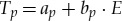. At a given temperature level (T_target) this implies that cumulative emissions for the target temperature level at the same probability level are 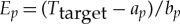. Calculating regression coefficients a_p and b_p for many probability levels (in this study we use percentiles) thus allows estimation of a probability distribution of carbon budget. Note this this is not a multiple linear regression as linearity is only assumed in the relation between warming and cumulative emissions, but not in the relation between probability level and cumulative emissions.

Since our focus is on the 2100 warming an alternative approach is also examined using a regression of warming onto cumulative emission estimates based only on 2100 values for each scenario. For lower temperature levels, this tends to produce smaller carbon budgets but larger changes in the budgets for the temperature perturbations caused by the extra Earth system feedback. However, we focus on the approach of using the entire time-series because more information is used in the regression and it gives a more conservative estimate of the carbon budget perturbation caused by the extra feedbacks.

3. Impact on the magnitude of warming and the time to exceed 1.5°C and 2°C

Our first set of simulations look at the temperature response to two future scenarios, RCP2.6 and RCP8.5. These are, respectively, the lowest and highest RCP forcing scenarios considered by AR5 and in terms of their implied emissions correspond to scenarios of either aggressive mitigation or a continuing increase in emissions. Figure 3 shows the probability of different levels of warming for the two scenarios at year 2100 with (shaded bands) and without (solid line) the contribution from additional Earth system feedbacks. The values from using a median estimate of the extra feedbacks are shown by the dashed lines. Figure 4 shows the variation of the probability of exceeding 1.5°C or 2°C over the course of the twenty-first century in the RCP2.6 simulation. In these figures, and throughout all other calculations in this study, temperature projections are relative to the 1850–1900 mean assuming that the median estimate of the mean 1986–2005 warming was 0.61°C, in line with the approach of IPCC [8].

Figure 3.

Cumulative probability of the warming being below a given temperature level at 2100 in RCP2.6 and RCP8.5 when no additional Earth system feedbacks are added (solid lines), and when our 5th to 95th percentile range of feedbacks are included (shaded region). (Online version in colour.)

Figure 4.

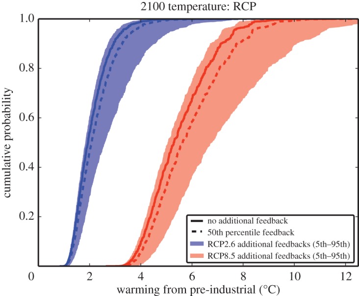
Evolution over time of the probability of the warming being below a given temperature level in RCP2.6 for 1.5°C and 2°C levels when no additional Earth system feedbacks are added (solid lines), and when our 5th to 95th percentile range of feedbacks are included (shaded regions). (Online version in colour.)

As expected, the impact on warming of the additional Earth system process is seen in figure 3 as ranging from a slight cooling effect from the 5th percentile of the distribution of extra feedbacks, to a potentially significant extra warming for the majority of the distribution of extra feedbacks. As the forcing distribution is skewed the difference between the 5th and 50th percentiles of extra feedbacks is less than that between the 95th and the 50th percentiles and this is reflected in the impact of the additional forcing on temperatures (figure 3). For a given scenario, the effects are largest for the model variants that would be expected to warm the most, with high transient climate response and strong climate-carbon cycle coupling. The size of the impact of the extra Earth system feedbacks on the higher emission and warmer scenario (RCP8.5) is considerably greater than on the low emission scenario (RCP2.6) and this is true for both the cooling and warming components of the shaded region. Care should be taken when considering the warmest model simulations as these may be well beyond the range of warming in the simulations used to derive the Earth system feedback strength.

A number of recent studies have focused on the time-scale of reaching particular levels of warming (see for instance [30]). Focusing on the probability of exceeding fixed warming levels above pre-industrial levels, even the lowest transient response versions of RCP8.5 are found to exceed 1.5°C and 2°C with a probability of more than 99% during the twenty-first century, it is simply a matter of when. When the additional Earth system feedback is negative this delays the timing of exceeding 1.5°C or 2°C of warming, but by a trivial amount of a year or less for the 5th percentile of extra feedbacks. When the additional Earth system feedbacks are positive the time of exceeding 1.5°C or 2°C is brought forward by a few years but still less than a decade for the case of the 1.5°C level and the 95th percentile of additional Earth system feedbacks.

The time-evolution of the probability of exceeding 1.5°C or 2°C levels is more interesting for the RCP2.6 scenario, because here, without additional feedbacks, there is already an appreciable chance of not exceeding these levels of global average warming during the twenty-first century. The probability that the temperature stays below 1.5°C and 2°C at all times during the twenty-first century is around 15% for 1.5°C and 50–60% for 2°C in the model set-up used here when no additional feedbacks are included (figure 4). This falls to around less than 10% and 30%, respectively, when the most extreme (95th percentile) estimate of the extra feedbacks is included. If we consider the date at which the median chance of staying under a warming level of 1.5°C is crossed (which is around model year 2030 when no extra feedbacks are included) then for the median estimate of the extra feedbacks the date is brought forward by around 3–5 years. For the 95th percentile estimate of forcing this date is brought forward by around a decade. The results for the 2°C threshold are similar but the impact on dates is slightly larger. This means that when considering the extra feedbacks, it is not just necessary to take account of the impact on levels of emission reduction and mitigation for a given warming limit, it is also necessary to consider the fact that warming happens sooner, which is relevant to adaptation. The slight increase in probability of staying below 1.5°C after 2050 is due to the more pronounced temperature overshoot in the 1.5°C case.

It is important to note that we are not providing a best estimate here of the year where the probability of limiting warming falls below a given level. Our simple climate model approach does not sample natural internal variability and is not able to replicate the observed warming slowdown during the 2000s. Instead, the purpose is to illustrate the change in the timing resulting from including the additional feedbacks. The supplementary material contains time series of global mean temperature for simulations with and without additional Earth system feedback for the four RCPs.

4. Impact of additional Earth system feedbacks on global cumulative carbon budgets

The main purpose of our study is to estimate how additional Earth system feedbacks might affect the warming associated with a given magnitude of cumulative CO₂ emissions. Estimates of how a given magnitude of cumulative emissions correspond to a particular likelihood of limiting warming to either 1.5°C or 2°C above pre-industrial levels are shown in figure 5 (numerical values are also shown in table S1 of the electronic supplementary material with an additional warming level). The solid curve shows the uncertainty from the variation in transient climate response and carbon cycle uncertainty sampled. We can consider the vertical axis as a level of risk aversion. For some levels of risk aversion, the allowable budget for the 1.5°C limit case is negative, indicating that in the model world the cumulative emissions had already exceeded a level consistent with 1.5°C of warming above pre-industrial levels by model year 2011.

Figure 5.

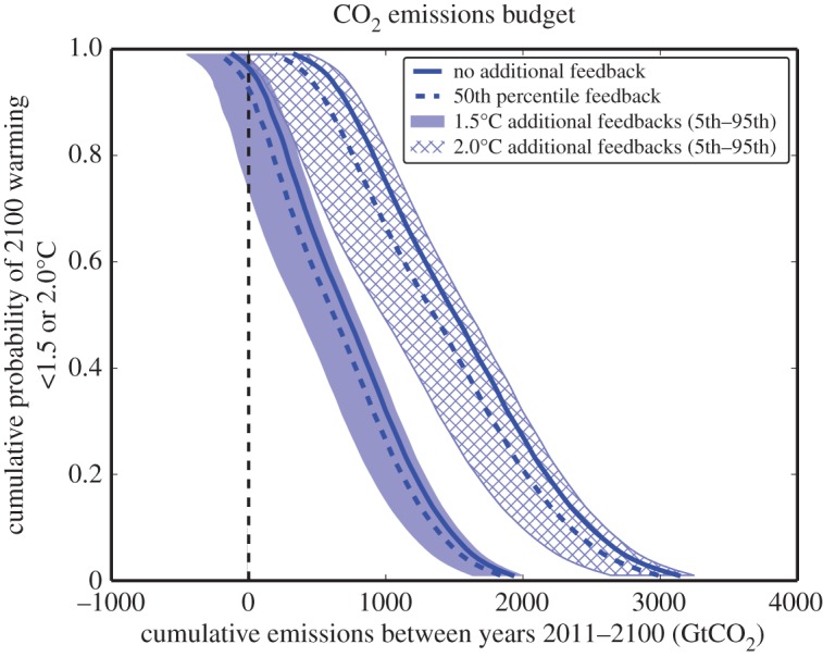
Estimated relationship between cumulative emissions and probability of staying below a given level of warming for 1.5°C (shaded) and 2°C (hatched), when no additional Earth system feedbacks are added (solid lines), and when our 5th to 95th percentile range of feedbacks are included (shaded region). (Online version in colour.)

Even without any additional Earth system feedbacks the size of the carbon budget for 1.5°C and 2°C varies considerably depending on the level of risk aversion. For the 1.5°C, this goes from a zero emission budget between 2011 and 2100 for around a 95% chance of staying below the warming limit, to around 720 GtCO₂ for a median chance. There is around a 100% chance of exceeding 1.5°C if the cumulative emissions of CO₂ exceed 2000 GtCO₂ during this period. The precise position and shape of the curve would be different had we used an alternative estimate of the uncertainty in transient climate response (or equilibrium climate sensitivity and ocean diffusivity), or a different carbon cycle-climate feedback. It is notable that our cumulative emissions budget estimate for median warming of 1.5°C without additional Earth system processes are somewhat larger than the IPCC synthesis report values, but are more similar to some other recent estimates [31]. For the 2°C case and similar levels of risk aversion the cumulative emissions are, as expected, larger.

The lowest estimates of our additional Earth system forcing tend to increase the allowable emissions by a small amount for the 1.5°C warming limit, although for the median case this is only by around 70 GtCO₂, or slightly less than 2 years of recent CO₂ emissions [32]. This reduces towards zero benefit for the largest budget with levels of risk aversion of just a few per cent chance of staying below 1.5°C (figure 5). This reflects the fact that TCRE is smaller for models at this end of the distribution so that a given change in warming corresponds to a lower change in implied CO₂ emissions than in the middle or upper tail of the distribution where TCRE values are larger.

The highest estimate of our additional Earth system forcing tends to decrease the allowable cumulative emissions for 1.5°C by around 350 GtCO₂ for a median risk aversion to warming. This perturbation to the allowable emissions is slightly smaller for the largest carbon budgets (low probabilities of limiting warming below the 1.5°C) and slightly larger for the lower carbon budgets (higher probability of limiting warming below 1.5°C).

Similar behaviour is seen for the 2°C warming limit case, but here the absolute values of the allowable carbon budget are somewhat larger. The perturbations to the allowable carbon budget from the extra Earth system feedbacks are also larger, with a reduction in the budget for a median probability of staying below 2°C of around 500 GtCO₂ for our 95th percentile of additional Earth system forcing.

5. Discussion

Our central result is that including additional Earth system feedbacks has the potential to make sizeable changes, and likely reductions, to the allowable global carbon budget corresponding to a given level of warming. To put these carbon budget changes in context we performed a number of sensitivity tests. In each case, we report the reduction in the allowable carbon emissions for the median chance of limiting warming to below 1.5°C. First, with no additional Earth system feedbacks included we tested two alternative distributions of the uncertainty in equilibrium climate sensitivity [33,34]. We then tested the sensitivity to the choice of deriving budgets from all RCPs, as done by default in this study, or just using RCP8.5 as done by IPCC WG1 [6]. Finally, we tested an alternative method for estimating the TCRE based on a fit to only the endpoint of the RCP simulations for each percentile. Figure 6 summarizes the tests with some numerical values also shown in table S1 of the electronic supplementary information).

Figure 6.

Impact on 2011–2100 cumulative allowable carbon emissions for a median chance of staying under the 1.5°C warming level for a range of sensitivity studies. The results indicate the change in size of the allowable carbon budget relative to our default case of 718 GtCO₂, with positive values indicating a larger budget and negative values a smaller or tighter budget. (Online version in colour.)

The biggest effect comes from the choice of the estimated distribution of equilibrium climate sensitivity, which for the distributions tested can either lead to a slight reduction in budget or a large expansion of the global allowable carbon budget. This illustrates why having a better estimate of the shape of the uncertainty distribution for climate sensitivity remains vital. The impact of using only RCP8.5 to determine budgets is to reduce allowable emissions because of the higher levels of forcing from non-CO₂ emissions in RCP8.5 compared to other RCPs. This effect is small for 3°C budgets where most model data in the TCRE regression is from RCP8.5, larger at 2°C where more data from RCPs 4.5 and 6.0 are included, and largest for the 1.5°C budgets where more data from the low non-CO₂ forcing RCP2.6 are included in the TCRE regression. Our study of Earth system feedbacks finds the effect on the carbon budget may be significant, but perhaps not as large as some of the other known uncertainties such as choice of ECS distribution. The final test based on using only 2100 data suggests the method of estimating the TCRE may also be important. We do not report the effect of combining these uncertainties but do highlight they are not independent. For instance our estimates of the effect of using only RCP8.5 data or the role of additional Earth system feedbacks would be expected to be altered by choosing an alternative equilibrium sensitivity distribution. We chose a distribution based on CMIP5 climate models because future progress in this area is likely to come from new Earth system model experiments with more of the missing Earth system processes included.

It is also useful to consider further one of the major assumptions used in our estimates, namely the use of published linear feedbacks for the additional Earth system processes. While new estimates of some individual Earth system forcing terms continue to emerge in the literature, we chose to use the values from the last IPCC assessment because it provides a synthesis of the literature. The studies from which the estimates of Earth system feedbacks were assessed typically use scenarios of increasing forcing with warming beyond the 1.5°C or 2°C. This raises the important question of whether the feedbacks can credibly be used for scenarios that have a sizeable chance of limiting twenty-first century warming to below 1.5°C or 2°C. We acknowledge that among the range of processes considered there is scope for either sub-linear or super-linear behaviour. Furthermore, there is evidence (e.g. [35]) of higher-order interactions between feedbacks although current confidence in these findings is low [7]. Since we are interested in the global total effect, large-scale spatial averaging may remove some of these local non-linear effects. Furthermore, taking the example of permafrost which is potentially the largest extra term we have included, other published work such as [36] and [18] follow a more process based approach to simulating permafrost loss and suggest that the contribution permafrost thawing makes to extra warming will vary fairly linearly with temperature, at least for small temperature perturbations.

We can also perform further quantitative tests, again focusing on the permafrost term and estimating where two recent studies of including the effect of permafrost thawing using process-based approaches sit within our distribution of results when we rerun our experiments for this single additional feedback type. Burke et al. [11] estimate for a scenario with strong mitigation that permafrost thawing might add up to 9% additional global warming by 2100. When we reran our set-up with only the permafrost term included in the extra Earth system feedbacks, we found the median 2100 warming estimate for RCP2.6 increased by 11% with the median estimate of permafrost feedback strength included. Thus, our median estimates appear broadly consistent with [11] despite the methodological differences. We can also make a comparison for the permafrost term with recent estimates of its effects on carbon budgets by [10]. They estimate a difference in their 2°C carbon budget from pre-industrial times (focusing on the non-overshooting case) due to including permafrost carbon in CO₂-only simulations to be around 105 GtC, or 380 GtCO₂. We find the reduction in the median estimate of our carbon budget for 2°C due to the permafrost term alone on the 2011 to 2100 budget, in similar CO₂-only simulations, to be 335 GtCO₂ for our median estimate of permafrost feedback. This comparison has to be used with care since some, although probably a small component, of the budget difference from including permafrost thawing in [10] may be accumulated before 2011. Again, there is an approximate agreement between our results and those of more detailed process studies.

Thus, we believe that despite its simplicity our approach provides a useful first attempt at illustrating the potential effects from a wide range of uncertain Earth system processes that so far have not been evaluated in terms of their combined impact on future warming or carbon budgets. We eagerly await the next generation of Earth system models where many of the Earth system processes missing during the last IPCC assessment might be included. Furthermore, work on emergent constraints might also allow us to constrain some of these processes further, and demonstrates the value of having both climate and Earth system observations.

6. Conclusion

In this study, we made estimates of the combined extra radiative feedbacks from additional Earth system processes. Our approach was first to construct an uncertainty distribution of the extra feedbacks, which was found to have a large probability of extra positive forcing (which would enhance planetary warming) but retained a small probability of negative forcing (which would offset planetary warming). This distribution of additional forcing was then applied within a simple climate model of the type often used in policy relevant studies of global warming for a given emission pathway. The effects were then investigated in terms of a perturbation to warming for a low- and high-emission scenario, and a perturbation to the twenty-first century cumulative carbon dioxide emissions (the carbon budget) compatible with staying below a given warming above pre-industrial levels.

Our study does not aim to produce a new best estimate of allowable carbon budgets, it instead seeks to highlight the potential uncertainty in budget estimates. The main findings of the study were that including Earth system feedbacks that are typically omitted from studies of allowable carbon budgets has a high probability of leading to more warming for a given scenario of anthropogenic emissions. It is also expected to lower the allowable cumulative carbon budget for the twenty-first century for a 1.5°C and 2°C warming limit. In the case of our upper estimate of the extra Earth system forcings, this corresponds to around a 350 GtCO₂ budget reduction for a 1.5°C limit and around a 500 GtCO₂ reduction for 2°C. When using median estimates for the extra Earth system forcing the budget reductions are around 100 GtCO₂ and 150 GtCO₂, respectively, for the two warming limits. Thus, the uncertainty in Earth system feedbacks on allowable carbon budgets is comparable with but not the largest of other remaining first-order uncertainties, such as the choice of uncertainty distribution of climate sensitivity.

While these large uncertainties remain we recommend that studies of mitigation feasibility and emissions reduction plans do not only focus on the current best central estimate of the allowable carbon budget, but also look at the upper and lower budget estimates. Just as flexible planning [37] is becoming more commonly used in adaptation there may be a need to follow similar approaches for mitigation. This would mean that while plans still initially focus on current best estimates of allowable carbon budgets, options are also developed and appraised that allow for lower allowable global budget estimates, or indeed higher estimates. Some research has already started to address this for the some of the deep uncertainties surrounding climate response (e.g. [29]), but this needs extending to include other budget uncertainties.

Data accessibility

The RCP emissions used in this study are available through the website (https://tntcat.iiasa.ac.at:8743/RcpDb/dsd?Action=htmlpage&page=welcome). The feedback distribution derived from the IPCC AR5 data and the model output are available from the authors on request.

Authors' contributions

J.A.L. and D.B. conceived the study. D.B. ran the simulations. D.B. and J.A.L. analysed and interpreted the results. J.A.L. and D.B. wrote the manuscript.

Competing interests

We declare we have no competing interests.

Funding

J.A.L. and D.B. were funded through the AVOID2 programme (DECC and Defra) under contract number 1104872 (www.avoid.uk.net). JAL and DB additionally acknowledge funding from the European Union Seventh Framework Programme (FP7/2007–2013) under grant agreement no. 265139 (AMPERE), where some of the initial thinking on this work was developed and an early version of the calculations performed.

References

- 1.Allen MR, Frame DJ, Huntingford C, Jones CD, Lowe JA, Meinshausen M, Meinshausen N. 2009. Warming caused by cumulative carbon emissions towards the trillionth tonne. Nature 458, 1163–1166. ( 10.1038/nature08019) [DOI] [PubMed] [Google Scholar]
- 2.Meinshausen M, Meinshausen N, Hare W, Raper SCB, Frieler K, Knutti R, Frame DJ, Allen MR. 2009. Greenhouse-gas emission targets for limiting global warming to 2 degrees C. Nature 458, 1158–1162. ( 10.1038/nature08017) [DOI] [PubMed] [Google Scholar]
- 3.Matthews HD, Gillett NP, Stott PA, Zickfeld K. 2009. The proportionality of global warming to cumulative carbon emissions. Nature 459, 829–832. ( 10.1038/nature08047) [DOI] [PubMed] [Google Scholar]
- 4.Gillett NP, Arora VK, Matthews HD, Allen MR. 2013. Constraining the ratio of global warming to cumulative CO2 emissions using CMIP5 simulations. J. Clim. 26, 6844–6858. ( 10.1175/JCLI-D-12-00476.1) [DOI] [Google Scholar]
- 5.Smith SM, Lowe JA, Bowerman NHA, Gohar LK, Huntingford C, Allen MR. 2012. The equivalence of greenhouse-gas emissions for peak temperature limits. Nat. Clim. Change 2, 535–538. ( 10.1038/nclimate1496) [DOI] [Google Scholar]
- 6.IPCC. 2014. Climate change 2014: synthesis report. In Contribution of Working Groups I, II and III to the Fifth Assessment Report of the Intergovernmental Panel on Climate Change (eds Core Writing Team, Pachauri RK, Meyer LA), 151 pp Geneva, Switzerland: IPCC. [Google Scholar]
- 7.IPCC. 2013. Climate change 2013: the physical science basis. In Contribution of Working Group I to the Fifth Assessment Report of the Intergovernmental Panel on Climate Change (eds Stocker TF, et al.), 1535 pp Cambridge, UK: Cambridge University Press. [Google Scholar]
- 8.IPCC. 2014. Climate change 2014: mitigation of climate change. In Contribution of Working Group III to the Fifth Assessment Report of the Intergovernmental Panel on Climate Change (eds Edenhofer O, et al.), 1435 pp. Cambridge, UK: Cambridge University Press. [Google Scholar]
- 9.Rogelj J, Schaeffer M, Friedlingstein P, Gillet NP, van Vuuren D, Riahi K, Allen M, Knutti R. 2016. Differences between carbon budgets unravelled. Nat. Clim. Change 6, 245–252. ( 10.1038/nclimate2868) [DOI] [Google Scholar]
- 10.MacDougall AH, Zickfeld K, Knutti R, Matthews HD. 2015. Sensitivity of carbon budgets to permafrost carbon feedbacks and non-CO2 forcings. Environ. Res. Lett. 10, 125003 ( 10.1088/1748-9326/10/12/125003) [DOI] [Google Scholar]
- 11.Burke EJ, Ekici A, Huang Y, Chadburn SE, Huntingford C, Ciais P, Friedlingstein P, Peng SS, Krinner G. 2017. Quantifying uncertainties of permafrost carbon-climate feedbacks. Biogeosciences 14, 3051–3066. ( 10.5194/bg-14-3051-2017) [DOI] [Google Scholar]
- 12.Burke E, Chadburn S, Huntingford C, Jones C. 2017. CO2 loss by permafrost thawing implies additional emissions reductions to limit warming to 1.5 or 2°C. Environ. Res. Lett. 13, 024024 ( 10.1088/1748-9326/aaa138) [DOI] [Google Scholar]
- 13.Landry JS, Matthews HD. 2017. The global pyrogenic carbon cycle and its impact on the level of atmospheric CO2 over past and future centuries. Global Change Biol. 23, 3205–3218. ( 10.1111/gcb.13603) [DOI] [PubMed] [Google Scholar]
- 14.Tesdal JE, Christian JR, Monahan AH, von Salzen K. 2016. Sensitivity of modelled sulfate aerosol and its radiative effect on climate to ocean DMS concentration and air-sea flux. Atmos. Chem. Phys. 16, 10 847–10 864. ( 10.5194/acp-16-10847-2016) [DOI] [Google Scholar]
- 15.Arneth A, et al. 2010. Terrestrial biogeochemical feedbacks in the climate system. Nat. Geosci. 3, 525–532. ( 10.1038/ngeo905) [DOI] [Google Scholar]
- 16.Friedlingstein P, et al. 2006. Climate-carbon cycle feedback analysis: Results from the C4MIP model intercomparison. J. Clim. 19, 3337–3353. ( 10.1175/JCLI3800.1) [DOI] [Google Scholar]
- 17.Collins WJ, et al. 2011. Development and evaluation of an Earth-System model— HadGEM2. Geosci. Model Dev. 4, 1051–1075. ( 10.5194/gmd-4-1051-2011) [DOI] [Google Scholar]
- 18.Burke EJ, Jones CD, Koven CD. 2013. Estimating the permafrost-carbon climate response in the CMIP5 climate models using a simplified approach. J. Clim. 26, 4897–4909. ( 10.1175/JCLI-D-12-00550.1) [DOI] [Google Scholar]
- 19.Schneider von Deimling TS, Meinshausen M, Levermann A, Huber V, Frieler K, Lawrence DM, Brovkin V. 2012. Estimating the near-surface permafrost carbon feedback on global warming. Biogeosciences 9, 649–665. ( 10.5194/bg-9-649-2012) [DOI] [Google Scholar]
- 20.Stocker BD, Roth R, Joos F, Spahni R, Steinacher M, Zaehle S, Bouwman L, Xu-Ri, Prentice IC.. 2013. Multiple greenhouse gas feedbacks from the land biosphere under future climate change scenario. Nat. Clim. Change 3, 666–672. ( 10.1038/nclimate1864) [DOI] [Google Scholar]
- 21.Stevenson DS, et al. 2006. Multimodel ensemble simulations of present-day and near-future tropospheric ozone. J. Geophys. Res. 111, D08301 ( 10.1029/2005JD006338) [DOI] [Google Scholar]
- 22.Gregory JM, Jones CD, Cadule P, Friedlingstein P. 2006. Quantifying carbon cycle feedbacks. J. Clim. 22, 5232–5250. ( 10.1175/2009JCLI2949.1) [DOI] [Google Scholar]
- 23.Wigley TML. 1993. Balancing the carbon budget—implications for projections of future carbon-dioxide concentration changes. Tellus Ser. B 45, 409–425. ( 10.1034/j.1600-0889.1993.t01-4-00002.x) [DOI] [Google Scholar]
- 24.Wigley TM, Raper SCB. 2001. Interpretation of high projections for global-mean warming. Science 293, 451–454. ( 10.1126/science.1061604) [DOI] [PubMed] [Google Scholar]
- 25.Lowe J, Huntingford C, Raper S, Jones C, Liddicoat S, Gohar L. 2009. How difficult is it to recover from dangerous levels of global warming? Envi. Res. Lett. 4, 014012 ( 10.1088/1748-9326/4/1/014012) [DOI] [Google Scholar]
- 26.IPCC. 2007. Contribution of the Working Group I to the Fourth Assessment Report of the Intergovernmental Panel on Climate Change (eds Solomon S, Qin M, Manning M, Chen Z, Marquis M, Averyt KB, Tignor M, Miller HL). Cambridge, UK: Cambridge University Press. [Google Scholar]
- 27.Forster PM, Andrews T, Good P, Gregory JM, Jackson LS, Zelinka M. 2013. Evaluating adjusted forcing and model spread for historical and future scenarios in the CMIP5 generation of climate models. J. Geophys. Res. 118, 1139–1150. ( 10.1002/jgrd.50174) [DOI] [Google Scholar]
- 28.Moss RH, et al. 2010. The next generation of scenarios for climate change research and assessment. Nature 463, 747–756. ( 10.1038/nature08823) [DOI] [PubMed] [Google Scholar]
- 29.Joshi M, Hawkins E, Sutton R, Lowe J, Frame D. 2011. Projections of when temperature change will exceed 2 degrees C above pre-industrial levels. Nat. Clim. Change 1, 407–412. ( 10.1038/NCLIMATE1261) [DOI] [Google Scholar]
- 30.Millar R. J., et al. 2017. Emission budgets and pathways consistent with limiting warming to 1.5°C. Nat. Geosci. 10, 741–747. ( 10.1038/ngeo3031) [DOI] [Google Scholar]
- 31.Le Quéré C, et al. 2016. Global carbon budget 2016. Earth Syst. Sci. Data 8, 605–649. ( 10.5194/essd-8-605-2016) [DOI] [Google Scholar]
- 32.Aldrin M, Holden M, Guttorp P, Skeie RB, Myhre G, Berntsen TK. 2012. Bayesian estimation of climate sensitivity based on a simple climate model fitted to observations of hemispheric temperatures and global ocean heat content. Environmetrics 23, 253–271. ( 10.1002/env.2140) [DOI] [Google Scholar]
- 33.Sexton DMH, Murphy JM, Collins M, Webb ML. 2012. Multivariate probabilistic projections using imperfect climate models part I: outline of methodology. Clim. Dyn. 38, 2513–2542. ( 10.1007/s00382-011-1208-9) [DOI] [Google Scholar]
- 34.Leuzinger S, Luo YQ, Beier C, Dieleman W, Vicca S, Körner C. 2011. Do global change experiments overestimate impacts on terrestrial ecosystems? Trends Ecol. Evol. 26, 236–241. ( 10.1016/j.tree.2011.02.011) [DOI] [PubMed] [Google Scholar]
- 35.Burke EJ, Hartley IP, Jones CD. 2012. Uncertainties in the global temperature change caused by carbon release from permafrost thawing. Cryosphere 6, 1063–1076. ( 10.5194/tc-6-1063-2012) [DOI] [Google Scholar]
- 36.Ranger N, Reeder T, Lowe JA. 2013. Addressing ‘deep’ uncertainty over long-term climate in major infrastructure projects: four innovations of the Thames Estuary 2100 Project. EURO J. Decis. Processes 1, 3–40. ( 10.1007/s40070-013-0014-5) [DOI] [Google Scholar]
- 37.Jarvis A, Leedal D, James Taylor C, Young P. 2009. Stabilizing global mean surface temperature: a feedback control perspective. Environ. Modell. Software 24, 665–674. ( 10.1016/j.envsoft.2008.10.016) [DOI] [Google Scholar]
Associated Data
This section collects any data citations, data availability statements, or supplementary materials included in this article.
Supplementary Materials
Data Availability Statement