Dynamic functional connectivity impairments in early schizophrenia and clinical high-risk for psychosis

Abstract

Individuals at clinical high-risk (CHR) for psychosis are characterized by attenuated psychotic symptoms. Only a minority of CHR individuals convert to full-blown psychosis. Therefore, there is a strong interest in identifying neurobiological abnormalities underlying the psychosis risk syndrome. Dynamic functional connectivity (DFC) captures time-varying connectivity over short time scales, and has the potential to reveal complex brain functional organization. Based on resting-state functional magnetic resonance imaging (fMRI) data from 70 healthy controls (HCs), 53 CHR individuals, and 58 early illness schizophrenia (ESZ) patients, we applied a novel group information guided ICA (GIG-ICA) to estimate inherent connectivity states from DFC, and then investigated group differences. We found that ESZ patients showed more aberrant connectivities and greater alterations than CHR individuals. Results also suggested that disease-related connectivity states occurred in CHR and ESZ groups. Regarding the dominant state with the highest contribution to dynamic connectivity, ESZ patients exhibited greater impairments than CHR individuals primarily in the cerebellum, frontal cortex, thalamus and temporal cortex, while CHR and ESZ populations shared common aberrances mainly in the supplementary motor area, parahippocampal gyrus and postcentral cortex. CHR-specific changes were also found in the connections between the superior frontal gyrus and calcarine cortex in the dominant state. Our findings show that CHR individuals generally show an intermediate functional connectivity pattern between HCs and SZ patients but also have unique connectivity alterations.

1. Introduction

In many patients with schizophrenia, a prodromal phase is evident before the onset of the full syndrome, characterized by attenuated psychotic symptoms and deterioration in functioning. Clinical criteria have been developed to identify individuals exhibiting these putatively prodromal symptoms (Klosterkotter et al., 2001; Miller et al., 2003; Yung et al., 2005), and individuals meeting these criteria have been shown to be at clinical high risk (CHR) for development of a full-blown psychotic disorder (Cannon et al., 2008; Fusar-Poli et al., 2012). Among CHR individuals, a subset (about 35%) converts to full-blown psychosis within 2.5 years of initial recruitment into longitudinal study protocols (Cannon et al., 2008; Fusar-Poli et al., 2012). CHR individuals are generally in some clinical distress and help-seeking, underscoring the fact that they are currently symptomatic and not simply at risk for future psychosis. The neural substrates associated with the CHR syndrome are just beginning to be characterized, and research efforts are underway (Borgwardt et al., 2013; Cannon et al., 2008; Fusar-Poli et al., 2012; Yung et al., 2003) to elucidate brain abnormalities underlying this syndrome as well as to improve identification of which CHR individuals will later develop a psychotic disorder.

There has been research using structural and functional imaging data (Dutt et al., 2015; Jung et al., 2010; Smieskova et al., 2013) to study CHR individuals. Both task-based and resting-state functional magnetic resonance imaging (fMRI) data have been employed to investigate functional activation and connectivity in CHR individuals (Anticevic et al., 2015; Fryer et al., 2013; Fusar-Poli et al., 2011; Jung et al., 2012; Morey et al., 2005; Pauly et al., 2010; Schmidt et al., 2013; Shim et al., 2010; Wang et al., 2016; Yoon et al., 2015). Reported differences using fMRI in CHR individuals, relative to healthy controls (HCs), have mainly involved the prefrontal, temporal, anterior cingulate and cerebellar regions that also showed abnormalities in patients with first episode psychosis (Fryer et al., 2013; Jung et al., 2012; Morey et al., 2005; Yoon et al., 2015). Functional connectivity (FC) derived from resting-state fMRI reflects the functionally integrated relationship between spatially separated brain regions, and may provide biomarkers for mental disorders (Bassett and Bullmore, 2009; Calhoun and Adali, 2012; Sporns, 2014; van den Heuvel and Hulshoff Pol, 2010; Zhang and Raichle, 2010). Most previous FC studies including CHR individuals (Anticevic et al., 2015; Jung et al., 2012; Shim et al., 2010; Wang et al., 2016; Yoon et al., 2015) have investigated networks seeded from a priori defined regions of interest (ROIs) (e.g., thalamus (Anticevic et al., 2015), superior temporal gyrus (Yoon et al., 2015), posterior cingulate cortex (Shim et al., 2010) and cerebellum (Wang et al., 2016)) by computing connectivity between a specific ROI and other voxels in whole brain. To our knowledge, no prior work has investigated whole-brain pair-wise FCs in CHR individuals using resting-state fMRI data. Moreover, the above mentioned research employed static FC (SFC) analyses, which assume that FC is unchanging across the scan acquisition period. However, recent studies have provided evidence that FC can be time-varying over periods of tens of seconds, evident during a few minutes of scans (Allen et al., 2014; Calhoun et al., 2014; Di and Biswal, 2015; Hutchison et al., 2013). Here we report the first study to examine whole-brain dynamic FC (DFC) in CHR individuals and patients in the early stages of schizophrenia using resting-state fMRI data.

DFC can be captured using a sliding time-window method (Hutchison et al., 2013). Different connectivity states, reflecting specific configurations of connected regions, can be revealed by post-hoc analyses of DFC (Calhoun et al., 2014; Damaraju et al., 2014; Du et al., 2017; Du et al., 2015; Du et al., 2016; Rashid et al., 2014; Yu et al., 2015), so alterations in connectivity states among different clinical populations might provide unique or additional biomarkers of disorders not detectable with SFC measures. There has been considerable work using DFC analyses to investigate impairments in schizophrenia-spectrum disorders and mood disorders (Damaraju et al., 2014; Du et al., 2017; Du et al., 2016; Rashid et al., 2014) as well as classifying individual patients based on DFC measures (Rashid et al., 2016). Researchers have applied clustering (Allen et al., 2014; Du et al., 2016), principal components analysis (PCA) (Leonardi et al., 2013), Fisher discrimination dictionary learning (FDDL) (Li et al., 2014), and spatial and temporal independent components analysis (ICA) (Miller et al., 2016; Yaesoubi et al., 2015) to extract connectivity states. These methods typically estimate connectivity states with discrepant patterns due to their different assumptions (Calhoun et al., 2014). Clustering approaches may fail to converge when working on “noisy” data that do not necessarily have desirable distributions. A more serious shortcoming of clustering is that the method always can yield a partition with any given number of clusters, regardless if the used features show patterns indicating clusters. Most previous decomposition-based work (Leonardi et al., 2013; Li et al., 2014; Miller et al., 2016; Yaesoubi et al., 2015) has focused on group-level connectivity states that are common across subjects.

To overcome some of the methodological limitations of the traditional DFC approaches, we have developed a novel group information guided ICA (GIG-ICA) (Du and Fan, 2013; Du et al., 2017; Du et al., 2015) framework to analyze DFC. Guided by the group-level connectivity states, our method can extract the subject-specific connectivity states using a multiple-objective optimization framework. The subject-specific states are directly comparable across subjects, which benefits the exploration of disease biomarkers. In our previous work (Du et al., 2017) using the proposed method, we detected group differences among a spectrum of symptomatically-related disorders including bipolar disorder with psychosis, schizoaffective disorder and schizophrenia, suggesting that our dynamic connectivity analysis method is able to identify potential biomarkers that were not evident using the conventional static connectivity analysis. Both hypo-connectivities and hyper-connectivities were observed for those diagnoses, and interestingly the connections’ strengths had reasonable associations with the symptom scores. In the present study, we applied the method to the resting-state fMRI data of HCs, CHR individuals and early illness schizophrenia (ESZ) patients, aiming to find DFC characteristics that differentiate these groups. We hypothesized that CHR subjects would share several of DFC alterations apparent in ESZ, but would show intermediate changes between the HC and ESZ groups.

2. Materials and methods

2.1. Materials

Resting-state fMRI data from 70 HCs, 53 CHR individuals, and 58 ESZ patients were analyzed. Table 1 shows the demographic and clinical information. There are no significant differences among the three groups on age or gender (p-value = 0.7 for gender examined by Chi Square test; p-value = 0.2 for age examined by analysis of variance). CHR individuals were recruited from the University of California, San Francisco’s (UCSF) Prodromal Assessment, Research, and Treatment Clinic. Individuals recruited to the CHR group met the Criteria of Prodromal Syndromes (COPS) based on a Structured Interview for Prodromal Syndromes (SIPS) (Miller et al., 2003). The COPS comprises three non-mutually exclusive syndromes (McGlashan et al., 2010): Attenuated Positive Symptom Syndrome (APSS), Brief Intermittent Psychotic Syndrome (BIPS), and/or Genetic Risk and Deterioration Syndrome (GRD). The majority (92.5%) of CHR subjects met COPS criteria for APSS. Supplementary Table S1 shows the number and percentage of CHR subjects with each syndrome. Clinical ratings of symptom severity in CHR individuals were obtained using the Scale of Prodromal Symptoms (SOPS), an embedded scale within the SIPS. Most of the CHR subjects (41/53; 77%) were antipsychotic medication-naive at the time of scanning. ESZ patients within mean ± standard deviation = 2.08 ± 1.37 years of illness onset were recruited from an early psychosis clinic at UCSF and from community clinics. Diagnosis of schizophrenia or schizoaffective disorder in ESZ participants was verified using the Structured Clinical Interview for DSM-IV (SCID) (Ventura et al., 1998), and symptom severity was assessed using the Positive and Negative Syndrome Scale (PANSS) (Kay et al., 1987). Most ESZ patients (53/58; 91%) were taking antipsychotic medication at the time of testing. HCs were recruited from the community and did not meet criteria for any Axis I diagnosis based on the SCID. Written informed consent was obtained from study participants under protocols approved by the Institutional Review Board at UCSF.

Table 1.

Subject and clinical characteristics.

	HCs (n=70)		CHR individuals (n=53)		ESZ patients (n=58)
	Mean	SD	Mean	SD	Mean	SD
Age (Years)	21.9	5.6	20.4	4.5	21.8	3.8
PANSS Positive Symptoms	–	–	–	–	13.7	4.8
PANSS Negative Symptoms	–	–	–	–	17.4	6.6
PANSS General Symptoms	–	–	–	–	32.9	8.9
SOPS Positive Symptoms	–	–	9.4	4.5	–	–
SOPS Negative Symptoms	–	–	12.2	5.8	–	–
SOPS General Symptoms	–	–	8.1	4.5	–	–
SOPS Disorganization Symptoms	–	–	5.4	3.4	–	–
Maximum translation motion displacement (mm)	0.8	0.6	1.1	1.4	1.2	1.3
Maximum rotation motion displacement (degree)	0.8	1.0	1.0	0.9	0.9	0.8
	n	%	n	%	n	%
Male	41	59%	32	62%	38	65%

SD, standard deviation; HCs, healthy controls; CHR, clinical high-risk; ESZ, early illness schizophrenia; PANSS, Positive and Negative Syndrome Scale; SOPS, Scale of Prodromal Symptoms. The maximum translation motion displacement was computed as the maximum translation across all axes (x-axis, y-axis and z-axis) and the whole scanning. The maximum rotation motion displacement was computed as the maximum rotation across the pitch, roll and yaw and the whole scanning.

All brain images were acquired on a 3T TIM TRIO scanner at the UCSF Neuroimaging Center. Resting-state scans were acquired using high-speed whole-brain echo-planar imaging (EPI) sequences. Rest scans lasted six minutes, during which 180 functional images were obtained (32 axial slices, 3.5 mm slice thickness, 1.05 mm inter-slice gap, TR = 2 s, TE = 29 ms, flip angle = 75°, FOV = 24 cm, 64 × 64 matrix). Participants were instructed to rest with eyes closed and stay awake.

FMRI data of each subject were preprocessed using the Data Processing Assistant for Resting-State fMRI (DPARSF) toolbox (Yan and Zang, 2010) based on Statistical Parametric Mapping (SPM8) (http://www.fil.ion.ucl.ac.uk/spm). The first 10 volumes were discarded, and then the remaining images were slice-time corrected and realigned for head-motion correction. For each subject, the translation of head motion was less than 4 mm and the rotation of head motion did not exceed 4 degrees in all axes through the whole scanning process. The mean and standard deviation of the summarized head motion measures across subjects are reported for each group in Table 1. Analysis of variance (p < 0.05) showed no significant group difference in either the maximum translation motion displacement or the maximum rotation motion displacement. Subsequently, the images were spatially normalized to the Montreal Neurological Institute (MNI) EPI template, resliced to 3 mm × 3 mm × 3 mm voxels, and smoothed with a Gaussian kernel with a full-width at half-maximum (FWHM) of 6 mm. Detrending and band-pass filtering (0.01Hz–0.08Hz) (Auer, 2008; Cordes et al., 2001; Zuo et al., 2010) were then performed to remove higher frequency physiological noise and lower frequency scanner drift. Finally, nuisance covariates including six head motion parameters, white matter signal, cerebrospinal fluid signal, and global mean signal (Fox et al., 2005) were regressed out, and then residual images were saved for subsequent analyses. Note: the white matter signal, cerebrospinal fluid signal and global mean signal used as covariates were obtained after the detrending and band-pass filtering processing.

2.2. Methods

Firstly, time-varying functional connectivity was estimated using a sliding time-window method, and then inherent connectivity states can be computed using our proposed decomposition-based method. The overall framework of estimating dynamic connectivity and connectivity states is shown in Fig. 1. Detailed procedures are explained in the following subsections. Finally, we investigated group differences based on the individual-subject’s connectivity states, aiming to reveal potential biomarkers.

Fig. 1.

The schematic drawing of analysis steps. A: Estimation of dynamic functional connectivity (DFC) of individual subject (e.g., the kth subject) using a sliding time-window method based on regions of interests (ROIs). For each subject, a window-by-connectivity matrix (e.g., X^k) is obtained to reflect its DFC. B: Computation of group-level connectivity states. For each group, the window direction-concatenated dynamic connectivity matrix X from all N subjects was decomposed by ICA to obtain M group-level states (GSs) and the subject-specific fluctuations (SFs) of these states. C: Computation of individual-subject’s connectivity states. Based on the dominant group-level state (i.e., S_l) and individual-subject’s dynamic functional connectivity matrix (e.g., X^k), the dominant subject-specific state (SS, e.g., $S_l^k$) of each subject can be computed.

2.2.1. Estimating dynamic functional connectivity

As shown in Fig. 1A, using the sliding time-window method, we computed whole-brain DFC for each subject based on 116 ROIs from the automated anatomical labeling (AAL) template (Tzourio-Mazoyer et al., 2002). The index (ID) and name of each ROI can be found in supplementary Table S2. For the averaged time-series within each ROI, we segmented it using a sliding time-window that was created by convolving a rectangle (width = 20 TRs) with a Gaussian (σ = 3 TRs) (Allen et al., 2014; Zalesky and Breakspear, 2015). The window length was 40 s (2 s × 20), which has extensively evaluated and shown to be suitable for capturing dynamics in FCs (Abrol et al., 2016; Allen et al., 2014; Damaraju et al., 2014; Zalesky and Breakspear, 2015). The window slid in steps of 1 TR, resulting in 151 short time-series for each ROI. Afterwards, regarding each window, a 116 × 116 connectivity matrix was calculated based on the associated short time-series of all ROIs (Allen et al., 2014; Damaraju et al., 2014). Each connectivity matrix reflecting the temporal correlations among ROIs within one window was estimated from a regularized inverse covariance matrix (Du et al., 2017; Smith et al., 2011) using a graphical LASSO framework (Friedman et al., 2008). LASSO imposed sparsity by placing an L1 norm penalty on the inverse covariance matrix to decrease noise effect of short time series. After obtaining the regularized inverse covariance matrix, its corresponding covariance matrix was calculated and then transformed into a correlation matrix, representing the functional connectivity matrix. Thus, for each subject, 151 connectivity matrices were obtained, reflecting time-varying functional connectivity between paired ROIs. Due to the symmetry of connectivity matrix within each window, the upper half 6670 unique elements can reflect connectivity strengths among 116 ROIs. Taking the kth subject for an example, its dynamic connectivity can be denoted by a window-by-connectivity matrix X^k (size: 151 × 6670). We then performed a r-to-z Fisher transformation on X^k.

2.2.2. Estimating functional connectivity states

Previous work (Allen et al., 2014; Calhoun et al., 2014; Du et al., 2017; Leonardi et al., 2013; Miller et al., 2016) has shown that multiple connectivity states exist in the time-varying connectivity. In the study, we sought to investigate whether HC, CHR and ESZ groups showed differences in the connectivity states; and if true, whether these changes showed a progressive trend from the healthy condition to psychosis risk to early schizophrenia. Our recently proposed dynamic connectivity analysis method (Du et al., 2017) was applied to estimate the connectivity states. In our method, the connectivity states are decoded by the independent components (ICs), and the loadings of ICs represent the fluctuations of connectivity states. Considering there are probably connectivity states with group-specific patterns among the three groups, we extracted connectivity states for each group. The following processing steps were implemented for each group separately.

We concatenated the window-by-connectivity matrices of all subjects along the window direction and obtained a matrix X= [X¹;…;X^k;…;X^N], (k = 1,…,N), where N was the number of subjects. As shown in Fig. 1B, we performed ICA (Amari et al., 1996; Bell and Sejnowski, 1995) using ICASSO technique (Ma et al., 2011) on the whole dynamic connectivity matrix (i.e., X) to compute the reliable group-level connectivity states (GSs). Before ICA, subject-level PCAs and a following group-level PCA (Erhardt et al., 2011) were used to reduce the dimensionality of the window direction. Thus, we had X = A·S, where S = [S₁;…; S_l;…;S_M] included all group-level ICs. S_l can represent information of the lth GS. Although it is hard to determine an optimal setting for the number of components, many prior studies (Damaraju et al., 2014; Du et al., 2017; Miller et al., 2016; Yaesoubi et al., 2015) suggested five connectivity states to estimate in dynamic connectivity analysis. So, consistent to previous work, M was set to 5 in this study. Using this setting, the mean of preserved variances was 76% in subject-level PCAs (Erhardt et al., 2011) and reliable performance of ICASSO with 20 ICA runs was achieved (see supplementary Fig. S1). Each GS (i.e., one row of S) was z-scored to zero mean and unit variance for consequent processing. According to ICA, A= [A¹;…;A^k;…;A^N] included the mixing coefficient matrices of all subjects. A^k represented the temporal fluctuations of all connectivity states for the kth subject, and each column of A^k reflected the subject-specific fluctuation (SF) of one state for the kth subject.

Afterwards, we assessed the contribution of each GS to the dynamic connectivity. The contribution of the lth GS was measured using $\mathit{sum}(\mathit{abs}(a_l))/{\displaystyle {\sum }_{l=1}^M\mathit{sum}(\mathit{abs}(a_l))}$, where a_l was the lth column of A. The measure reflected the percentage of the loading of each GS in all GSs’ loading sum. Consequently, the first-rank GS was identified as the dominant GS (e.g., S_l), which included the most information across entire dynamic connectivity stream of all subjects.

Subsequently, based on the identified dominant GS and the individual-subject’s Fisher-transformed dynamic connectivity matrix (e.g., X^k), we estimated the corresponding dominant subject-specific state (SS) using a multiple-objective function optimization (see the following formula (1)). Fig. 1C shows the schematic drawing of the step. In the procedure, the independence of the dominant SS as well as the correspondence between the dominant SS and the dominant GS were simultaneously optimized, resulting in accurate individual-level connectivity states that can be directly comparable across subjects. The optimization can directly yield Z-scored individual-level states with zero mean and unit variance.

$$\mathit{max}\{\begin{array}{c}J\left(S_l^k\right)={\left\{E\left[G\left(S_l^k\right)\right]-E\left[G\left(\nu \right)\right]\right\}}^2\\ F\left(S_l^k\right)=E[S_l{S}_l^k]\end{array}$$ (1)

$$s.t.\Vert w_l^k\Vert =1.$$

In (1), $S_l^k={(w_l^k)}^T·\stackrel{\sim }{X^k}$ represents the estimated dominant SS of the kth subject, where $\stackrel{\sim }{X^k}$ is the whitened X^k; $w_l^k$ is the unmixing column vector. The first function is for optimizing the independence measure of $S_l^k$. In our method, $J\left(S_l^k\right)$, the negentropy of $S_l^k$, is used to reflect independence of $S_l^k$. Here, ν is a is a Gaussian variable with zero mean and unit variance; G (·)is a nonquadratic function. The second function $F\left(S_l^k\right)$ is used to measure the similarity (i.e., correspondence) between S_l. and $S_l^k$. E[ ] denotes the expectation of variable. By derivation (Du and Fan, 2013), $E[S_l{S}_l^k]$ equals to Pearson correlation between S_l and $S_l^k$. To solve the multiple-objective function optimization, a linear weighted sum method was applied to combine the two objectives (Du and Fan, 2013). After the optimization, the dominant subject-specific states were obtained.

Derived from the above mentioned analyses, each of the group-level and individual-subject connectivity states is denoted by a Z-scored component (size: 1 × 6670). We then converted each component to a 116 × 116 symmetric matrix, so each element of the symmetric matrix reflects the relationship between one pair of ROIs. It is worth pointing out that the positive and negative values in the symmetric matrix of each GS should be interpreted along with the state’s loadings (i.e., SFs) due to the ambiguity of the signs of components (i.e., states). If one state’s SF values are positive, it means that its contribution to time-varying connectivity is positive. So, the positive/negative values in the state (i.e., the positive/negative values in the symmetric matrix) reflect the positive/negative connectivity strengths between ROIs. If one state’s SF values have both positive and negative values, the values in the symmetric matrix don’t directly correspond to the connectivity strengths. In that case, the positive (or negative) value in SF means that the state (or anti-state) exists in the corresponding window’s functional connectivity.

2.2.3. Investigating group differences in the functional connectivity states

In the section, we focus on investigating group differences in the connectivity states, aiming to explore whether CHR individuals tend to be intermediate between HC subjects and ESZ patients and what measures could be employed as potential biomarkers for CHR and ESZ.

Similar to our previous work (Du et al., 2017), we matched results among the three groups in order to compare the corresponding states. The detailed matching method is described in the supplementary materials. After that, we visualized each of GSs using the BrainNet Viewer toolbox (Xia et al., 2013) to reflect the related connectivity pattern among ROIs. Next, to assess the relationship (similarity or disparity) of the matched GSs across the three groups, we computed Pearson correlation coefficient between any pair of GSs, resulting in a correlation matrix (size: 3 × 3). The upper triangular elements of the correlation matrix include r_HC–CHR, r_HC–ESZ, and r_CHR–ESZ. Here, r_HC–CHR denotes the correlation between the GS of HC group and the GS of CHR group. Then, we took the mean of the absolute correlations in the similarity matrix as the overall similarity measure of the matched GSs.

Furthermore, we examined if the inter-group relationships of GSs are statistically significant using multiple permutation runs. For each group, we generated 100 permutations, each of which randomly included 85% samples of the original subjects. In each permutation run, the group-level ICA (shown in Fig. 1B) was applied to analyze the selected subjects’ dynamic connectivity, resulting in new GSs of the group. For each group, we then matched the new GSs from each permutation run with the GSs obtained from the original samples using a greedy search rule. So, the new GSs from each permutation run were re-sorted to provide correspondence across the three groups. Regarding each of 100 runs, a 3 × 3 correlation matrix associated with one state can be computed, representing the inter-group relationship of GSs in the run. Finally, for each state, we investigated if r_HC–CHR, r_HC–ESZ, and r_CHR–ESZ had significant differences by performing two-tailed two-sample t-tests between r_HC–CHR and r_HC–ESZ, between r_CHR–ESZ. and r_HC–CHR, as well as between r_CHR–ESZ and r_HR–ESZ based on the values from 100 permutation runs. Significant level was set to p < 0.01 with Bonferroni correction (i.e., p < 0.01/15).

Due to the importance of the dominant state (with the most contribution to the dynamic connectivity), we investigated its group differences in detail. First, we averaged the dominant SSs across subjects for each group to see if the connectivity patterns are disparate (or consistent) across groups. Then, analysis of covariance (ANCOVA) with age and gender as covariates was performed on each connection’s strengths in the dominant SSs to investigate the group difference of three groups. Afterwards, based on each connectivity showing group differences identified by ANCOVA (p < 0.05 with Bonferroni correction), we applied a two-tailed two-sample t-test (p < 0.05 with Bonferroni correction) to assess differences in connectivity strength between any pair of groups. Finally, for each connection with significant group difference, Pearson correlation coefficients between the connectivity strengths and symptom severity scores (shown in Table 1) were computed for the CHR and ESZ groups, respectively, in order to explore the associations between potential biomarkers and clinical symptoms. The correlation analyses were restricted to the subjects rated within a month of the scan session. The significance level was set to p < 0.05 (without correction) for correlation analyses.

In our work, the connectivity states were estimated from each group’s time-varying connectivity, separately. Since this strategy may raise concerns on whether the identified group differences were due to the grouping, we performed a permutation test (including 1000 permutation runs) to verify the effectiveness. Regarding each of 1000 permutations, we performed the following three steps. (1) We generated three dummy groups by randomly rearranging all subjects of the original three groups (i.e., HC, CHR and ESZ groups). Each of the dummy group had the same number of subjects with the original group. (2) Consistent with the processing on the original groups, we first estimated the group-level states by performing ICA on the dynamic connectivity of each dummy group, and then identified the dominant group-level state, finally computed the corresponding dominant subject-specific states. (3) We employed ANCOVA on each FC’s strengths of the dominant subject-specific states for the three dummy groups. While performing ANCOVA, the used age and gender information of each subject was the subject’s real information. After the 1000 permutation runs, we summarized the permutation test’s result by calculating the occurring frequency of the case where the p-value obtained from ANCOVA using rearranged groups (i.e., the dummy groups) was smaller than the corresponding p-value obtained from ANCOVA using the original (i.e., real) groups. The frequency (i.e., the tail probability computed from 1000 permutations) reflects the significance level of the identified group difference. Smaller tail probability corresponds to lower possibility of false positives of the identified group difference. (4) In order to identify FCs showing significant group differences in the permutation test, we further performed a step-down minP method proposed by Westfall & Young (Ge et al., 2003; Peter H. Westfall and Young, 1993) for multiple comparison corrections based on the p-values from 1000 permutations. After obtaining the adjusted p-values for all FCs, FCs with significant group differences can be identified.

3. Results

3.1. Group differences in the group-level functional connectivity states

After the state matching, the corresponding group-level connectivity states of the three groups are shown in the matrix form (size: 116 × 116) in Fig. 2. Together, we also display the rendered connectivity patterns of those states. As expected, the dominant GS had the highest contribution (49%, 45% and 47% for the HC, CHR and ESZ groups, respectively) to the dynamic connectivity, while each of the other four states’ contributions were around 10%. Similarity measures between the matched GSs were computed to investigate their relationship between the three groups. The similarity matrices shown in the last row of Fig. 2 indicate that the dominant GSs were very consistent across groups (similarity measure = 0.94), however, the remaining four GSs were discrepant (similarity measures = 0.64, 0.59, 0.55 and 0.44, respectively). Furthermore, the correlation matrices indicate that compared to the HC group, the CHR and ESZ groups had greater inter-group similarity in the non-dominant states, indicating that these states could be disease-related.

Fig. 2.

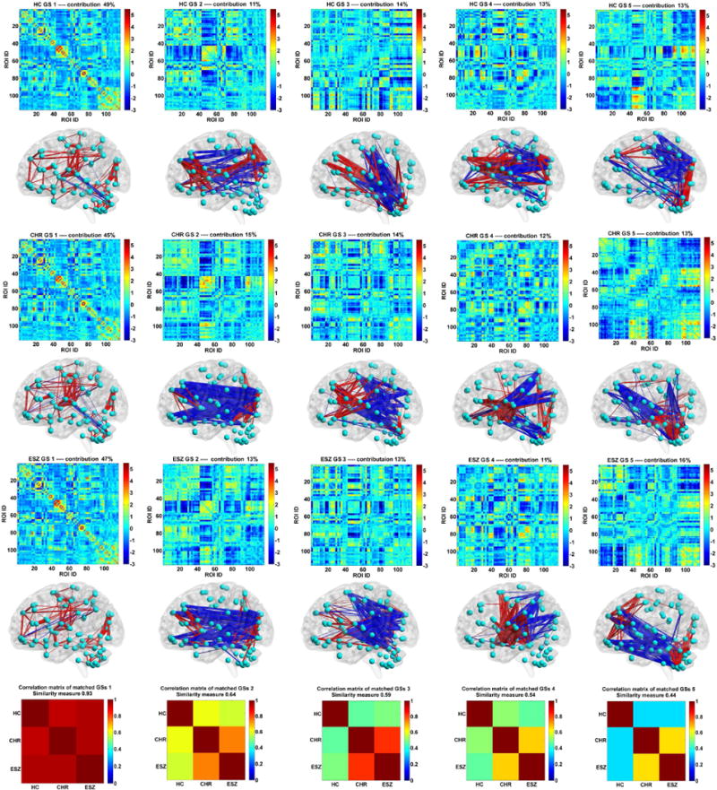
The corresponding group-level connectivity states (GSs) in matrix form, rendered form, and their inter-group correlations for healthy control (HC), clinical high-risk (CHR) and early illness schizophrenia (ESZ) groups. Each rendered GS is another view of the associated GS matrix, shown using the BrainNet Viewer toolbox with the same sparsity. The red and blue lines represent positive and negative values, respectively. The first column corresponds to the dominant GS. The last row shows the correlation matrix of three matched GSs from three groups. The overall similarity between the matched GSs is also shown along with each correlation matrix.

As mentioned in the method section, we further calculated GSs and their relationships across groups by implementing 100 permutation runs. Based on the correlation matrices associated with one state (e.g., GS 1) from 100 permutation runs, we averaged those matrices to yield a mean correlation matrix. Fig. 3 shows that each mean correlation matrix showed a quite similar pattern with that in Fig. 2. Also, we examined the differences in the inter-group similarity (e.g., the difference between r_CHR–ESZ and r_HC–CHR) of GSs by performing two-sample t-tests on the values from 100 runs. The statistical results are summarized in Table 2. The results support that there were no differences among r_CHR–ESZ, r_HC–CHR and r_HC–ESZ for GS 1. Regarding GS 2, GS 3, GS 4, and GS 5, both the difference between r_CHR–ESZ and r_HC–CHR and the difference between r_CHR–ESZ and r_HC–ESZ were statistically significant. The difference between r_HC–CHR and r_HC–ESZ was not significant for GS 2, GS 4 and GS 5, but significant for GS 3. The results suggest that CHR and ESZ groups showed more similarity in GS 2, GS 4 and GS 5 than any other pairs. GS 3 was different in all the three groups, while CHR and ESZ were relatively closer. The results support our above conclusion that the non-dominant states could be disease-related.

Fig. 3.

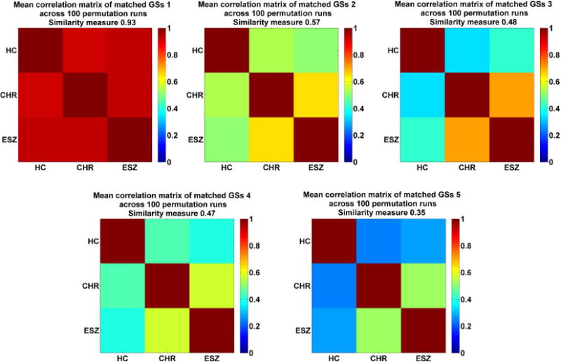
The mean correlation matrix of the matched GSs across 100 permutation runs for each state. The overall similarity between the matched GSs is also shown along with each correlation matrix.

Table 2.

The statistical results from the two-tailed two-sample t-tests that investigated the differences in similarity relationship of GSs based on the 100 permutation runs.

	GS 1	GS 2	GS 3	GS 4	GS 5
p-value of two-sample t-test between rHC–CHR and rHC–ESZ	0.008	0.096	3.040e–06	0.011	0.265
T-value of two-sample t-test between rHC–CHR and rHC–ESZ	−2.671	1.671	−4.805	2.571	−1.117
p-value of two-sample t-test between rCHR–ESZ and rHC–CHR	0.001	2.257e–16	1.253e–63	1.196e–06	2.493e–21
T-value of two-sample t-test between rCHR–ESZ and rHC–CHR	3.314	8.971	25.176	5.0111	10.684
p-value of two-sample t-test between rCHR–ESZ and rHC–ESZ	0.242	7.551e–21	5.632e–58	1.019e–16	9.893e–20
T-value of two-sample t-test between rCHR–ESZ and rHC–ESZ	1.173	10.521	23.055	9.094	10.141

For each state, the associated SFs across all windows of all subjects are demonstrated in Fig. 4. It illustrates that the dominant state had relatively higher values of SFs for most windows. Since the dominant state only had positive SFs (Fig. 4), the positive/negative values in the dominant state (i.e., the positive/negative values in the matrix of GS 1) reflected the positive/negative connectivity strengths between ROIs. For the dominant state, the positive connectivities (reflecting positive correlations among ROIs) primarily involved connections within the default mode network, the sensory-motor network, the vision-related network and within-cerebellum connections, while negative connectivities linking cerebellar crus and other cortices (including rolandic, insula, Heschl’s gyrus and superior temporal lobe). For each of the non-dominant states, both positive and negative values occurred in SFs (Fig. 4). Hence, the positive/negative values of the non-dominant states didn’t directly reflect the connectivity strengths.

Fig.4.

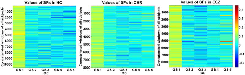
Values of subject-specific fluctuations (SFs) in the concatenated windows of all subjects for each state.

3.2. Group differences in the dominant subject-specific functional connectivity state

Regarding the dominant individual-level connectivity state of each subject, we averaged them in each group. The matrices and rendered view of the mean dominant SSs (Fig. 5A–C) show that the three groups showed a similar pattern in terms of the most important connectivity state, with the CHR group being intermediate between HC and ESZ groups. Furthermore, 30 FCs (see Fig. 5D and the supplementary Table 3) with significant group difference were identified by comparing the dominant SSs across the three groups using ANCOVA. Those aberrant connections mainly lay within cerebellum, between temporal cortex and cerebellum, between frontal cortex and thalamus, between supplementary motor area and parahippocampal gyrus, between supplementary motor area and temporal cortex, between postcentral and temporal cortex, between parahippocampal gyrus and temporal cortex, and between Hesch1’s gyrus and cerebellum.

Fig. 5.

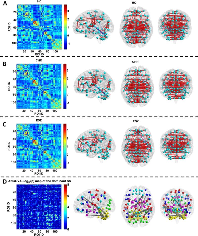
A–C: The functional connectivity matrix of the mean dominant subject-specific FC state (SS) across subjects and its visualized pattern for the healthy control (HC), clinical high-risk (CHR) and early illness schizophrenia (ESZ) group, respectively. In A–C, the red and blue lines represent the positive and negative strengths, respectively. D: Left: Statistical map (−log₁₀ (p) values) obtained by performing analysis of covariance (ANCOVA) with age and gender as covariates on each connection in the dominant SSs of three groups. Right: The visualized pattern of the 30 FCs showing significant group difference (p < 0.05 with Bonferroni correction, i.e., p < 0.05/6670). The thickness of the line reflecting one edge reflects the associated F-value. The colors of the nodes and edges in the subfigure D are organized by their modules in the AAL template provided by the BrainNet Viewer software. Nodes belonging to the same module and edges linking such nodes are shown using the same color. Edges linking two nodes belonging to different modules are shown in grey color.

Among the 30 FCs showing significant group difference, the mean connectivity strength of the CHR group fell in between the HC and ESZ groups for 25 FCs (see Fig. 6A), indicating that high risk stage tended to show an intermediate trend in connectivity between healthy condition and disease phase. Two-sample t-test results (Fig. 6A) further suggest that 16 FCs in the ESZ group showed significant alterations compared to both the HC and CHR groups, indicating that ESZ patients had greater connectivity abnormality than CHR individuals in these FCs. The 16 FCs were associated with the cerebellum, temporal cortex, frontal gyri, and thalamus. Furthermore, 12 FCs involving the supplementary motor area, parahippocampal gyrus, temporal cortex, postcentral gyrus, cerebellum, frontal gyri and thalamus were significantly different between the HC group and the other two groups, suggesting that the CHR and ESZ groups showing similar changes in these FCs. For the remaining two FCs linking the medial part of the superior frontal gyrus and calcarine cortex, the CHR group differed from both the HC and ESZ groups, reflecting a CHR-specific change. Therefore, our results generally show that the ESZ patients had the greatest number and most severe changes, while CHR individuals tended to fall intermediately between the ESZ and HC groups. Additionally, the CHR group exhibited a distinct FC alteration not evident in the ESZ group.

Fig. 6.

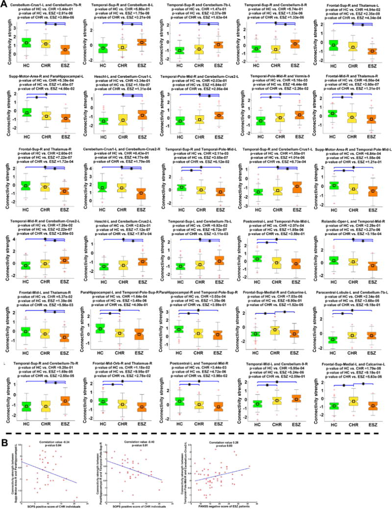
A: Two-sample t-test results of the identified 30 FCs in the dominant subject-specific FC state (SS). The result of each FC is shown in one sub-figure, the title of which denotes the associated two regions of interest (ROIs). For each of the 30 FCs, connectivity strengths of all subjects in one group are shown using one boxplot. Any pair of groups showing a significant difference (two-sample t-test, p < 0.05 with Bonferroni correction) is denoted using a blue line with a star (*) between them. P-values of two-sample t-tests (HC vs. CHR, HC vs. ESZ and CHR vs. ESZ) are also shown in the title. B: Significant correlations (with p < 0.05) between the FC strengths and the symptom scores for the clinical high-risk (CHR) or early illness schizophrenia (ESZ) group.

Several FCs’ strengths were associated with the symptom scores. The FC linking right supplementary motor area and left parahippocampal gyrus as well as the FC linking right parahippocampal gyrus and right temporal pole (superior temporal gyrus) showed a decreasing trend across HC, CHR and ESZ groups; meanwhile the two FCs were negatively correlated with SOPS positive symptom severity scores in the CHR group (Fig. 6B). The connection between right temporal pole (middle temporal gyrus) and left cerebellum exhibited increasing strength from the HC to the CHR to the ESZ groups, while its connectivity strength was positively correlated with PANSS negative symptom severity scores in the ESZ group (Fig. 6B). The results support the clinical relevance of the connectivity-based measures.

As described in section 2.2.3, we also performed a permutation test to examine the validity of the identified group differences. Fig. 7A shows all connections’ p-values obtained by performing ANCOVA on each connection’s strengths in the dominant subject-specific states based on the original samples of the three groups. Fig. 7B and C display all connections’ associated −log₁₀ (p) values and p-values (i.e., the frequencies or tail probabilities) that were computed based on ANCOVA results of the dominant state from 1000 permutations. By comparing Fig. 7A with Fig. 7B (and C), we found that the statistical results were quite comparable between the original ANCOVA and the permutation test. As shown in Fig. 7C, the identified 30 FCs presenting group differences among the original three groups showed zero (i.e., < 0.001) p-values in the permutation test. It can be observed from Fig. 7D that the adjusted p-value map (using the step-down minP method proposed by Westfall & Young) based on 1000 permutations had a similar pattern with the p-value map using the original groups. Fig. 7E shows the 30 FCs reflecting a group effect using the original groups after Bonferroni correction (p < 0.05). Fig. 7F and G show the FCs with significant group differences after correcting the adjusted p-values in the permutation test, resulting in 357 FCs using p < 0.05 and 58 FCs using p < 0.01. Importantly, Fig. 7 E–G demonstrate that all the 30 functional connections showing group differences using the original method were found to be significantly different among groups using the permutation test (after multiple comparison corrections). In summary, our results support that the 30 connectivities shown in Fig. 6D were driven by diseases rather than grouping.

Fig. 7.

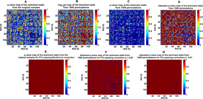
A: p-value map obtained from performing ANCOVA on each FC’s strengths in the dominant subject-specific states of the original/real three groups. B: All FCs’ associated −log₁₀ (p) map from the permutation test, where the p values (i.e., the frequencies or tail probabilities) were computed based on ANCOVA results of the dominant state from 1000 permutations. C: All FCs’ associated p-value map from the permutation test. D: Adjusted p-value map of the dominant sate for the permutation test using the step-down minP method. E: p-values of the identified 30 FCs using the original three groups after Bonferroni correction (p < 0.05). F: Adjusted p-values of the identified 58 FCs showing group difference after correction with p < 0.05 based on the adjusted p-values. G: Adjusted p-values of the identified 357 FCs showing group difference after correction with p < 0.01 based on the adjusted p-values.

4. Discussions and conclusion

Clinical high risk individuals have an increased risk of developing a psychotic disorder. Measures identified from neuroimaging data are expected to reveal the neural mechanism of CHR and schizophrenia. Recently, dynamic functional connectivity (Calhoun et al., 2014) has shown sensitivity in investigating disease biomarker for schizophrenia (Damaraju et al., 2014; Du et al., 2017; Du et al., 2016; Rashid et al., 2016; Rashid et al., 2014; Yu et al., 2015). The current study is the first to examine DFC in a CHR sample, although prior SFC-based work (Dutt et al., 2015; Smieskova et al., 2013) has observed aberrant connectivity in CHR individuals. By applying the GIG-ICA method (Du et al., 2017; Du et al., 2015) to whole-brain DFC derived from resting-state fMRI data, we investigated group differences among HC, CHR and ESZ groups.

We found that multiple FCs in the dominant state altered in CHR and ESZ groups. The primary abnormal FCs included the connections within cerebellum, between temporal cortex and cerebellum, between frontal cortex and thalamus, between supplementary motor area and parahippocampal gyrus, between supplementary motor area and temporal cortex, between postcentral and temporal cortex, between parahippocampal gyrus and temporal cortex, and between Hesch1’s gyrus and cerebellum. Our findings are in agreement with previous studies using task-related or resting-state fMRI data, which also observed abnormalities in CHR and schizophrenia groups in the frontal lobes (Allen et al., 2011; Anticevic et al., 2015; Fusar-Poli et al., 2011; Morey et al., 2005; Wang et al., 2016; Yoon et al., 2015), temporal lobes (Allen et al., 2011; Yoon et al., 2015), cerebellum (Anticevic et al., 2015; Broome et al., 2010b; Pauly et al., 2010; Wang et al., 2016), thalamus (Anticevic et al., 2015; Seiferth et al., 2008), hippocampus (Allen et al., 2011; Seiferth et al., 2008), postcentral gyrus (Broome et al., 2010a), sensory motor cortex (Anticevic et al., 2015) and Heschl’s gyrus (Anticevic et al., 2015). While cerebellum dysfunction has been suggested to be relevant to certain characteristics in some neuropsychiatric disorders (Konarski et al., 2005) including SZ (Andreasen and Pierson, 2008; Collin et al., 2011; Guo et al., 2015; Mouchet-Mages et al., 2007; Shevelkin et al., 2014; Yeganeh-Doost et al., 2011), our findings also underscore the cerebellar abnormality (Buckner, 2013; Yeganeh-Doost et al., 2011) of resting-state brain connectivity in CHR and ESZ individuals. Importantly, our previous studies using the similar dynamic connectivity analysis framework (Du et al., 2017; Du et al., 2015) also revealed significant group differences in cerebellum-related connectivity among bipolar disorder with psychosis, schizoaffective disorder and schizophrenia.

Interestingly, our results from the dominant connectivity state suggest that ESZ patients showed greater connectivity changes than CHR individuals, and in general CHR individuals had an intermediate FC pattern between HCs and ESZ patients. Measured by the mean connectivity strength, most of the identified FCs (25 of 30 FCs) in the CHR group fell in between those of the HC and ESZ groups. This may reflect large abnormalities in the subset of CHRs who are destined to transition to psychosis, with other CHRs showing normal FC patterns, or it may reflect attenuated FC abnormalities across most CHR individuals that worsen to the levels seen in ESZ patients during the transition to psychosis and its immediate aftermath. Unfortunately, the absence of sufficient clinical follow-up data in our CHR sample prevents us from distinguishing these possibilities.

Examined by two-sample t-tests, the ESZ group exhibited significant alterations compared to both HC and CHR groups in some FCs, which primarily involved the within-cerebellum connections, the connections between frontal gyri and thalamus, as well as the connections between temporal gyri and cerebellum. So, these abnormalities may not be apparent until early in the course of schizophrenia. Measured by the mean connectivity strength, the within-cerebellum connections as well as the connections between the frontal gyri and the thalamus showed a decreased trend from the HC group to the CHR group to the ESZ group, while the connections between the temporal gyri and the cerebellum increased across the three groups. Previous work (Anticevic et al., 2015) also showed hypoconnectivity in CHR individuals between thalamus and prefrontal areas, which is more prominent in those who converted to full-blown illness. Especially, five cerebellar crus related connections linking the cerebellar crus and the temporal lobe showed negative strengths in HC and CHR groups, but showed significant impairments (loss of negative connectivity) in ESZ group tested by two-sample t-tests. Habas et al (Habas et al., 2009) have shown that cerebellar crus I and II make a significant contribution to parallel cortico-cerebellar loops that are involved in executive control, salience detection, episodic memory and self-reflection. Our findings is also consistent with misconnection in a cortico-cerebellar-thalamo-cortical (CCTC) network (Andreasen, 1999), underlying the pathophysiology of schizophrenia.

Furthermore, CHR and ESZ groups shared common impairments with respect to 12 connections that were mainly associated with the supplementary motor area, parahippocampal gyrus, temporal cortex, postcentral gyrus, cerebellum, frontal gyrus, and thalamus. In these connections, 9 connections showed a deceasing trend in strength in the CHR and ESZ groups than the HC group, while 3 connections had an increasing trend in the CHR and ESZ groups compared to the HC group. Specifically, compared to the HC group, CHR and ESZ groups showed enhanced negative connectivity strengths between the right middle frontal gyrus (including orbital part) and the right thalamus, and diminished positive connectivity strengths between the left/right parahippocampal gyrus and the right temporal pole. In addition, CHR and ESZ groups also had enhanced negative functional connectivity strengths between the right supplementary motor area and left parahippocampal gyrus as well as between the right supplementary motor area and the left temporal pole (middle temporal gyrus). These abnormalities may reflect the vulnerability to develop psychosis irrespective of whether a psychotic disorder has actually developed.

Additionally, the CHR group also exhibited a group-specific abnormality in the connections between the medial part of the superior frontal gyrus and the calcarine cortex. Furthermore, FC-symptom correlations supported the clinical relevance of three connections. Two hypoconnectivities (with decreasing strength across the HC, CHR and ESZ groups) between right supplementary motor area and left parahippocampal gyrus and between right parahippocampal gyrus and right temporal pole were negatively correlated with SOPS positive symptom scores in CHR individuals. One hyperconnectivity (with increasing strength from the HC group to CHR group to ESZ group) linking right temporal pole and left cerebellum was positively correlated with PANSS negative symptom scores in ESZ patients.

Moreover, since DFC can discover multiple inherent connectivity states, our findings suggested that the non-dominant group-specific connectivity states including GS 2, GS 3, GS 4 and GS 5 showed a more similar pattern between the CHR group and ESZ group than between the HC group and CHR (or ESZ) group, indicating that these states could be disease-related.

In our study, we applied GIG-ICA to dynamic connectivity of each group separately in order to estimate the group-specific connectivity states. Our results using the permutation test support that the identified group differences in the dominant state are valid. In the supplementary materials, we also report the results obtained from performing GIG-ICA on the temporally concatenated dynamic connectivity of all subjects of the three groups to estimate the group-level and then subject-level connectivity states. Fig. S3A–B indicate that the five reliable group-level connectivity states estimated from all subjects of the three groups showed comparable patterns with the states estimated from seprate group. Furthermore, the p-values in ANCOVA of all connections (Fig. S3C) had a similar pattern to the p-values that were calculated based on the dominant SSs obtained from performing separate GIG-ICA on each group. Among the FCs with group differences (p < 0.0005) shown in Fig. S3D, 24 FCs were overlapping with the 30 FCs identified using the separate GIG-ICA one each group. The ANCOVA results of the 24 FCs are included in Table S4. For each of the 24 FCs, the inter-group differences between any pair of groups (supplementary Fig. S4) were highly consistent to that found using the separate GIG-ICA.

The present work has several limitations. (1) We lack sufficient clinical follow-up of CHR individuals to permit evaluation of whether DFC abnormalities predict conversion to psychosis. However, our framework can be potentially applied for individual-subject classification (or prediction) in future work where the clinical follow-up data of CHR subjects are available. One possible strategy is to use features from the dominant state that shows a comparable pattern across subjects. Based on the altered connectivities in the dominant connectivity state, a classifier/model can be built using converted and unconverted CHR subjects’ data. Then, for a new/testing CHR subject, the related dominant subject-specific connectivity state can be computed from the individual-subject’s dynamic connectivity patterns. Finally, the new CHR subject with features from its dominant state can be classified by the well-trained model. The other alternative strategy is to employ all states, similar to the previous work (Rashid et al., 2016) from our group. In this strategy, two groups of the group-level connectivity states (including all the dominant and non-dominant states) from both converted CHR group and unconverted CHR group can be used as the common regressors. By representing each window-related connectivity matrix as a linear combination of the common regressors and then averaging the beta-values across all windows, each subject will have same number of features. So, these features can be used to train a classifier based on the training subjects and yield the classification labels for testing subjects. We will investigate this issue in the future when more data are available. (2) The fMRI data used in our study was relatively short (i.e., six minutes). Some work (Leonardi et al., 2013) used data from a longer scanning to investigate dynamics; however, many studies have already shown that different connectivity states can be robustly and replicably captured in a similarly short period such as five minutes (Abrol et al., 2016; Calhoun et al., 2014; Damaraju et al., 2014; Miller et al., 2016; Rashid et al., 2014; Yaesoubi et al., 2015; Yu et al., 2015). (3) The number of ICs in the framework was adjustable, and a change in this parameter may influence the states and the identified biomarkers. We selected the number of ICs according to previous work (Du et al., 2017; Miller et al., 2016; Yaesoubi et al., 2015), which preserved enough variance from each subject’s DFC and resulted in reliable GSs under multiple ICA runs. However, other settings may deserve study. (4) We used the canonical AAL template-defined ROIs to compute the whole-brain FC, as the template provides clear parcellation and explicit description on whole-brain regions. In the future, we will also consider using ROIs obtained from ICA (Allen et al., 2014; Sohn et al., 2015; Yaesoubi et al., 2015), clustering techniques (Craddock et al., 2012; Du et al., 2012; Thirion et al., 2014), and previous fMRI studies (Du et al., 2016). (5) In light of the relatively small sample sizes available for this study, we included CHR individuals who were treated with antipsychotic medication at the time of testing. Given that only a minority of CHR individuals were taking antipsychotic medication, this was unlikely to confound our results. Nonetheless, we also performed the same DFC analyses using the unmedicated CHR individuals to explore. Results in supplementary materials showed that the patterns remain consistent with the findings described above. In addition, data of CHR individuals with different syndromes were analyzed. Due to the unbalanced number in different syndrome-related groups, we cannot investigate if CHR subjects with different syndromes have significant different brain connectivity. We plan to explore this issue when more data are available. (6) The association relationship (correlations) between connectivity strengths and symptom scores cannot pass correction for multiple comparisons probably due to the small sample size. So, the association results should be validated in future. (7) Similar to a previous functional connectivity study in CHR individuals (Shim et al., 2010), we regressed out the global mean signal when preprocessing, since global signal is assumed to reflect a combination of resting-state fluctuations, physiological noise (e.g. respiratory and cardiac noise), and other noise signals with non-neural origin. Regressing out global mean has been shown to facilitate the detection of localized neuronal signals and improve the specificity of functional connectivity analysis (Chai et al., 2012; Fox et al., 2005; Fox et al., 2009; Van Dijk et al., 2010), although it could result in increased negative correlations (Murphy et al., 2009). Considering that regressing out global mean is a controversial issue (Hayasaka, 2013), we will investigate its impact in the future. (8) Since the non-dominant group-level states were not very corresponding across the three groups (as shown in Fig. 2, Fig. 3 and Table 2), estimating and comparing the associated non-dominant subject-specific states should be carefully conducted. In fact, the non-dominant states may only be comparable between the CHR group and ESZ group, but not comparable between the HC group and CHR (or ESZ) group, due to that they may be disease-related. Hence, we do not include analyses on the non-dominant subject-specific states in the present study.

By applying a novel DFC method, we found widespread connectivity alterations in both CHR and ESZ groups, and ESZ patients generally showed more connectivity differences with larger changes relative to controls than CHR individuals. The functional abnormalities are generally consistent with the CCTC network postulated to underlie the core cognitive deficit of schizophrenia. Furthermore, the CHR group also showed group-specific impairments, indicating that some connections’ alterations differentiated CHR and ESZ groups. An important future research direction is to examine the extent to which the aberrant FCs identified in CHR individuals are predictive of subsequent transition to a full-blown psychotic disorder.

Table 3.

The 30 identified FCs reflecting significant group difference in analysis of covariance (ANCOVA) (p < 0.05 with Bonferroni correction) based on the dominant subject-specific connectivity states (SSs). Indexes (IDs) and names of two regions of interest (ROIs) associated with each FC, the F-value, p-value in ANCOVA of the FC are included.

ROI ID	ROI name	ROI ID	ROI name	F-value	p-value
91	Cerebellum-Crus1-L	102	Cerebellum-7b-R	20.45	1.03e–08
82	Temporal-Sup-R	103	Cerebellum-8-L	20.21	1.26e–08
82	Temporal-Sup-R	101	Cerebellum-7b-L	19.35	2.54e–08
82	Temporal-Sup-R	104	Cerebellum-8-R	17.88	8.54e–08
4	Frontal-Sup-R	77	Thalamus-L	17.22	1.48e–07
20	Supp-Motor-Area-R	39	ParaHippocampal-L	16.61	2.47e–07
79	Heschl-L	91	Cerebellum-Crus1-L	15.66	5.53e–07
88	Temporal-Pole-Mid-R	93	Cerebellum-Crus2-L	15.31	7.43e–07
88	Temporal-Pole-Mid-R	115	Vermis-9	15.07	9.08e–07
8	Frontal-Mid-R	78	Thalamus-R	14.92	1.03e–06
4	Frontal-Sup-R	78	Thalamus-R	14.70	1.25e–06
91	Cerebellum-Crus1-L	94	Cerebellum-Crus2-R	14.58	1.38e–06
82	Temporal-Sup-R	87	Temporal-Pole-Mid-L	14.30	1.75e–06
82	Temporal-Sup-R	91	Cerebellum-Crus1-L	14.07	2.15e–06
20	Supp-Motor-Area-R	87	Temporal-Pole-Mid-L	13.84	2.61e–06
86	Temporal-Mid-R	93	Cerebellum-Crus2-L	13.72	2.90e–06
79	Heschl-L	93	Cerebellum-Crus2-L	13.71	2.92e–06
81	Temporal-Sup-L	101	Cerebellum-7b-L	13.70	2.96e–06
57	Postcentral-L	87	Temporal-Pole-Mid-L	13.32	4.11e–06
17	Rolandic-Oper-L	86	Temporal-Mid-R	13.32	4.12e–06
7	Frontal-Mid-L	78	Thalamus-R	13.32	4.12e–06
39	ParaHippocampal-L	84	Temporal-Pole-Sup-R	13.25	4.37e–06
40	ParaHippocampal-R	84	Temporal-Pole-Sup-R	13.19	4.58e–06
24	Frontal-Sup-Medial-R	43	Calcarine-L	13.18	4.64e–06
69	Paracentral-Lobule-L	101	Cerebellum-7b-L	13.07	5.10e–06
82	Temporal-Sup-R	102	Cerebellum-7b-R	12.94	5.72e–06
10	Frontal-Mid-Orb-R	78	Thalamus-R	12.83	6.30e–06
57	Postcentral-L	86	Temporal-Mid-R	12.74	6.80e–06
85	Temporal-Mid-L	106	Cerebellum-9-R	12.73	6.87e–06
23	Frontal-Sup-Medial-L	43	Calcarine-L	12.65	7.38e–06

References

- Abrol A, Chaze C, Damaraju E, Calhoun VD. The Chronnectome: Replicability of Dynamic Connectivity Patterns in 7500 Resting fMRI Datasets. IEEE Engineering in Medicine and Biology Conference. 2016 doi: 10.1109/EMBC.2016.7591989. [DOI] [PubMed] [Google Scholar]
- Allen EA, Damaraju E, Plis SM, Erhardt EB, Eichele T, Calhoun VD. Tracking whole-brain connectivity dynamics in the resting state. Cereb Cortex. 2014;24:663–676. doi: 10.1093/cercor/bhs352. [DOI] [PMC free article] [PubMed] [Google Scholar]
- Allen P, Seal ML, Valli I, Fusar-Poli P, Perlini C, Day F, Wood SJ, Williams SC, McGuire PK. Altered prefrontal and hippocampal function during verbal encoding and recognition in people with prodromal symptoms of psychosis. Schizophr Bull. 2011;37:746–756. doi: 10.1093/schbul/sbp113. [DOI] [PMC free article] [PubMed] [Google Scholar]
- Amari S, Cichocki A, Yang HH. A new learning algorithm for blind signal separation. Advances in Neural Information Processing Systems. 1996;8:757–763. [Google Scholar]
- Andreasen NC. A unitary model of schizophrenia: Bleuler’s “fragmented phrene” as schizencephaly. Arch Gen Psychiatry. 1999;56:781–787. doi: 10.1001/archpsyc.56.9.781. [DOI] [PubMed] [Google Scholar]
- Andreasen NC, Pierson R. The role of the cerebellum in schizophrenia. Biol Psychiatry. 2008;64:81–88. doi: 10.1016/j.biopsych.2008.01.003. [DOI] [PMC free article] [PubMed] [Google Scholar]
- Anticevic A, Haut K, Murray JD, Repovs G, Yang GJ, Diehl C, McEwen SC, Bearden CE, Addington J, Goodyear B, Cadenhead KS, Mirzakhanian H, Cornblatt BA, Olvet D, Mathalon DH, McGlashan TH, Perkins DO, Belger A, Seidman LJ, Tsuang MT, van Erp TGM, Walker EF, Hamann S, Woods SW, Qiu ML, Cannon TD. Association of Thalamic Dysconnectivity and Conversion to Psychosis in Youth and Young Adults at Elevated Clinical Risk. JAMA Psychiatry. 2015;72:882–891. doi: 10.1001/jamapsychiatry.2015.0566. [DOI] [PMC free article] [PubMed] [Google Scholar]
- Auer DP. Spontaneous low-frequency blood oxygenation level-dependent fluctuations and functional connectivity analysis of the ‘resting’ brain. Magn Reson Imaging. 2008;26:1055–1064. doi: 10.1016/j.mri.2008.05.008. [DOI] [PubMed] [Google Scholar]
- Bassett DS, Bullmore ET. Human brain networks in health and disease. Curr Opin Neurol. 2009;22:340–347. doi: 10.1097/WCO.0b013e32832d93dd. [DOI] [PMC free article] [PubMed] [Google Scholar]
- Bell AJ, Sejnowski TJ. An information-maximization approach to blind separation and blind deconvolution. Neural Comput. 1995;7:1129–1159. doi: 10.1162/neco.1995.7.6.1129. [DOI] [PubMed] [Google Scholar]
- Borgwardt S, Koutsouleris N, Aston J, Studerus E, Smieskova R, Riecher-Rossler A, Meisenzahl EM. Distinguishing prodromal from first-episode psychosis using neuroanatomical single-subject pattern recognition. Schizophr Bull. 2013;39:1105–1114. doi: 10.1093/schbul/sbs095. [DOI] [PMC free article] [PubMed] [Google Scholar]
- Broome MR, Fusar-Poli P, Matthiasson P, Woolley JB, Valmaggia L, Johns LC, Tabraham P, Bramon E, Williams SCR, Brammer MJ, Chitnis X, Zelaya F, McGuire PK. Neural correlates of visuospatial working memory in the ‘at-risk mental state’. Psychol Med. 2010a;40:1987–1999. doi: 10.1017/S0033291710000280. [DOI] [PubMed] [Google Scholar]
- Broome MR, Matthiasson P, Fusar-Poli P, Woolley JB, Johns LC, Tabraham P, Bramon E, Valmaggia L, Williams SC, Brammer MJ, Chitnis X, McGuire PK. Neural correlates of movement generation in the ‘at-risk mental state’. Acta Psychiatr Scand. 2010b;122:295–301. doi: 10.1111/j.1600-0447.2009.01524.x. [DOI] [PubMed] [Google Scholar]
- Buckner RL. The cerebellum and cognitive function: 25 years of insight from anatomy and neuroimaging. Neuron. 2013;80:807–815. doi: 10.1016/j.neuron.2013.10.044. [DOI] [PubMed] [Google Scholar]
- Calhoun VD, Adali T. Multisubject independent component analysis of fMRI: a decade of intrinsic networks, default mode, and neurodiagnostic discovery. IEEE Rev Biomed Eng. 2012;5:60–73. doi: 10.1109/RBME.2012.2211076. [DOI] [PMC free article] [PubMed] [Google Scholar]
- Calhoun VD, Miller R, Pearlson GD, Adali T. The Chronnectome: Time-Varying Connectivity Networks as the Next Frontier in fMRI Data Discovery. Neuro. 2014;84:262–274. doi: 10.1016/j.neuron.2014.10.015. [DOI] [PMC free article] [PubMed] [Google Scholar]
- Cannon TD, Cadenhead K, Cornblatt B, Woods SW, Addington J, Walker E, Seidman LJ, Perkins D, Tsuang M, McGlashan T, Heinssen R. Prediction of psychosis in youth at high clinical risk. Archives of General Psychiatry. 2008;65:28–37. doi: 10.1001/archgenpsychiatry.2007.3. [DOI] [PMC free article] [PubMed] [Google Scholar]
- Chai XQJ, Castanon AN, Ongur D, Whitfield-Gabrieli S. Anticorrelations in resting state networks without global signal regression. Neuroimage. 2012;59:1420–1428. doi: 10.1016/j.neuroimage.2011.08.048. [DOI] [PMC free article] [PubMed] [Google Scholar]
- Collin G, Hulshoff Pol HE, Haijma SV, Cahn W, Kahn RS, van den Heuvel MP. Impaired cerebellar functional connectivity in schizophrenia patients and their healthy siblings. Front Psychiatry. 2011;2:73. doi: 10.3389/fpsyt.2011.00073. [DOI] [PMC free article] [PubMed] [Google Scholar]
- Cordes D, Haughton VM, Arfanakis K, Carew JD, Turski PA, Moritz CH, Quigley MA, Meyerand ME. Frequencies contributing to functional connectivity in the cerebral cortex in “resting-state” data. AJNR Am J Neuroradiol. 2001;22:1326–1333. [PMC free article] [PubMed] [Google Scholar]
- Craddock RC, James GA, Holtzheimer PE, 3rd, Hu XP, Mayberg HS. A whole brain fMRI atlas generated via spatially constrained spectral clustering. Hum Brain Mapp. 2012;33:1914–1928. doi: 10.1002/hbm.21333. [DOI] [PMC free article] [PubMed] [Google Scholar]
- Damaraju E, Allen EA, Belger A, Ford JM, McEwen S, Mathalon DH, Mueller BA, Pearlson GD, Potkin SG, Preda A, Turner JA, Vaidya JG, van Erp TG, Calhoun VD. Dynamic functional connectivity analysis reveals transient states of dysconnectivity in schizophrenia. Neuroimage Clin. 2014;5:298–308. doi: 10.1016/j.nicl.2014.07.003. [DOI] [PMC free article] [PubMed] [Google Scholar]
- Di X, Biswal BB. Dynamic brain functional connectivity modulated by resting-state networks. Brain Struct Funct. 2015;220:37–46. doi: 10.1007/s00429-013-0634-3. [DOI] [PMC free article] [PubMed] [Google Scholar]
- Du YH, Fan Y. Group information guided ICA for fMRI data analysis. Neuroimage. 2013;69:157–197. doi: 10.1016/j.neuroimage.2012.11.008. [DOI] [PubMed] [Google Scholar]
- Du YH, Li HM, Wu H, Fan Y. Identification of subject specific and functional consistent ROIs using semi-supervised learning. Proceedings of SPIE, Medical Imaging. 2012;2012 Image Processing 8314. [Google Scholar]
- Du YH, Pearlson G, Lin DD, Sui J, Chen JY, Salman M, Tamminga C, Ivleva EI, Sweeney J, Keshavan M, Clementz B, Bustillo J, Calhoun V. Identifying dynamic functional connectivity biomarkers using GIG-ICA: application to schizophrenia, schizoaffective disorder and psychotic bipolar disorder. Hum Brain Mapp. 2017;38:2683–2708. doi: 10.1002/hbm.23553. [DOI] [PMC free article] [PubMed] [Google Scholar]
- Du YH, Pearlson GD, He H, Wu L, Y CJ, Calhoun VD. Identifying brain dynamic network states via GIG-ICA: Application to schizophrenia, bipolar and schizoaffective disorders. IEEE 12th International Symposium on Biomedical Imaging (ISBI) 2015:478–481. [Google Scholar]
- Du YH, Pearlson GD, Yu Q, He H, Lin DD, Sui J, Wu L, Calhoun VD. Interaction among subsystems within default mode network diminished in schizophrenia patients: A dynamic connectivity approach. Schizophr Res. 2016;170:55–65. doi: 10.1016/j.schres.2015.11.021. [DOI] [PMC free article] [PubMed] [Google Scholar]
- Dutt A, Tseng HH, Fonville L, Drakesmith M, Su L, Evans J, Zammit S, Jones D, Lewis G, David AS. Exploring neural dysfunction in ‘clinical high risk’ for psychosis: a quantitative review of fMRI studies. J Psychiatr Res. 2015;61:122–134. doi: 10.1016/j.jpsychires.2014.08.018. [DOI] [PubMed] [Google Scholar]
- Erhardt EB, Rachakonda S, Bedrick EJ, Allen EA, Adali T, Calhoun VD. Comparison of multi-subject ICA methods for analysis of fMRI data. Hum Brain Mapp. 2011;32:2075–2095. doi: 10.1002/hbm.21170. [DOI] [PMC free article] [PubMed] [Google Scholar]
- Fox MD, Snyder AZ, Vincent JL, Corbetta M, Van Essen DC, Raichle ME. The human brain is intrinsically organized into dynamic, anticorrelated functional networks. Proceedings of the National Academy of Sciences of the United States of America. 2005;102:9673–9678. doi: 10.1073/pnas.0504136102. [DOI] [PMC free article] [PubMed] [Google Scholar]
- Fox MD, Zhang D, Snyder AZ, Raichle ME. The global signal and observed anticorrelated resting state brain networks. J Neurophysiol. 2009;101:3270–3283. doi: 10.1152/jn.90777.2008. [DOI] [PMC free article] [PubMed] [Google Scholar]
- Friedman J, Hastie T, Tibshirani R. Sparse inverse covariance estimation with the graphical lasso. Biostatistics. 2008;9:432–441. doi: 10.1093/biostatistics/kxm045. [DOI] [PMC free article] [PubMed] [Google Scholar]
- Fryer SL, Woods SW, Kiehl KA, Calhoun VD, Pearlson GD, Roach BJ, Ford JM, Srihari VH, McGlashan TH, Mathalon DH. Deficient Suppression of Default Mode Regions during Working Memory in Individuals with Early Psychosis and at Clinical High-Risk for Psychosis. Front Psychiatry. 2013;4:92. doi: 10.3389/fpsyt.2013.00092. [DOI] [PMC free article] [PubMed] [Google Scholar]
- Fusar-Poli P, Bonoldi I, Yung AR, Borgwardt S, Kempton MJ, Valmaggia L, Barale F, Caverzasi E, McGuire P. Predicting psychosis: meta-analysis of transition outcomes in individuals at high clinical risk. Arch Gen Psychiatry. 2012;69:220–229. doi: 10.1001/archgenpsychiatry.2011.1472. [DOI] [PubMed] [Google Scholar]
- Fusar-Poli P, Howes OD, Allen P, Broome M, Valli I, Asselin MC, Montgomery AJ, Grasby PM, McGuire P. Abnormal prefrontal activation directly related to pre-synaptic striatal dopamine dysfunction in people at clinical high risk for psychosis. Mol Psychiatry. 2011;16:67–75. doi: 10.1038/mp.2009.108. [DOI] [PubMed] [Google Scholar]
- Guo WB, Liu F, Chen JD, Wu RR, Zhang ZK, Yu MY, Xiao CQ, Zhao JP. Resting-state cerebellar-cerebral networks are differently affected in first-episode, drug-naive schizophrenia patients and unaffected siblings. Scientific Reports. 2015;5 doi: 10.1038/srep17275. [DOI] [PMC free article] [PubMed] [Google Scholar]
- Habas C, Kamdar N, Nguyen D, Prater K, Beckmann CF, Menon V, Greicius MD. Distinct cerebellar contributions to intrinsic connectivity networks. Journal of Neuroscience. 2009;29:8586–8594. doi: 10.1523/JNEUROSCI.1868-09.2009. [DOI] [PMC free article] [PubMed] [Google Scholar]
- Hayasaka S. Functional connectivity networks with and without global signal correction. Front Hum Neurosci. 2013;7 doi: 10.3389/fnhum.2013.00880. [DOI] [PMC free article] [PubMed] [Google Scholar]
- Hutchison RM, Womelsdorf T, Gati JS, Everling S, Menon RS. Resting-state networks show dynamic functional connectivity in awake humans and anesthetized macaques. Hum Brain Mapp. 2013;34:2154–2177. doi: 10.1002/hbm.22058. [DOI] [PMC free article] [PubMed] [Google Scholar]
- Jung WH, Jang JH, Byun MS, An SK, Kwon JS. Structural brain alterations in individuals at ultra-high risk for psychosis: a review of magnetic resonance imaging studies and future directions. J Korean Med Sci. 2010;25:1700–1709. doi: 10.3346/jkms.2010.25.12.1700. [DOI] [PMC free article] [PubMed] [Google Scholar]
- Jung WH, Jang JH, Shin NY, Kim SN, Choi CH, An SK, Kwon JS. Regional brain atrophy and functional disconnection in Broca’s area in individuals at ultra-high risk for psychosis and schizophrenia. PLoS One. 2012;7:e51975. doi: 10.1371/journal.pone.0051975. [DOI] [PMC free article] [PubMed] [Google Scholar]
- Kay SR, Fiszbein A, Opler LA. The positive and negative syndrome scale (PANSS) for schizophrenia. Schizophr Bull. 1987;13:261–276. doi: 10.1093/schbul/13.2.261. [DOI] [PubMed] [Google Scholar]
- Klosterkotter J, Hellmich M, Steinmeyer EM, Schultze-Lutter F. Diagnosing schizophrenia in the initial prodromal phase. Arch Gen Psychiatry. 2001;58:158–164. doi: 10.1001/archpsyc.58.2.158. [DOI] [PubMed] [Google Scholar]
- Konarski JZ, McIntyre RS, Grupp LA, Kennedy SH. Is the cerebellum relevant in the circuitry of neuropsychiatric disorders? Journal of Psychiatry & Neuroscience. 2005;30:178–186. [PMC free article] [PubMed] [Google Scholar]
- Leonardi N, Richiardi J, Gschwind M, Simioni S, Annoni JM, Schluep M, Vuilleumier P, Van De Ville D. Principal components of functional connectivity: a new approach to study dynamic brain connectivity during rest. Neuroimage. 2013;83:937–950. doi: 10.1016/j.neuroimage.2013.07.019. [DOI] [PubMed] [Google Scholar]
- Li X, Zhu D, Jiang X, Jin C, Zhang X, Guo L, Zhang J, Hu X, Li L, Liu T. Dynamic functional connectomics signatures for characterization and differentiation of PTSD patients. Hum Brain Mapp. 2014;35:1761–1778. doi: 10.1002/hbm.22290. [DOI] [PMC free article] [PubMed] [Google Scholar]
- Ma S, Correa NM, Li XL, Eichele T, Calhoun VD, Adali T. Automatic identification of functional clusters in FMRI data using spatial dependence. IEEE Trans Biomed Eng. 2011;58:3406–3417. doi: 10.1109/TBME.2011.2167149. [DOI] [PMC free article] [PubMed] [Google Scholar]
- McGlashan T, Walsh BC, Woods SW. The Psychosis-Risk Syndrome 2010 [Google Scholar]
- Miller RL, Yaesoubi M, Turner JA, Mathalon D, Preda A, Pearlson G, Adali T, Calhoun VD. Higher Dimensional Meta-State Analysis Reveals Reduced Resting fMRI Connectivity Dynamism in Schizophrenia Patients. PLoS One. 2016;11:e0149849. doi: 10.1371/journal.pone.0149849. [DOI] [PMC free article] [PubMed] [Google Scholar]
- Miller TJ, McGlashan TH, Rosen JL, Cadenhead K, Cannon T, Ventura J, McFarlane W, Perkins DO, Pearlson GD, Woods SW. Prodromal assessment with the structured interview for prodromal syndromes and the scale of prodromal symptoms: predictive validity, interrater reliability, and training to reliability. Schizophr Bull. 2003;29:703–715. doi: 10.1093/oxfordjournals.schbul.a007040. [DOI] [PubMed] [Google Scholar]
- Morey RA, Inan S, Mitchell TV, Perkins DO, Lieberman JA, Belger A. Imaging frontostriatal function in ultra-high-risk, early, and chronic schizophrenia during executive processing. Arch Gen Psychiatry. 2005;62:254–262. doi: 10.1001/archpsyc.62.3.254. [DOI] [PMC free article] [PubMed] [Google Scholar]
- Mouchet-Mages S, Canceil O, Willard D, Krebs MO, Cachia A, Martinot JL, Rodrigo S, Oppenheim C, Meder JF. Sensory dysfunction is correlated to cerebellar volume reduction in early schizophrenia. Schizophr Res. 2007;91:266–269. doi: 10.1016/j.schres.2006.11.031. [DOI] [PubMed] [Google Scholar]
- Murphy K, Birn RM, Handwerker DA, Jones TB, Bandettini PA. The impact of global signal regression on resting state correlations: are anti-correlated networks introduced? Neuroimage. 2009;44:893–905. doi: 10.1016/j.neuroimage.2008.09.036. [DOI] [PMC free article] [PubMed] [Google Scholar]
- Pauly K, Seiferth NY, Kellermann T, Ruhrmann S, Daumann B, Backes V, Klosterkotter J, Shah NJ, Schneider F, Kircher TT, Habel U. The interaction of working memory and emotion in persons clinically at risk for psychosis: An fMRI pilot study. Schizophr Res. 2010;120:167–176. doi: 10.1016/j.schres.2009.12.008. [DOI] [PubMed] [Google Scholar]
- Rashid B, Arbabshirani MR, Damaraju E, Cetin MS, Miller R, Pearlson GD, Calhoun VD. Classification of schizophrenia and bipolar patients using static and dynamic resting-state fMRI brain connectivity. Neuroimage. 2016;134:645–657. doi: 10.1016/j.neuroimage.2016.04.051. [DOI] [PMC free article] [PubMed] [Google Scholar]
- Rashid B, Damaraju E, Pearlson GD, Calhoun VD. Dynamic connectivity states estimated from resting fMRI Identify differences among Schizophrenia, bipolar disorder, and healthy control subjects. Front Hum Neurosci. 2014;8 doi: 10.3389/fnhum.2014.00897. [DOI] [PMC free article] [PubMed] [Google Scholar]
- Schmidt A, Smieskova R, Aston J, Simon A, Allen P, Fusar-Poli P, McGuire PK, Riecher-Rossler A, Stephan KE, Borgwardt S. Brain Connectivity Abnormalities Predating the Onset of Psychosis Correlation With the Effect of Medication. JAMA Psychiatry. 2013;70:903–912. doi: 10.1001/jamapsychiatry.2013.117. [DOI] [PubMed] [Google Scholar]
- Seiferth NY, Pauly K, Habel U, Kellermann T, Shah NJ, Ruhrmann S, Klosterkotter J, Schneider F, Kircher T. Increased neural response related to neutral faces in individuals at risk for psychosis. Neuroimage. 2008;40:289–297. doi: 10.1016/j.neuroimage.2007.11.020. [DOI] [PubMed] [Google Scholar]
- Shevelkin AV, Ihenatu C, Pletnikov MV. Pre-clinical models of neurodevelopmental disorders: focus on the cerebellum. Rev Neurosci. 2014;25:177–194. doi: 10.1515/revneuro-2013-0049. [DOI] [PMC free article] [PubMed] [Google Scholar]
- Shim G, Oh JS, Jung WH, Jang JH, Choi CH, Kim E, Park HY, Choi JS, Jung MH, Kwon JS. Altered resting-state connectivity in subjects at ultra-high risk for psychosis: an fMRI study. Behavioral and Brain Functions. 2010;6 doi: 10.1186/1744-9081-6-58. [DOI] [PMC free article] [PubMed] [Google Scholar]
- Smieskova R, Marmy J, Schmidt A, Bendfeldt K, Riecher-Rossler A, Walter M, Lang UE, Borgwardt S. Do Subjects at Clinical High Risk for Psychosis Differ from those with a Genetic High Risk? - A Systematic Review of Structural and Functional Brain Abnormalities. Current Medicinal Chemistry. 2013;20:467–481. doi: 10.2174/0929867311320030018. [DOI] [PMC free article] [PubMed] [Google Scholar]
- Smith SM, Miller KL, Salimi-Khorshidi G, Webster M, Beckmann CF, Nichols TE, Ramsey JD, Woolrich MW. Network modelling methods for FMRI. Neuroimage. 2011;54:875–891. doi: 10.1016/j.neuroimage.2010.08.063. [DOI] [PubMed] [Google Scholar]
- Sohn WS, Yoo K, Lee YB, Seo SW, Na DL, Jeong Y. Influence of ROI selection on resting state functional connectivity: an individualized approach for resting state fMRI analysis. Front Neurosci. 2015;9:280. doi: 10.3389/fnins.2015.00280. [DOI] [PMC free article] [PubMed] [Google Scholar]
- Sporns O. Contributions and challenges for network models in cognitive neuroscience. Nat Neurosci. 2014;17:652–660. doi: 10.1038/nn.3690. [DOI] [PubMed] [Google Scholar]
- Thirion B, Varoquaux G, Dohmatob E, Poline JB. Which fMRI clustering gives good brain parcellations? Front Neurosci. 2014;8 doi: 10.3389/fnins.2014.00167. [DOI] [PMC free article] [PubMed] [Google Scholar]
- Tzourio-Mazoyer N, Landeau B, Papathanassiou D, Crivello F, Etard O, Delcroix N, Mazoyer B, Joliot M. Automated anatomical labeling of activations in SPM using a macroscopic anatomical parcellation of the MNI MRI single-subject brain. Neuroimage. 2002;15:273–289. doi: 10.1006/nimg.2001.0978. [DOI] [PubMed] [Google Scholar]
- van den Heuvel MP, Hulshoff Pol HE. Exploring the brain network: a review on resting-state fMRI functional connectivity. Eur Neuropsychopharmacol. 2010;20:519–534. doi: 10.1016/j.euroneuro.2010.03.008. [DOI] [PubMed] [Google Scholar]
- Van Dijk KRA, Hedden T, Venkataraman A, Evans KC, Lazar SW, Buckner RL. Intrinsic Functional Connectivity As a Tool For Human Connectomics: Theory, Properties, and Optimization. J Neurophysiol. 2010;103:297–321. doi: 10.1152/jn.00783.2009. [DOI] [PMC free article] [PubMed] [Google Scholar]
- Ventura J, Liberman RP, Green MF, Shaner A, Mintz J. Training and quality assurance with the Structured Clinical Interview for DSM-IV (SCID-I/P) Psychiatry Res. 1998;79:163–173. doi: 10.1016/s0165-1781(98)00038-9. [DOI] [PubMed] [Google Scholar]
- Wang HL, Guo WB, Liu F, Wang GD, Lyu HL, Wu RR, Chen JD, Wang S, Li LH, Zhao JP. Patients with first-episode, drug-naive schizophrenia and subjects at ultra-high risk of psychosis shared increased cerebellar-default mode network connectivity at rest. Scientific Reports. 2016;6 doi: 10.1038/srep26124. [DOI] [PMC free article] [PubMed] [Google Scholar]
- Xia M, Wang J, He Y. BrainNet Viewer: a network visualization tool for human brain connectomics. PLoS One. 2013;8:e68910. doi: 10.1371/journal.pone.0068910. [DOI] [PMC free article] [PubMed] [Google Scholar]
- Yaesoubi M, Miller RL, Calhoun VD. Mutually temporally independent connectivity patterns: A new framework to study the dynamics of brain connectivity at rest with application to explain group difference based on gender. Neuroimage. 2015;107:85–94. doi: 10.1016/j.neuroimage.2014.11.054. [DOI] [PMC free article] [PubMed] [Google Scholar]
- Yan CG, Zang YF. DPARSF: A MATLAB Toolbox for “Pipeline” Data Analysis of Resting-State fMRI. Front Syst Neurosci. 2010;4:13. doi: 10.3389/fnsys.2010.00013. [DOI] [PMC free article] [PubMed] [Google Scholar]
- Yeganeh-Doost P, Gruber O, Falkai P, Schmitt A. The role of the cerebellum in schizophrenia: from cognition to molecular pathways. Clinics (Sao Paulo) 2011;66(Suppl 1):71–77. doi: 10.1590/S1807-59322011001300009. [DOI] [PMC free article] [PubMed] [Google Scholar]
- Yoon YB, Yun JY, Jung WH, Cho KIK, Kim SN, Lee TY, Park HY, Kwon JS. Altered Fronto-Temporal Functional Connectivity in Individuals at Ultra-High-Risk of Developing Psychosis. PLoS One. 2015;10 doi: 10.1371/journal.pone.0135347. [DOI] [PMC free article] [PubMed] [Google Scholar]
- Yu Q, Erhardt EB, Sui J, Du Y, He H, Hjelm D, Cetin MS, Rachakonda S, Miller RL, Pearlson G, Calhoun VD. Assessing dynamic brain graphs of time-varying connectivity in fMRI data: Application to healthy controls and patients with schizophrenia. Neuroimage. 2015;107:345–355. doi: 10.1016/j.neuroimage.2014.12.020. [DOI] [PMC free article] [PubMed] [Google Scholar]
- Yung AR, Phillips LJ, Yuen HP, Francey SM, McFarlane CA, Hallgren M, McGorry PD. Psychosis prediction: 12-month follow up of a high-risk (“prodromal”) group. Schizophr Res. 2003;60:21–32. doi: 10.1016/s0920-9964(02)00167-6. [DOI] [PubMed] [Google Scholar]
- Yung AR, Yuen HP, McGorry PD, Phillips LJ, Kelly D, Dell’Olio M, Francey SM, Cosgrave EM, Killackey E, Stanford C, Godfrey K, Buckby J. Mapping the onset of psychosis: the Comprehensive Assessment of At-Risk Mental States. Aust N Z J Psychiatry. 2005;39:964–971. doi: 10.1080/j.1440-1614.2005.01714.x. [DOI] [PubMed] [Google Scholar]
- Zalesky A, Breakspear M. Towards a statistical test for functional connectivity dynamics. Neuroimage. 2015;114:466–470. doi: 10.1016/j.neuroimage.2015.03.047. [DOI] [PubMed] [Google Scholar]
- Zhang D, Raichle ME. Disease and the brain’s dark energy. Nat Rev Neurol. 2010;6:15–28. doi: 10.1038/nrneurol.2009.198. [DOI] [PubMed] [Google Scholar]
- Zuo XN, Di Martino A, Kelly C, Shehzad ZE, Gee DG, Klein DF, Castellanos FX, Biswal BB, Milham MP. The oscillating brain: complex and reliable. Neuroimage. 2010;49:1432–1445. doi: 10.1016/j.neuroimage.2009.09.037. [DOI] [PMC free article] [PubMed] [Google Scholar]
Associated Data
This section collects any data citations, data availability statements, or supplementary materials included in this article.