Modified dixon‐based renal dynamic contrast‐enhanced MRI facilitates automated registration and perfusion analysis

Abstract

Purpose

Renal dynamic contrast‐enhanced (DCE) MRI provides information on renal perfusion and filtration. However, clinical implementation is hampered by challenges in postprocessing as a result of misalignment of the kidneys due to respiration. We propose to perform automated image registration using the fat‐only images derived from a modified Dixon reconstruction of a dual‐echo acquisition because these provide consistent contrast over the dynamic series.

Methods

DCE data of 10 hypertensive patients was used. Dual‐echo images were acquired at 1.5 T with temporal resolution of 3.9 s during contrast agent injection. Dixon fat, water, and in‐phase and opposed‐phase (OP) images were reconstructed. Postprocessing was automated. Registration was performed both to fat images and OP images for comparison. Perfusion and filtration values were extracted from a two‐compartment model fit.

Results

Automatic registration to fat images performed better than automatic registration to OP images with visible contrast enhancement. Median vertical misalignment of the kidneys was 14 mm prior to registration, compared to 3 mm and 5 mm with registration to fat images and OP images, respectively (P = 0.03). Mean perfusion values and MR‐based glomerular filtration rates (GFR) were 233 ± 64 mL/100 mL/min and 60 ± 36 mL/minute, respectively, based on fat‐registered images. MR‐based GFR correlated with creatinine‐based GFR (P = 0.04) for fat‐registered images. For unregistered and OP‐registered images, this correlation was not significant.

Conclusion

Absence of contrast changes on Dixon fat images improves registration in renal DCE MRI and enables automated postprocessing, resulting in a more accurate estimation of GFR. Magn Reson Med 80:66–76, 2018. © 2017 The Authors Magnetic Resonance in Medicine published by Wiley Periodicals, Inc. on behalf of International Society for Magnetic Resonance in Medicine. This is an open access article under the terms of the Creative Commons Attribution NonCommercial License, which permits use, distribution and reproduction in any medium, provided the original work is properly cited and is not used for commercial purposes.

INTRODUCTION

Dynamic contrast‐enhanced (DCE) MRI of the kidneys provides information on renal perfusion 1 and (single kidney) glomerular filtration rate ((sk)GFR) 2, 3, 4. It can be used for characterization of renal masses 5, 6, 7 and is a promising noninvasive tool for early detection of renal transplant rejection 8, 9, although the risk of nephrogenic systemic fibrosis might limit the use of contrast‐based MR techniques in this population. DCE MRI consists of acquisition of a dynamic series of images during injection of a contrast agent (CA). By fitting a pharmacokinetic model to the data, quantitative information on renal perfusion and filtration can be obtained. Although renal DCE MRI is a growing field of research, implementation in clinical practice is limited due to challenges in the postprocessing of data and a lack of standardized protocols. A main postprocessing challenge is misalignment of the kidneys in the dynamic series due to respiration. This leads to disturbances in the time‐intensity curves, which affects the pharmacokinetic model fit and therefore leads to errors in the estimation of perfusion and filtration values 10.

Numerous methods exist to deal with respiratory motion in the kidneys, with breath holding presumably the simplest and most intuitive 11. Yet, a single breath hold limits the length of the time series and requires cooperation of the patient, which is hardly achievable in diseased or pediatric populations. Alternatively, artifacts induced by respiratory motion can be minimized by respiratory gating 12, 13, but the resultant time intervals are not regular and temporal resolution is reduced. Therefore, a free‐breathing approach with retrospective motion correction often is preferred. Approaches include retrospective respiratory gating 5, 14, that is, discarding images acquired during inspiration, and image registration. Retrospective triggering again limits temporal resolution because images acquired during inspiration are removed from the dataset. Furthermore, image registration in DCE MRI is complicated by the large dynamic range in image contrast over the dynamic series. To avoid this problem, advanced registration techniques are used, such as those based on edge detection 8, 10, 15, 16, 17, 18 or mutual information 19, 20. Registration has been shown to improve estimation of filtration 21, 22.

We propose to circumvent the problem of changes in contrast enhancement through use of a Dixon reconstruction of dual‐echo DCE data, which allows for reconstruction of fat‐only images on which renal contours are intrinsically outlined. Because gadolinium‐based CAs are confined to the intravascular and extracellular compartments 23, kidney outlines are not subject to changes typically seen over the course of the DCE acquisition using conventional sequences.

Furthermore, we aim to enable automated registration and perfusion analysis of renal DCE data by implementing a combination of image registration to Dixon fat images and automated kidney delineation using the approach proposed by Zöllner et al. 19.

METHODS

Subjects

A representative selection of 10 patients (4 male, mean age 57 years, mean systolic/diastolic blood pressure 156/94 mm Hg, mean estimated glomerular filtration rate (eGFR) 80 mL/min/1.73 m²) was made out of a cohort of hypertensive patients referred for treatment with renal denervation. A detailed description of this population was published earlier 24. eGFR was estimated using the chronic kidney disease epidemiology collaboration (CKD‐EPI) equation 25 based on creatinine clearance. Plasma creatinine levels were measured within a week of the MRI. All patients underwent DCE MRI as part of the renal denervation workup. Permission from the local medical ethics review committee was obtained, and all patients signed informed consent prior to inclusion into the study.

Imaging Protocol

Dual‐echo images were acquired on a 1.5 T (Ingenia 4.1, Philips Healthcare, Eindhoven, the Netherlands) MR system using a 3D gradient‐echo dual‐echo protocol with a modified Dixon reconstruction 26. All images were acquired with repetition time of 5.9 ms and echo times of 1.8 and 4.0 ms. First, three precontrast acquisitions (prescans) with a variable flip angle (5°, 13°, and 20°) were acquired for determination of precontrast longitudinal relaxation rate (R₁). Subsequently, a dynamic series consisting of 25 dynamics with flip angle 15° was acquired. Twenty‐five coronal slices were acquired with voxel size 2.5 × 2.5 × 3.0 mm and field of view of 420 × 420 mm. Based on the work of Michaely et al. 12, we kept temporal resolution to less than 4 s per dynamic phase. Using a sensitivity‐encoding technique factor of 2.5 in left–right direction, an acquisition time of 3.9 s per dynamic was achieved. During the dynamic series, 0.1 mmol/kg of Gadovist was infused at a rate of 1 mL/s, followed by a saline flush of 25 mL. Subsequently, Dixon water‐only, fat‐only, in‐phase (IP), and opposed‐phase (OP) images were generated.

Segmentation

Postprocessing was performed with a MatLab (MatLab 2014b, MathWorks, Natick, Massachusetts, USA) graphic user interface that was developed in‐house. Kidney delineation was performed according to the image segmentation method described by Zöllner et al. 19. This approach consists of k‐means clustering of the voxel‐based time‐intensity curves obtained from the whole range of dynamics. Due to the difference between cortical and medullary time‐intensity curves, cortex and medulla usually are assigned to different clusters. To obtain parenchymal regions of interest (ROIs), cortical and medullary ROIs were combined. To improve speed and robustness of this method, we made some slight adjustments. First, because fat images were available, voxels containing mostly fatty tissue could easily be excluded using a simple thresholding approach. In adipose subjects with enough fat surrounding the kidneys, thresholding alone was sufficient to create renal masks. In the remaining subjects, thresholding diminished the computation time because adipose tissue could be excluded for clustering. The default fat threshold could be adjusted manually using a slider. Second, because the renal cluster often also encompassed the renal artery, masks were eroded and dilated to exclude the artery.

Due to smoother time‐intensity curves after registration, the segmentation algorithm performed better on registered data. Therefore, it was performed both before and after image registration. The initial rough masks (Fig. 1a) were employed to make wide crops around both kidneys to enable separate registration. The second and more precise masks (Fig. 1b) were used for calculation of whole kidney time‐intensity curves. For each segmentation, manual interaction was required to adjust the fat threshold (optionally); set the number of clusters; and label the resultant masks as kidney, cortex, or medulla.

Figure 1.

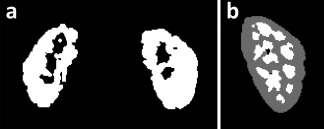
Segmentation of the kidney. (a) Rough mask created before registration, used only to crop with a wide margin around the kidney. (b) Precise cortical (gray) and medullary (white) mask created after registration. Combined, these masks form a parenchymal mask.

Segmentation of a ROI inside the aorta for determination of the arterial input function was fully automated (Fig. 2). Analogous to a maximum‐intensity projection, which consists of the maximum intensities reached in a spatial direction, a time maximum‐intensity projection was created, which consists of the maximum intensities reached in the dynamic series. On this time maximum‐intensity projection, 98% of voxels with lowest signal intensity were discarded. For the remaining voxels, components consisting of connected voxels were identified. The largest component represented the aorta. To minimize the impact of inflow often present in the cranial part of the aorta, a 5 × 8 voxel arterial ROI was placed in the most caudal row of the largest component, with a width of five voxels or more, and in seven rows above that row. No manual interaction was required.

Figure 2.

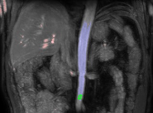
Time maximum‐intensity projection of unregistered images used for automated segmentation of aorta ROI. The 2% voxels with highest signal intensity are highlighted red and blue. The blue voxels denote the largest connected component, that is, the aorta. As caudal as possible in this component, a 5 × 8 voxel ROI is delineated in green. Although not clearly visible in this time maximum‐intensity projection, an inflow artefact also is present in the cranial parts of the aorta in this subject. ROI, region of interest.

Registration

Rigid registration was performed in 3D to the fat‐only first dynamic image using the visualisation toolkit (VTK) Registration Toolkit (v2.0.0 27, freely available at http://www.vtk.org/ (Kitware Inc, New York, New York, USA)). To enable separate registration for left and right kidneys, the initial rough renal masks were employed to create wide crops around both kidneys. Because there is no contrast enhancement in the fat images used for registration, the choice of the reference image is not pivotal. Prescans were also registered to the first dynamic. The registration procedure is illustrated in Figure 3. In our proposed method, registration is performed on fat images, which are not expected to show contrast enhancement. The obtained transformation matrices are subsequently applied to the corresponding water images, which have identical time stamps. To compare our method with the conventional approach, we also performed registration on OP images, which do show contrast enhancement. Of the available images, OP images have the lowest echo time and are probably most similar to images acquired in a standard postcontrast dynamic series. It would have been more appropriate to perform this comparison with source first echo images, but unfortunately only the reconstructed Dixon images were saved and the source images were not available.

Figure 3.

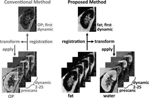
Image registration algorithm. Left: Conventional method. OP images were used because they have the shortest echo time of the images available. Registration of the prescans and dynamic 2 through 25 was performed to the first dynamic, and transformation matrices were applied to the OP images. Right: Proposed method. Registration of the prescans and dynamic 2 through 25 to the first dynamic was performed on fat images, in which no contrast enhancement is visible. Subsequently, fat transformation matrices were applied to water images. OP, opposed phase; transform, transformation matrix.

Both for registration to fat and to OP images, gradient cross‐correlation (GCC) was used as a similarity measure, but in OP images normalized mutual information (NMI) was also used to compare performance. Mutual information in image registration is discussed in detail elsewhere 28. In short, NMI does not depend on the actual intensity of the images and therefore might yield better results in registration to contrast‐enhanced OP images. Both GCC and NMI are available in the VTK registration toolbox (v2.0.0).

For the arterial ROI in the aorta, the prescans were registered to the first dynamic because replanning sometimes occurred between the prescans and the dynamics.

To quantify the resulting registration error, two metrics were used. First, as a measure of respiratory‐induced motion, root‐mean‐square (RMS) vertical misalignment of the top of the kidney was measured manually with respect to the first dynamic on all dynamics. This was repeated after registration both to OP and fat images to measure residual vertical misalignment and to allow for comparison. However, this only measured registration performance in one direction. As a second measure of registration error, the whole parenchyma time‐intensity curve was calculated on all dynamics using fat images. Assuming perfect registration, the time‐intensity curve of the whole kidney will be constant. However, because the kidneys are surrounded by adipose tissue, registration errors result in fluctuations in the whole kidney time‐intensity curve when adipose tissue is shifted inside the renal mask. To quantify registration accuracy, the normalized RMS (NRMS) error of the curve was calculated with respect to the first dynamic:

$$NRMS=\frac{1}{s_{max}-s_{min}}\sqrt{\frac{1}{24}{\displaystyle \sum }_{i=2}^{25}{\left(S_i-S_1\right)}^2 }.$$

Here, S_i denotes the value of the whole‐parenchyma time‐intensity curve at instance i, and s_max and s_min denote the maximal and minimal signal intensity in the kidney on the first dynamic. To be able to calculate time‐intensity curves on the fat images, transformation matrices obtained from registration to both fat and OP images also were applied to the fat images.

Conversion of Signal to Contrast Agent Concentration

For a spoiled gradient echo experiment, the relation between R₁ and signal magnitude is given by:

$$S\left(\alpha ,R_1\right)=k\rho \frac{\sin (\alpha )\left(1-\exp \left(-TR R_1\right)\right)}{1-\cos (\alpha )\exp \left(-TR R_1\right)}\exp \left(-TE R_2^{\text{*}}\right).$$ (1)

Here, α denotes the flip angle, R₁ the spin‐lattice relaxation rate, TR the repetition time, TE the echo time, and kρ is a scaling factor to account for proton density and system gain. The influence of R₂* was ignored, which will result in a slight underestimation of R₁. In the fast exchange limit, CA concentration C is given by:

$$C\approx \frac{1}{r_1}\left(R_1-R_{1,0}\right).$$ (2)

Here, R_1,0 denotes precontrast R₁, and r₁ is the relaxivity of the CA. To estimate contrast agent concentration, joint estimation of pre‐ and postcontrast R₁ using a direct fit of the arterial input function signal to Equation [1] was used. The fit was solved using varpro.m 29, a MatLab (MatLab 2014b, MathWorks) implementation of the variable projection algorithm 30. In this algorithm, separate solution of the linear and nonlinear parameters reduces covariance between these parameters. In comparable applications, joint estimation has been shown to provide increased precision and accuracy 31, 32 because it enables incorporation of information of all dynamics in the estimation of the relaxation times. A thorough analysis of the performance of joint estimation in comparison with other methods to estimate R₁ in a DCE experiment is beyond the scope of this paper.

For each voxel, the time‐intensity curve over the first three prescans and the 25 dynamics was extracted. Using these i = 28 measurements (three prescans with flip angle 5°, 13°, and 20°; 25 postscans with flip angle 15°), 26 parameters were fitted: the linear parameter kρ and n = 25 nonlinear parameters R_1,n, with n the number of postscans. The function evaluated by varpro.m was defined piecewise:

$$\frac{S_i}{k\rho }=\{\begin{array}{c}\frac{\sin \left({\alpha }_i\right)\left(1-\exp \left(-TR R_{1,1}\right)\right)}{1-\cos \left({\alpha }_i\right)\exp \left(-TR R_{1,1}\right)}, if i\le 4\\ \frac{\sin \left({\alpha }_i\right)\left(1-\exp \left(-TR R_{1,i-3}\right)\right)}{1-\cos \left({\alpha }_i\right)\exp \left(-TR R_{1,i-3}\right)}, if i\ge 5\end{array}.$$ (3)

For the three prescans and the first dynamic, that is, the first four measurements, the same value of R₁ was used. This is reasonable because these scans were performed before CA administration. This forces the algorithm to use the first four measurements to obtain a reasonable estimate of precontrast R₁. The combination of prescans and postscans in a single fit enables the calculation of pre‐ and postcontrast R₁ with a single value for kρ. The approach was used both for the arterial input function and CA concentration in the kidneys.

Pharmacokinetic Modeling

In renal pharmacokinetic modeling, the renal‐specific two‐compartment models of Sourbron 33 or Tofts 34 often are used. In principle, the models are identical, although Sourbron also models tubular outflow. In the supporting information, numerical simulations comparing both approaches are described (https://onlinelibrary.wiley.com/action/downloadSupplement?doi=10.1002%2Fmrm.26999&attachmentId=203717402). Although the Sourbron model is physiologically more accurate, it yields an extra time constant, T_t, the tubular transit time. For limited temporal resolution and measurement duration, T_t becomes unstable and has a large covariance with the other parameters, especially K^trans (https://onlinelibrary.wiley.com/action/downloadSupplement?doi=10.1002%2Fmrm.26999&attachmentId=203717402). This leads to a markedly increased variance in F_t, resulting in unstable GFR estimates, as shown in the supplementary material (https://onlinelibrary.wiley.com/action/downloadSupplement?doi=10.1002%2Fmrm.26999&attachmentId=203717402). Therefore, the Tofts model was chosen, although it gives a systematic underestimation of GFR (https://onlinelibrary.wiley.com/action/downloadSupplement?doi=10.1002%2Fmrm.26999&attachmentId=203717402). In the Tofts model, two free parameters are fitted: the blood volume v_b and K^trans, a transfer constant from the intravascular to the extravascular compartment. In the kidney, K^trans equals the GFR per unit volume of tissue. For vascular impulse response function (VIRF), we used a delayed exponential, also yielding two free parameters: T_p, the time constant in the VIRF, and a delay. Together, T_p + delay equal the mean residence time. This is dominated by transit time over the renal vascular bed because transit time along the renal artery is very short (about 0.15 s) 34. Flow then can be estimated by dividing v_b by the mean residence time (T_p + delay). To correct for hematocrit differences between large and small vessels, we used two hematocrit values: 0.41 for large vessels and 0.24 for small vessels. Fitting to the Tofts renal‐specific model was performed in MatLab (MathWorks) for parenchymal ROIs using the trust‐region‐reflective algorithm. Parenchymal ROIs were used because calculation of GFR in a cortical ROI has been shown to underestimate GFR 34. This is reasonable because the model does not account for tubular outflow. In a cortical ROI, there is an outflow of contrast agent to the medulla. Initial values and bounds were partly copied from Sourbron et al. 33: fractional plasma volume v_p 0.15 (bounds 0–1), T_p 4.5 s (bounds 1–10), and K^trans 40 mL/100 mL/min (bounds 6–120). Delay was excluded from the fit and was varied stepwise from 0 to 4 s in steps of 0.25 s. The Tofts model was fitted both to time‐intensity curves obtained from unregistered and fat‐ and OP‐registered images. To generate time‐intensity curves, masks generated on fat‐registered images were used for consistency.

Statistical Analysis

The Wilcoxon signed rank test was used to test the difference in registration error between registration to fat images and OP images because it does not assume a normal distribution of the data. Spearman's correlation coefficient was used to test correlation between MR‐based and creatinine‐based GFR. Here, MR‐based GFR was corrected for body surface area using the du Bois formula 35. The intraclass correlation coefficient (ICC) was used to test agreement between CKD–EPI‐based eGFR and DCE‐based GFR. A P value of less than 0.05 was considered statistically significant. Analysis was performed with the SPSS 20 (IBM Corp., Armonk, New York,, USA). Values are reported as mean (standard deviation) or median (interquartile range), when appropriate.

RESULTS

Segmentation

Segmentation of rough renal masks and aorta ROIs was successful in all subjects. In one subject (patient (P)5), no precise renal mask could be constructed after registration due to heavy respiratory motion, as discussed in detail below. For the remaining subjects, segmentation of precise renal masks was successful.

Registration

The proposed registration algorithm relies on the absence of contrast enhancement in the Dixon fat images. Figures 4a and 4b (larger version in online supporting information; https://onlinelibrary.wiley.com/action/downloadSupplement?doi=10.1002%2Fmrm.26999&attachmentId=203717402) indeed show near the absence of contrast enhancement in the fat images, which is contrary to OP images for which contrast enhancement is clearly visible.

Figure 4.

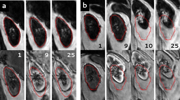
(Larger version in online supporting information. See https://onlinelibrary.wiley.com/action/downloadSupplement?doi=10.1002%2Fmrm.26999&attachmentId=203717402.) Dynamic series of two subjects, registered both to fat images (upper row) and OP images (lower row). For clarity, here the fat and OP images are shown in the upper and lower row, respectively. In red, the contour of the kidney is shown as segmented in the first dynamic. The number of the dynamic is indicated in each image. (a) Subject P4: Registration to fat images performs clearly better than registration to OP images. (b) Subject P5: Poor registration due to severe respiratory motion during the dynamic series with both techniques. OP, opposed phase; P, patient.

Registration to OP images was performed using both GCC and NMI as similarity measure. GCC‐based registration performed significantly better, resulting in a mean NRMS error of the fat time‐intensity curve of 0.08 versus 0.10 for NMI‐based registration (P = 0.005). Therefore, GCC was used as a similarity measure in the comparison with registration to fat images.

In Figure 4a, results of registration to both fat and OP images in one of the study subjects (P4) are shown. Registration to fat images resulted in good alignment of the kidney, whereas registration to OP images failed to register the kidney properly, already before CA inflow. In subject P5 (Figure 4b), registration was poor, which was explained by the severe respiratory motion during the dynamic series. This also was illustrated by a RMS vertical misalignment of 58 mm (left kidney) and 66 mm (right kidney) before registration. Overall, image quality was acceptable, although later phase images were particularly affected by motion artefacts. In Figure 5, fat time‐intensity curves are shown for four different kidneys. The curves in Figures 5a and 5b correspond to the kidneys shown in Figures 4a and 4b. Difference in registration quality in subject P4 and poor registration in subject P5 are clearly visualized.

Figure 5.

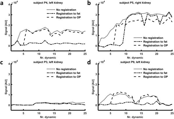
Fat time‐intensity curves for four kidneys, calculated on Dixon fat images both for registration to fat images and registration to OP images to compare performance. (In addition, the time‐intensity curve before registration is shown.) (a) The dynamic series of this kidney is shown in Figure 4a. Registration to fat images performs clearly better. (b) The dynamic series of this kidney is shown in Figure 4b. Here, both registration to fat and to OP images fail to achieve adequate alignment of the kidneys. (c) Performance of both methods is equal. (d) Although the difference is less pronounced than in (a), registration to fat performs clearly better compared to registration to OP images. Nr, number of; OP, opposed phase; P, patient.

In Figure 6, box plots of the registration errors, as measured by RMS vertical misalignment and the fat time‐intensity curve, are shown (for errors per subject, see https://onlinelibrary.wiley.com/action/downloadSupplement?doi=10.1002%2Fmrm.26999&attachmentId=203717402 in the online supporting information). Respiratory‐induced RMS vertical misalignment was calculated prior to registration as a measure for initial motion. Residual RMS vertical misalignment was calculated both after registration to fat and to OP images to allow for comparison. NRMS of the fat time‐intensity curve is given for all subjects both after registration to fat and to OP images. Respiratory‐induced motion, as measured by RMS vertical misalignment prior to registration, was 14 mm (interquartile range 13) (median over left and right kidneys over all subjects). RMS vertical misalignment was improved more by registration to fat compared to registration to OP (median 3 (3) mm vs. 5 (13) mm, respectively, P = 0.03). NRMS of the fat time‐intensity curve was smaller for registration to fat, median 0.025 (0.010) compared to 0.030 (0.095) for registration to OP images (median over left and right kidneys over all subjects, P = 0.04). Subject P5, for whom registration was poor, was excluded from further analysis.

Figure 6.

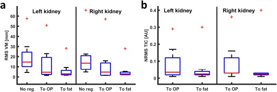
Box plots of the registration error. (a) RMS vertical misalignment before registration and after registration to OP and fat images. (b) NRMS error of the time‐intensity curve for registration to OP and to fat. In both graphs, the outlier corresponds to subject P5, in whom registration was poor. NRMS, normalized root‐mean‐square; OP, opposed phase; P, patient; RMS, root‐mean‐square; TIC, time‐intensity curve; VM, vertical misalignment.

Pharmacokinetic Model Fit

Precontrast arterial T₁ as obtained by joint estimation was 1,621 (761) ms. Estimated peak arterial contrast agent concentration was 1.0 (0.3) mM. Pharmacokinetic model fits were performed on time‐intensity curves from unregistered and fat‐ and OP‐registered images. In Figures 7a and 7b, the best and worst obtained pharmacokinetic fits are shown for registration to fat, although even the worst fit is reasonably accurate. The corresponding curves for registration to OP are shown in Figures 7c and 7d, where the curve in Figure 7c is heavily affected by motion due to suboptimal registration. Perfusion and GFR values are provided in Table 1 for all subjects except subject P5. Mean perfusion and GFR were 233 (64) mL/100 mL/min and 60 (36) mL/min (corrected for body surface area 50 (26) mL/min/1.73 m²), respectively. Mean renal volume and fractional blood volume were 172 (48) mL and 0.24 (0.10), respectively. Measured renal volume is likely an underestimation because the collecting system and partial volume artefacts were discarded during segmentation. Mean plasma transit time was 4.0 (1.4) s, with a delay of 1.9 (0.88) s. For registration to OP, mean perfusion and GFR were 265 (174) mL/100 mL/min and 84 (77) mL/min (corrected for body surface area 68 (57) mL/min/1.73 m²). Without registration, mean perfusion and GFR were 303 (190) mL/min and 83 (83) mL/min (corrected for body surface area 67 (62) mL/1.73 m²/min). For registration to OP and unregistered images, pharmacokinetic analysis yielded unphysiological values mainly in subject P9, with perfusion exceeding 500 mL/100 mL/min and skGFR exceeding 100/mL/min.

Figure 7.

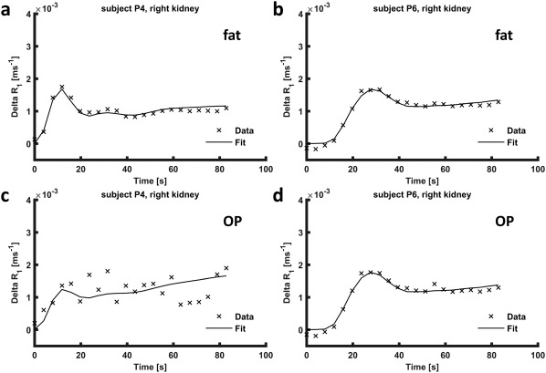
Pharmacokinetic model fits to parenchymal time‐concentration curves. (a) Subject P4, in whom the fit to the pharmacokinetic model was the worst (registration to fat). (b) Subject P6, in whom the best fit was obtained (registration to fat). (c) Time‐concentration curve of subject P4, heavily affected by motion, obtained from OP‐registered images. (d) Time‐concentration curve obtained from images registered to OP in subject P6, in whom registration to OP and to fat performed comparably. OP, opposed phase; P, patient; R₁, longitudinal relaxation rate.

Table 1.

Perfusion and GFR Values

	Perfusion						skGFR						GFRa (DCE)			eGFRb
	(mL/100 mL/min)						(mL/min)						(mL/1.73 m2/min)
	Left			Right			Left			Right			Both			Both
Reg to	–	OP	Fat	–	OP	Fat	–	OP	Fat	–	OP	Fat	–	OP	Fat	NA
P1	122	115	118	160	165	161	28	22	22	17	22	22	41	39	40	110.3
P2	174	211	225	457	790	247	18	10	9	14	13	7	32	23	16	73.1
P3	322	257	250	297	232	233	16	24	24	14	19	19	28	40	39	83.8
P4	102	3	158	97	101	152	8	9	16	7	12	10	14	20	22	67.9
P6	594	282	266	416	340	300	33	39	40	43	42	41	72	78	79	89.8
P7	181	217	211	162	230	225	75	63	64	67	60	60	109	95	95	88.5
P8	317	300	297	332	308	308	42	48	48	50	66	66	63	78	78	86.2
P9	759	597	324	608	252	349	169	149	31	122	127	29	224	212	46	78.6
P10	121	182	181	231	191	195	11	17	17	14	15	21	22	28	33	41.8
Mean	299	240	225	307	290	241	44	42	30	39	42	31	67	68	50	80.0
SD	219	152	63	156	189	64	48	41	16	35	36	20	62	57	26	18.7

Perfusion and GFR values measured using DCE MRI separate for left and right kidneys, both for registration to fat and to OP. In addition, combined GFR corrected for body surface area is calculated and shown together with GFR estimated using the CKD‐EPI formula.

^aCorrected for body surface area using the du Bois formula 35.

^bCalculated using the CKD‐EPI formula.

CKD‐EPI, chronic kidney disease epidemiology collaboration equation; DCE, dynamic contrast‐enhanced; eGFR, estimated glomerular filtration rate; GFR, glomerular filtration rate; NA, nonapplicable; OP, opposed phase; P, patient; Reg, registration; SD, standard deviation; skGFR, single kidney GFR.

Creatinine‐based eGFR is also shown in Table 1. In Figure 8, DCE‐based GFR is plotted against eGFR, and a Bland‐Altman plot of the difference is shown for registration to fat images. The correlation coefficient was 0.68 (P = 0.04), with limited agreement between the measurements as illustrated by an ICC of 0.38. For registration to OP images, the correlation coefficient was 0.55 without reaching significance (P = 0.13), and the ICC was 0.10. Without registration, the correlation coefficient was 0.58 (P = 0.10), and the ICC again was 0.10.

Figure 8.

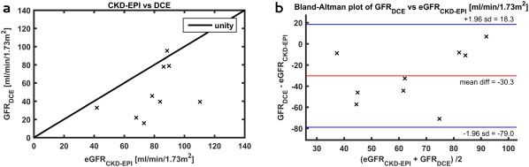
(a) DCE‐based GFR compared to eGFR estimated using the CDK‐EPI formula; (b) Bland‐Altman plot of the difference between the DCE‐based GFR and the eGFR. CKD‐EPI, chronic kidney disease epidemiology collaboration equation; DCE, dynamic contrast‐enhanced; eGFR, estimated glomerular filtration rate; GFR, glomerular filtration rate. DCE, dynamic contrast‐enhanced; eGFR, estimated glomerular filtration rate; GFR, glomerular filtration rate.

DISCUSSION

We described an approach for automated postprocessing in renal DCE MRI, which employs a new approach to image registration. Registration to Dixon fat images resulted in better registration compared to the conventional method. Furthermore, it improved the estimation of kidney perfusion and GFR, both compared to pharmacokinetic analysis without registration and analysis with registration to OP images. The proposed registration algorithm relies on the absence of contrast enhancement in fat images because gadolinium‐based CAs, which are confined to the extracellular space, do not influence the relaxation of fat protons, which are contained inside adipocytes. As expected, fat images hardly showed any contrast enhancement. Registration performed evidently better on fat images compared to OP images. However, in one subject with pronounced initial respiratory motion, registration was poor for both approaches. Presumably, this was caused by blurring of the edges of the kidney due to motion artefacts in the fat images. Contrary to our expectation, GCC‐based registration performed better than NMI‐based registration in OP images, despite visible contrast enhancement. This might be the result of the phase cancellation artefact around the kidneys, present on all dynamics regardless of the timing after contrast inflow.

Because no agreed upon measure for registration quality exists, it is difficult to make a quantitative comparison between registration algorithms. Only Merrem et al. 36 report coronal motion: the standard deviation of the vertical position of the kidney. They report an average initial coronal motion of only 3.4 mm, reducing to 1.7 mm after deformable registration, a reduction of 50%. In comparison, when we calculate this measure in our dataset, registration to fat images results in a reduction of 60%; therefore, performance of the Merrem approach seems comparable to ours. Because Merrem et al. used cross‐correlation as a similarity measure, which is sensitive to contrast changes during CA inflow, registration could likely be improved further by registration to Dixon fat images.

Others 19, 20, 37 proposed registration algorithms based on MI. However, they all used a preregistration module before MI‐based registration. Consequently, our method will be easier to implement. Other groups used approaches based on edge detection 8, 10, 15, 16, 17, 18, yielding good results without requiring preregistration modules. However, implementation of the algorithms might be challenging in clinical practice, whereas the registration algorithm we used is freely available. In addition, postprocessing is automated in a graphical user interface and therefore does not require specialist knowledge. Only for segmentation is manual interaction required to adjust the fat threshold (optionally), set the number of clusters, and label the resultant masks.

In the aorta, calculation of CA concentration could be improved by implementation of the approach recently proposed by Simonis et al. 38. Here, the complex signal is used instead of magnitude alone. In large vessels parallel to the direction of the static (B₀) field, signal phase proves to be linearly related to CA concentration. In addition, this approach can correct for spatial inhomogeneity of the radiofrequency (B₁) field, which we could not correct for. This is less relevant on 1.5 T because B₁ inhomogeneity is limited but must be accounted for when moving to higher field strengths. In this analysis, this approach could not be implemented because the source images were not available.

Fitting of the Toft renal two‐compartment model yielded a mean cortical perfusion of 233 mL/100 mL/min for fat‐registered images. The values obtained using fat‐registered images are in good agreement with other renal DCE MRI studies, whereas unregistered and OP‐registered images yielded unphysiological values in some kidneys. Sourbron et al. 33 report a perfusion of 229 mL/100 mL/min, calculated with an instantaneous exponential VIRF. Tofts et al. 34 report a renal flow of 465 mL/100 mL/min, calculated with a delayed exponential VIRF. The hypertensive population in our study probably explains the relative low perfusion because renal vascular resistance is known to be increased in hypertensive subjects 39. Correlation between eGFR based on creatinine clearance and GFR measured using DCE MRI was significant when fat‐registered images were used, although agreement was limited (ICC of 0.38). This is worse compared to results reported recently by Eikefjord et al. 40, who found an ICC of 0.49 in living kidney donors. In nephrectomized subjects, Tipirneni‐Sajja et al. 41 found comparable results for DCE MR‐based GFR measurement. However, both authors compared MR‐based GFR to reference standard methods of GFR measurement: iohexol and ^99mTC‐DTPA clearance, respectively. Very good agreement between DCE‐based GFR and creatinine‐based GFR was reached by Pandey et al. 42. They used a golden angle stack‐of‐stars approach for data acquisition. From eight different image reconstruction schemes, one resulted in < 5% discrepancy between the DCE‐based and creatinine‐based approach. However, creatinine‐based GFR provides only a crude estimate of actual GFR. For example, the CKD‐EPI formula yields an eGFR within 10% of the value measured using the reference standard (inulin, iohexol, or iothalamate clearance) only for less than 45% of the subjects 43. According to the same study, it overestimates the GFR in healthy adults on average by more than 10%. In contrast, the Tofts model gives an underestimation of the GFR, which was expected to be about 20 mL/100 mL/min according to the simulations in the supporting information. This presumably explains the large mean difference between creatinine‐based eGFR and MR‐based GFR in our study, which is clearly visualized in the Bland‐Altman plot in Figure 8b. Furthermore, the time delay between measurement of the creatinine level and the MRI might be a possible explanation for the limited agreement between creatinine‐based eGFR and MR‐based GFR. Biological variation of creatinine clearance is considerable, with a standard deviation of about 12% for repeated measurements 44. Nevertheless, our DCE protocol can be improved. Most importantly, both the temporal resolution and the duration of measurement must be increased. The limited temporal resolution and measurement duration prevents us from using the Sourbron model 33. This model is physiologically more accurate because it also models tubular outflow. The simulations in the supporting information show this model indeed yields more accurate results compared to the Tofts model. Furthermore, separate analysis for the cortex and medulla can easily be implemented because separate masks already are generated using the k‐means clustering approach. Because filtration only occurs in the glomeruli in the cortex, this will likely result in improved accuracy of the GFR measurement. In addition, it enables voxelwise analysis to construct perfusion and filtration maps of the kidney, possibly demonstrating focal differences in renal perfusion and function.

Limitations

A drawback of our method is the increase in DCE acquisition time inherent to the acquisition of dual‐echo images. Despite this, we still managed to achieve a temporal resolution of less than 4 seconds, as recommended by Michaely et al. 12. The relatively long acquisition time for 3D acquisition results in more pronounced respiratory motion artefacts in the images; however, on the fat images, motion artefacts seem to disturb the contour of the kidney less when compared to OP images, presumably due to the great contrast between the kidney and the surrounding adipose tissue. The temporal resolution can easily be decreased by moving to 3T because the twofold increase in the Larmor frequency, and hence in the water–fat shift, in principle allows for a twofold decrease in echo time. In addition, parallel imaging performance is better at 3T.

Only rigid registration was performed because craniocaudal translation is the dominant motion during respiration in the kidneys. Furthermore, the added value of nonrigid registration is not clear 15, 45, whereas it does result in increased computational time.

Unfortunately, hematocrit values were not available for most subjects; therefore, we had to assume a fixed value for large vessel hematocrit. Likely, perfusion estimates can be improved when incorporating individual hematocrit values 34.

CONCLUSION

We have demonstrated the feasibility of automated postprocessing in renal DCE MRI. To handle respiratory motion, one of the main challenges in renal DCE MRI, image registration to fat images was employed. Registration quality was superior to registration to OP images, thanks to negligible contrast enhancement in fat images. The method was robust, being able to register nine out of 10 images in a satisfactory manner. Because manual interaction was limited, postprocessing does not require specialist knowledge. Therefore, it will be easy to implement in clinical practice. A drawback of this method is the cost in imaging time, resulting in a temporal resolution of 3.9 s; however, straightforward reduction in dynamic imaging time can be achieved by migrating to 3T. After implementation of the improvements mentioned in the discussion, the next step will be to validate the GFR obtained using this renal DCE‐MRI protocol in healthy volunteers compared to a reference standard such as inulin clearance.

Supporting information

Additional supporting information may be found in the online version of this article.

Fig. S1. Example of tissue‐concentration curve and AIF (generic AIF as modelled by Parker et al. (S3)) used for determination of fit accuracy. In solid lines the high resolution curve is depicted, the sampling points denote the measurements in our MR sequence. Sample points: dt 3.94 s, tmax 98.5 s.

Fig. S2. Comparison of perfusion and GFR estimated using Sourbron's and Tofts’ models. The shaded area denotes 1.96 times the standard deviation. The black horizontal line denotes true perfusion or GFR and the dotted black vertical lines denote dt and t_max of our data (3.94 s and 98.5 s, respectively); a) dependence of perfusion estimation on decreasing temporal resolution (or increasing dt on the x‐axis); b) GFR dependence on temporal resolution; c) estimation of perfusion, dependence on duration of measurement (t_max) and d) the same for GFR.

Fig. S3. a) Normalized variance $\left(\sqrt{\frac{Var\left(x\right)}{{\mathrm{\mu }}_x^2}}\right)$ of T_t (tubular transit time) and the other fit parameters versus measurement time. Note that the variance of T_t exceeds the variance of the other parameters by far; b) normalized covariance $\left(\sqrt{\frac{Var\left(xy\right)}{{\mathrm{\mu }}_x{\mathrm{\mu }}_y}}\right)$ of T_t with the other parameters as a function of measurement time.

Fig. S4. Full version of figure 4 in the main text. Dynamic series of two subjects, registered both to fat‐images (upper row) and OP images (lower row). For clarity, here the fat and OP images are shown in the upper and lower row, respectively. In red, the contour of the kidney is shown as segmented on the first dynamic. The number of the dynamic is indicated on each image; a) subject P4: registration to fat‐images performs clearly better than registration to OP images; b) subject P5: poor registration due to severe respiratory motion during the dynamic series with both techniques.

Table S1. Quantitative registration results. Respiratory induced RMS vertical misalignment for all subjects before and after registration to OP and fat‐images are depicted. Normalized RMS error of the time‐intensity curve of the fat‐image only was calculated after registration, to allow comparison between registration to fat and OP images. In almost every subject, registration to fat results in smaller errors than registration to OP.

REFERENCES

- 1. Zöllner FG, Zimmer F, Klotz S, Hoeger S, Schad LR. Renal perfusion in acute kidney injury with DCE‐MRI: deconvolution analysis versus two‐compartment filtration model. Magn Reson Imaging 2014;32:781–785. [DOI] [PubMed] [Google Scholar]
- 2. Buckley DL, Shurrab AE, Cheung CM, Jones AP, Mamtora H, Kalra PA. Measurement of single kidney function using dynamic contrast‐enhanced MRI: comparison of two models in human subjects. J Magn Reson Imaging 2006;24:1117–1123. [DOI] [PubMed] [Google Scholar]
- 3. Chapman SJ, Wah TM, Sourbron SP, Buckley DL. The effects of cryoablation on renal cell carcinoma perfusion and glomerular filtration rate measured using dynamic contrast‐enhanced MRI: a feasibility study. Clin Radiol 2013;68:887–894. [DOI] [PubMed] [Google Scholar]
- 4. Eikefjord E, Andersen E, Hodneland E, Zollner F, Lundervold A, Svarstad E, Rorvik J. Use of 3D DCE‐MRI for the estimation of renal perfusion and glomerular filtration rate: an intrasubject comparison of FLASH and KWIC with a comprehensive framework for evaluation. AJR Am J Roentgenol 2015;204:W273–W281. [DOI] [PubMed] [Google Scholar]
- 5. Notohamiprodjo M, Sourbron S, Staehler M, et al. Measuring perfusion and permeability in renal cell carcinoma with dynamic contrast‐enhanced MRI: a pilot study. J Magn Reson Imaging 2010;31:490–501. [DOI] [PubMed] [Google Scholar]
- 6. Notohamiprodjo M, Staehler M, Steiner N, Schwab F, Sourbron SP, Michaely HJ, Helck AD, Reiser MF, Nikolaou K. Combined diffusion‐weighted, blood oxygen level‐dependent, and dynamic contrast‐enhanced MRI for characterization and differentiation of renal cell carcinoma. Acad Radiol 2013;20:685–693. [DOI] [PubMed] [Google Scholar]
- 7. Wang W, Ding J, Li Y, Wang C, Zhou L, Zhu H, Peng W. Magnetic resonance imaging and computed tomography characteristics of renal cell carcinoma associated with Xp11.2 translocation/TFE3 gene fusion. PLoS One 2014;9:e99990. [DOI] [PMC free article] [PubMed] [Google Scholar]
- 8. Khalifa F, El‐Baz A, Gimel'farb G, Abu El‐Ghar M. Non‐invasive image‐based approach for early detection of acute renal rejection. Med Image Comput Comput Assist Interv 2010;13:10–18. [DOI] [PubMed] [Google Scholar]
- 9. Khalifa F, Abou El‐Ghar M, Abdollahi B, Frieboes HB, El‐Diasty T, El‐Baz A. A comprehensive non‐invasive framework for automated evaluation of acute renal transplant rejection using DCE‐MRI. NMR Biomed 2013;26:1460–1470. [DOI] [PubMed] [Google Scholar]
- 10. Liu W, Sung K, Ruan D. Shape‐based motion correction in dynamic contrast‐enhanced MRI for quantitative assessment of renal function. Med Phys 2014;41:122302. [DOI] [PMC free article] [PubMed] [Google Scholar]
- 11. Dujardin M, Sourbron S, Luypaert R, Verbeelen D, Stadnik T. Quantification of renal perfusion and function on a voxel‐by‐voxel basis: a feasibility study. Magn Reson Med 2005;54:841–849. [DOI] [PubMed] [Google Scholar]
- 12. Michaely HJ, Sourbron SP, Buettner C, Lodemann KP, Reiser MF, Schoenberg SO. Temporal constraints in renal perfusion imaging with a 2‐compartment model. Invest Radiol 2008;43:120–128. [DOI] [PubMed] [Google Scholar]
- 13. Palmowski M, Schifferdecker I, Zwick S, Macher‐Goeppinger S, Laue H, Haferkamp A, Kauczor HU, Kiessling F, Hallscheidt P. Tumor perfusion assessed by dynamic contrast‐enhanced MRI correlates to the grading of renal cell carcinoma: initial results. Eur J Radiol 2010;74:e176–e180. [DOI] [PubMed] [Google Scholar]
- 14. Attenberger UI, Sourbron SP, Michaely HJ, Reiser MF, Schoenberg SO. Retrospective respiratory triggering renal perfusion MRI. Acta Radiol 2010;51:1163–1171. [DOI] [PubMed] [Google Scholar]
- 15. Zikic D, Sourbron S, Feng X, Michaely HJ, Khamene A, Navab N. Automatic alignment of renal DCE‐MRI image series for improvement of quantitative tracer kinetic studies. In Proceedings of SPIE 6914, Medical Imaging: Image Processing, San Diego, California, USA, 2008. p. 32.
- 16. de Senneville BD, Mendichovszky IA, Roujol S, Gordon I, Moonen C, Grenier N. Improvement of MRI‐functional measurement with automatic movement correction in native and transplanted kidneys. J Magn Reson Imaging 2008;28:970–978. [DOI] [PubMed] [Google Scholar]
- 17. Song T, Lee VS, Rusinek H, Kaur M, Laine AF. Automatic 4‐D registration in dynamic MR renography based on over‐complete dyadic wavelet and Fourier transforms. Med Image Comput Comput Assist Interv 2005;8:205–213. [DOI] [PubMed] [Google Scholar]
- 18. Yang X, Ghafourian P, Sharma P, Salman K, Martin D, Fei B. Nonrigid registration and classification of the kidneys in 3D dynamic contrast enhanced (DCE) MR images. Proc SPIE Int Soc Opt Eng 2012;8314:83140B. [DOI] [PMC free article] [PubMed] [Google Scholar]
- 19. Zöllner FG, Sance R, Rogelj P, Ledesma‐Carbayo MJ, Rørvik J, Santos A, Lundervold A. Assessment of 3D DCE‐MRI of the kidneys using non‐rigid image registration and segmentation of voxel time courses. Comput Med Imaging Graph 2009;33:171–181. [DOI] [PubMed] [Google Scholar]
- 20. Positano V, Bernardeschi I, Zampa V, Marinelli M, Landini L, Santarelli MF. Automatic 2D registration of renal perfusion image sequences by mutual information and adaptive prediction. Magn Reson Mater Phy 2013;26:325–335. [DOI] [PubMed] [Google Scholar]
- 21. Hodneland E, Hanson EA, Lundervold A, Modersitzki J, Eikefjord E, Munthe‐Kaas AZ. Segmentation‐driven image registration‐ application to 4D DCE‐MRI recordings of the moving kidneys. IEEE Trans Image Process 2014;23:2392–2404. [DOI] [PubMed] [Google Scholar]
- 22. Hodneland E, Lundervold A, Rorvik J, Munthe‐Kaas AZ. Normalized gradient fields for nonlinear motion correction of DCE‐MRI time series. Comput Med Imaging Graph 2014;38:202–210. [DOI] [PubMed] [Google Scholar]
- 23. Cheng KT. Gadobutrol. Molecular Imaging and Contrast Agent Database (MICAD). National Center for Biotechnology Information (US). Available at: https://www.ncbi.nlm.nih.gov/books/NBK23589/. Published February 15, 2006. Updated October 18, 2007. Accessed September 8, 2017.
- 24. Vink EE, De Boer A, Hoogduin HJM, Voskuil M, Leiner T, Bots ML, Joles JA, Blankestijn PJ. Renal BOLD‐MRI relates to kidney function and activity of the renin‐angiotensin‐aldosterone system in hypertensive patients. J Hypertens 2015;33:597–604. [DOI] [PubMed] [Google Scholar]
- 25. Levey AS, Stevens LA, Schmid CH, et al. A new equation to estimate glomerular filtration rate. Ann Intern Med 2009;150:604–612. [DOI] [PMC free article] [PubMed] [Google Scholar]
- 26. Eggers H, Brendel B, Duijndam A, Herigault G. Dual‐echo Dixon imaging with flexible choice of echo times. Magn Reson Med 2011;65:96–107. [DOI] [PubMed] [Google Scholar]
- 27. Hartkens T, Rueckert D, Schnabel JA, Hawkes DJ, Hill DLG. VTK CISG registration toolkit an open source software package for affine and non‐rigid registration of single‐ and multimodal 3D images. In: Proceedings of the Workshop Bildverarbeitung für die Medizin, Leipzig, Germany, 2002. p. 409–412.
- 28. Pluim JPW, Maintz JBA, Viergever MA. Mutual‐information‐based registration of medical images: a survey. IEEE Trans Med Imaging 2003;22:986–1004. [DOI] [PubMed] [Google Scholar]
- 29. O'Leary DP, Rust BW. Variable projection for nonlinear least squares problems. Comput Optim Appl 2012;54:579–593. [Google Scholar]
- 30. Golub G, Pereyra V. Separable nonlinear least squares: the variable projection method and its applications. Inverse Problems 2003;19:R1. [Google Scholar]
- 31. Dickie BR, Banerji A, Kershaw LE, McPartlin A, Choudhury A, West CM, Rose CJ. Improved accuracy and precision of tracer kinetic parameters by joint fitting to variable flip angle and dynamic contrast enhanced MRI data. Magn Reson Med 2016;76:1270–1281. [DOI] [PubMed] [Google Scholar]
- 32. Teixeira RP, Malik SJ, Hajnal JV. Joint system relaxometry (JSR) and Cramer‐Rao lower bound optimization of sequence parameters: a framework for enhanced precision of DESPOT T1 and T2 estimation. Magn Reson Med 2018;79:234–245. [DOI] [PMC free article] [PubMed] [Google Scholar]
- 33. Sourbron SP, Michaely HJ, Reiser MF, Schoenberg SO. MRI‐measurement of perfusion and glomerular filtration in the human kidney with a separable compartment model. Invest Radiol 2008;43:40–48. [DOI] [PubMed] [Google Scholar]
- 34. Tofts PS, Cutajar M, Mendichovszky IA, Peters AM, Gordon I. Precise measurement of renal filtration and vascular parameters using a two‐compartment model for dynamic contrast‐enhanced MRI of the kidney gives realistic normal values. Eur Radiol 2012;22:1320–1330. [DOI] [PubMed] [Google Scholar]
- 35. Du Bois D, Du Bois EF. A formula to estimate the approximate surface area if height and weight be known. 1916. Nutrition 1989;5:303–311; discussion 312–313. [PubMed] [Google Scholar]
- 36. Merrem AD, Zollner FG, Reich M, Lundervold A, Rorvik J, Schad LR. A variational approach to image registration in dynamic contrast‐enhanced MRI of the human kidney. Magn Reson Imaging 2013;31:771–777. [DOI] [PubMed] [Google Scholar]
- 37. Sance R, Ledesma‐Carbayo MJ, Lundervold A, Santos A. Alignment of 3D DCE‐MRI abdominal series for optimal quantification of kidney function. In: Proceedings of the 5th International Symposium on Image and Signal Processing and Analysis, Istanbul, Turkey, 2007. p. 413–417.
- 38. Simonis FF, Sbrizzi A, Beld E, Lagendijk JJ, van den Berg CA. Improving the arterial input function in dynamic contrast enhanced MRI by fitting the signal in the complex plane. Magn Reson Med 2016;76:1236–1245. [DOI] [PubMed] [Google Scholar]
- 39. Pedersen EB, Kornerup HJ. Renal haemodynamics and plasma renin in patients with essential hypertension. Clin Sci Mol Med 1976;50:409–414. [DOI] [PubMed] [Google Scholar]
- 40. Eikefjord E, Andersen E, Hodneland E, Svarstad E, Lundervold A, Rorvik J. Quantification of single‐kidney function and volume in living kidney donors using dynamic contrast‐enhanced MRI. AJR Am J Roentgenol 2016:207:1022–1030. [DOI] [PubMed] [Google Scholar]
- 41. Tipirneni‐Sajja A, Loeffler RB, Oesingmann N, Bissler J, Song R, McCarville B, Jones DP, Hudson M, Spunt SL, Hillenbrand CM. Measurement of glomerular filtration rate by dynamic contrast‐enhanced magnetic resonance imaging using a subject‐specific two‐compartment model. Physiol Rep 2016;4:e12755. [DOI] [PMC free article] [PubMed] [Google Scholar]
- 42. Pandey A, Yoruk U, Keerthivasan M, Galons JP, Sharma P, Johnson K, Martin DR, Altbach MI, Bilgin A, Saranathan M. Multiresolution imaging using golden angle stack‐of‐stars and compressed sensing for dynamic MR urography. J Magn Reson Imaging 2017;46:303–311. [DOI] [PMC free article] [PubMed] [Google Scholar]
- 43. Pottel H, Hoste L, Dubourg L, et al. An estimated glomerular filtration rate equation for the full age spectrum. Nephrol Dial Transplant 2016;31:798–806. [DOI] [PMC free article] [PubMed] [Google Scholar]
- 44. Greenblatt DJ, Ransil BJ, Harmatz JS, Smith TW, Duhme DW, Koch‐Weser J. Variability of 24‐hour urinary creatinine excretion by normal subjects. J Clin Pharmacol 1976;16:321–328. [DOI] [PubMed] [Google Scholar]
- 45. Rogelj P, Zoellner FG, Kovačič S, Lundervold A. Motion correction of contrast‐enhanced MRI time series of kidney. In: Proceedings of the 16th International Electrotechnical and Computer Science Conference, Portoroz, Slovenia, 2007. p. 191–194.
Associated Data
This section collects any data citations, data availability statements, or supplementary materials included in this article.
Supplementary Materials