Bridging observational studies and randomized experiments by embedding the former in the latter

Abstract

Consider a statistical analysis that draws causal inferences from an observational dataset, inferences that are presented as being valid in the standard frequentist senses; i.e. the analysis produces: (1) consistent point estimates, (2) valid p-values, valid in the sense of rejecting true null hypotheses at the nominal level or less often, and/or (3) confidence intervals, which are presented as having at least their nominal coverage for their estimands. For the hypothetical validity of these statements, the analysis must embed the observational study in a hypothetical randomized experiment that created the observed data, or a subset of that hypothetical randomized data set. This multistage effort with thought-provoking tasks involves: (1) a purely conceptual stage that precisely formulate the causal question in terms of a hypothetical randomized experiment where the exposure is assigned to units; (2) a design stage that approximates a randomized experiment before any outcome data are observed, (3) a statistical analysis stage comparing the outcomes of interest in the exposed and non-exposed units of the hypothetical randomized experiment, and (4) a summary stage providing conclusions about statistical evidence for the sizes of possible causal effects. Stages 2 and 3 may rely on modern computing to implement the effort, whereas Stage 1 demands careful scientific argumentation to make the embedding plausible to scientific readers of the proffered statistical analysis. Otherwise, the resulting analysis is vulnerable to criticism for being simply a presentation of scientifically meaningless arithmetic calculations. The conceptually most demanding tasks are often the most scientifically interesting to the dedicated researcher and readers of the resulting statistical analyses. This perspective is rarely implemented with any rigor, for example, completely eschewing the first stage. We illustrate our approach using an example examining the effect of parental smoking on children’s lung function collected in families living in East Boston in the 1970s.

1 Introduction

The norm in many biomedical fields, especially in environmental epidemiology, is to report associations between exposures and health outcomes using standard regression models analyzing non-randomized data^1–3 often because of ethical or logistic concerns about enforcing randomized assignment. However, causal relationships between exposures and outcomes characterizing human health, although more difficult to estimate than associations, are always the actual estimands in biomedical research, and moreover, estimates of these effects are expected by readers of journals interested in policy implications. Here we consider an approach that estimates explicitly the causal effects of parental smoking on children’s lung function, a causal question that is important, yet unanswered by extant analyses because past epidemiological studies have reported discordant estimates.⁴ Providing accurate estimates of the causal effects of children’s exposure to parental smoking is crucial to risk assessors. Although our analytic approach does not directly address the effects of specific interventions to curtail parental smoking, it does implicitly suggest, in the fourth stage, possible interventions to reduce the consequences on health outcomes. The causal versus associational nature of this relationship is reflected by the assertion that no matter what pre-assignment background characteristics lead to children’s exposure to smoking parents in the observed data set, excess morbidity among the exposed would have been reduced if preventative interventions were implemented; the related assertion is that analogous results will be observed in the future.

The general framework that we consider in this paper is sometimes called the “Rubin Causal Model”^5–8 for work done in the 1970s. This approach using potential outcomes to define causal effects was originally proposed by Neyman in 1923⁹ but its use was restricted to randomized experiments until Rubin extended it to define causal effects in general.¹⁰ To address causality, the key insight is to (multiply) impute the missing potential outcomes for each unit, i.e. what the outcome would have been under the other (meaning, not taken) treatment. In contrast, most published epidemiological studies model only the observed outcome data (i.e. not the potential outcomes) using associational models implicitly assuming that “association implies some sort of causation.”¹¹ The main focus of this manuscript is to illustrate how to incorporate conceptual and design stages in observational studies prior to any analysis stage examining outcome data, which follows previous logic proposed by Rubin.^12,13 Our approach transports established insights from classical experimental design, which revolutionized many empirical fields from 1925 to 1960.^14–17 Specifically, we use design strategies that were suggested in the late 1960s and early 1970s,^18–21 and compare the results to the results obtained by the standard strategy used in environmental epidemiology.

2 Our suggested approach – steps towards statistical evidence

Consider the specific environmental health example to estimate the causal effect of exposure to one factor, parental smoking, on children’s lung function, assessed using forced expiratory volume in one second (FEV-1) in children using data collected in East Boston in the 1970s and previously analyzed decades ago²² and more recently used for pedagogical purposes.²³ From our perspective, most reports analyzing these data lacked both a conceptual stage and a design stage, and focused on the conclusions based on standard regressions generated from a simple analysis stage.

2.1 The standard analysis stage strategy

The standard epidemiological approach to such data has lung function as the outcome variable and has parental smoking and background variables as predictors in generalized linear or additive regression models. Association estimates are obtained, but:

1. Are these estimated effects of similar magnitude to those that would be obtained if the researcher had conducted a real randomized experiment? Note that the randomized experiment is not uniquely defined in this context.

2. What are the assumptions underlying standard regression models and are they straightforward or opaque?

3. What are the precise meanings and robustness of the reported statistical summaries (e.g. uncertainties, interval estimates, p-values)?

2.2 Objective and valid causal inference under stated assumptions

In contrast, we propose a strategy with four transparent, distinct, and ordered stages, following implicit advice in classical texts on experimental design (e.g. Fisher,^14,15 Kempthorne,¹⁶ Cochran and Cox,¹⁷ Box et al.²⁴) and a more recent text extending this perspective to non-randomized studies.⁸

1. A conceptual stage that involves the precise formulation of the causal question (and related assumptions) using potential outcomes and described in terms of a hypothetical randomized experiment in which the exposure is randomly assigned to units; this description includes the timing of assignment and defines the target population; no computation is needed at this stage, but rather careful thought and argumentation.

2. A design stage that attempts to reconstruct (or approximate) the design of a randomized experiment before any outcome data are observed (i.e. with unconfounded assignment of exposure using the observed background and treatment assignment data); typically, heavy use of computing is needed at this stage, e.g. for multivariate matched sampling and extensive balance diagnostics.

3. A statistical analysis stage defined in a protocol explicated before seeing any outcome data, comparing the outcomes of interest in similar (e.g., hypothetically randomly divided) exposed and non-exposed units of the hypothetical randomized experiment; this stage is the one that most closely parallels the standard model-based analyses but uses more flexible methods. The predefined protocol is crucial to prevent extensive model selection based on hunting for significant “p-values”.

4. A summary stage providing conclusions about statistical evidence for the sizes of possible causal effects of the exposure; no computing is required at this stage, just thoughtful summarization, e.g. focusing on what actual world interventions could be implemented to curtail any untoward causal effects of the exposure.

3 Our illustrative application: the effect of parental smoking on children’s lung function

Our data set comprises 654 children and young adults, 318 females and 336 males, with 10% having parents who smoke. The children’s ages range between 3 and 19. Regarding the heights of the children, the mean is 61 inches and they range between 46 and 74 inches.

3.1 Overview of the four stages in our example

3.1.1 Conceptual stage: precise formulation of the causal question

Various hypothetical randomized experiments in which “enforced smoking cessation” is randomly assigned to parents, can be conceptualized (e.g. Bernouilli trial, completely randomized experiment, stratified randomized experiment, paired randomized experiment). At this initial stage, the plausibility of the reconstructed hypothetical randomization is important because we want to convince the reader of that position on which the entire analysis is formally predicated. Different timings of the random assignment can be imagined (e.g. before or after conception of the child) and different target populations from which the sample of 654 children was drawn can be considered.

3.1.2 Design phase: reconstruction of the hypothetical experiment

To address causality, we start by approximating the ideal conditions of a randomized experiment, which demands unconfounded assignment of exposure given observed covariates. Unconfoundedness of the exposure’s assignment can be achieved approximately by matching that aims to create exchangeable groups (e.g. strata, pairs) of exposed (to parental smoking) and non-exposed units with randomly different values of pre-exposure (background) covariates. In this simplified example, such covariates include age, height, and sex, because these variables are recorded in the existing data set. We will see that this effort is not as trivial conceptually as we might hope, as discussed shortly. That is, we attempt to create exchangeable exposed and unexposed groups or matched pairs of children, one member (or part) of each group or pair is randomly assigned to smoking parents and the other member to non-smoking parents but matched on age, height, and sex. Some earlier methods and associated theory are summarized by Rubin²¹ and Rosenbaum,²⁵ and more recent approaches are given in Sekhon²⁶ and Hansen et al.²⁷ If the matching strategy creating two such identical groups or pairs of children is entirely successful, there can be no confounding with respect to the background variables that we used for matching. It is obviously not ethical to transfer children to different parents, but perhaps it is plausible that non-smoking characteristics of smoking and non-smoking parents have no effect on children’s lung function. At least we should be explicit about such important, but typically implicit, assumptions.

Another important issue related to the timing of the observational data collection arises in this setting because children’s characteristics (such as age, height, and sex) in our data set are actually known only a posteriori, that is, after assignment to the exposure. If we assess whether children are similar with respect to variables measured after the assignment of exposure, we need to assume, for the validity of simple analyses, that these variables are not affected by the exposure. Note that this assumption implies that the height of each child with smoking parents was not affecting by parental smoking exposure. Although we found no evidence against parental smoking influencing height in this data set after applying our suggested approach but considering height as an outcome with age and sex as covariates, a French longitudinal cohort study suggests that this assumption may not be valid.²⁸

3.1.3 Analysis phase

We start by using computationally flexible techniques, such as statistical matching, to achieve balanced distributions of the background variables in the exposed and unexposed children. The most straightforward analysis examines the difference in lung function between the exposed children and the unexposed children, and these are then averaged over all children to obtain an estimate of the average causal effect. Randomization-based inference can be conducted using modern computing techniques⁸ to test the sharp null hypothesis that exposure to parental smoking has absolutely no effect, relative to no smoking exposure, on children’s lung function. Frequentist or Bayesian regression models can also be used at that stage in order to increase efficiency, by removing residual confounding that was not adequately addressed during the design stage, e.g. allowing treated and controls to have separate regression slopes and separate residual variances.^{19–21,29,30} It is critical that the analysis stage needs to be specified in a protocol explicated before seeing any outcome data.

3.1.4 Causal conclusion

If one observes a significant difference in average lung function outcome between these exchangeable groups or matched pairs (i.e. a difference that would be a rare event in the hypothetical randomized experiment if there were no effect of exposure), it is natural to attribute that difference to the differential exposures to parental smoking, and critically, to propose that the negative effect could be ameliorated by the introduction of some hypothetical intervention to curtail smoking, yet to be debated.

3.2 Details of the three first stages in our example

3.2.1 Six hypothetical experiments (first stage)

Various possible randomized interventions to curtail parental smoking are now discussed.

Hypothetical experiment A: One hypothetical completely randomized experiment (with N_Smoking = 65 children with smoking parents and N_Non-smoking = 589 children with non-smoking parents) involves intervening on smoking households before they have children and randomizing them to stop smoking with probability 9/10, and thus with probability 1/10 to continue to smoke.

Formulating a hypothetical intervention can be challenging. First, it should be plausible enough to convince readers to continue reading. However, we believe it is one of the most interesting and scientifically, not mathematically, relevant steps for epidemiological researchers. Note that whatever hypothetical intervention you posit for the experiment underlying your dataset, you are assuming that you will obtain essentially the same analytic answer for all versions of that hypothetical experiment. That is, there is a hidden assumption at this stage that, whichever version of the hypothetical intervention you choose, it will lead to approximately the same estimated causal effect. More precisely, in our example, can you argue that the hypothetical intervention assuming that the population consisted of only smoking parents who were assigned to stop smoking with probability 9/10 (and they all complied) would lead to the same conclusion as if the population consisted of only non-smoking parents who were assigned to smoke with probability 1/10 with full compliance? The latter would be clearly unethical considering what we now know about smoking exposure. But this question emphasizes the type of question you should be willing to entertain and answer. Actually, we do not consider Hypothetical Experiment A plausible. For reason discussed shortly, perhaps discarding unexposed children with background characteristics that are unlike the exposed children and vice versa would improve the plausibility of a hypothetical experiment.

Hypothetical experiment B: Another hypothetical completely randomized experiment could have resulted in exposed children with background covariates that are within the range of the background covariates of the unexposed children, and unexposed children with background covariates that are within the range of the background covariates of the exposed children. That is, suppose we selected boundaries for the covariates age and height, and restricted the 361 children to fall within those boundaries. This strategy led to N_Smoking = 61 children with smoking parents and N_Non-smoking = 300 children with non-smoking parents. At this point, an underlying hypothetical experiment that generated the data was not yet considered plausible; the specific reasons will be explained in section 3.2.4.

Hypothetical experiment C: Another hypothetical randomized experiment could have resulted in non-smoking parents with background covariates that are within certain strata defined by the background covariates of the smoking parents. This formulation is described more precisely in Section 3.2.2, part b), and led to N_Smoking = 57 children with smoking parents and N_Non-smoking = 216 children with non-smoking parents.

Other hypothetical randomized experiments would also intervene on smoking parents before their child’s conception; we describe two such experiments. First, Hypothetical experiment D.1, a completely randomized experiment with balanced groups (e.g. creating two equal-sized groups of parents similar on background characteristics, that is, N_Smoking = N_Non-smoking = 63 children). Or second, Hypothetical experiment D.2, a rerandomized experiment with two equal-sized groups of similar parents (with N_Smoking = N_Non-smoking = 63) for which the randomized allocations are allowed only when parents’ covariates (e.g. height) mean differences between smokers and non-smokers are within some a priori defined calipers.

Another hypothetical randomized experiment, Hypothetical experiment E, would intervene after the child’s conception, from the point in time for which we know the child’s sex, and would have a paired-randomized experiment where a coin flip determines which parents of a pair of two similar parents expecting a child with same sex is exposed to still-smoking parents, with N_Smoking = N_Non-smoking = 63 children).

We define the “finite population” as the population being randomized in each of the reconstructed hypothetical experiments. The super-population is a hypothetical “infinite population” from which the finite population is drawn.

3.2.2 Several different design phase strategies (second stage)

(a) No design stage (a)

The standard approach in environmental epidemiological lacks both a conceptual stage and a design stage and simply focuses on associations gleaned from observed data (N_children = 654).

(b) Trimming (b)

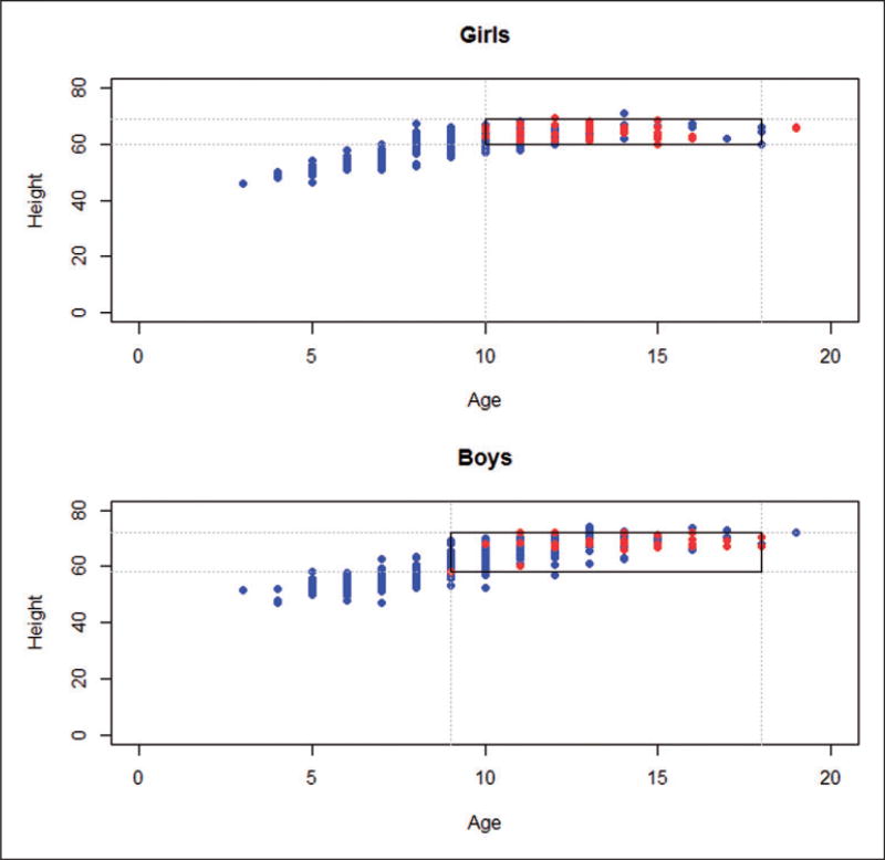
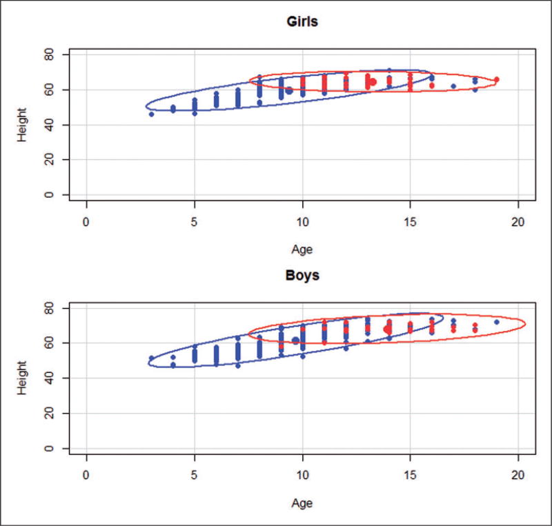
A relatively naïve strategy attempts to eliminate units from one group (i.e. treated or control) outside the range of the other group with respect to background covariates by trimming “outlier” units. To restrict imbalance with respect to age and height in the exposed vs. non-exposed groups, we included girls with ages between 10 and 18 and heights between 60 and 69 inches, and included boys with ages between 9 and 18 and heights between 58 and 72 inches; these restrictions leave us with 361 units out of 654 (see Figure 1). An alternative to trimming with rectangle boundaries could involve trimming outside the overlap of the ellipses of the bivariate distributions of the girls with smoking parents vs. girls with non-smoking parents and similarly for boys (see Figure 2), which is another example of an “intersection” matching method,³¹ but we will only consider rectangular intersection trimming in the following sections of the paper. Note that, after the trimming stage, any remaining imbalance in any background variable (e.g. age) between the exposed and non-exposed groups still limits our ability to assert that the “hypothetically randomized” exposure was the sole reason for the lack of balanced background covariates between children with smoking parents and children with non-smoking parents.

Figure 1.

Trimming approach with rectangle boundaries for age and height.

Figure 2.

Trimming with ellipsoidal boundaries for age and height.

(c) Stratified matching (c)

Another approach goes beyond trimming and construct discretized covariates and thus strata in which these discretized background covariates are balanced. This strategy, essentially proposed decades ago in the context of imputing missing data through “hot deck” imputation,³² and then for matching in causal inference by Cochran,¹⁸ has recently become popularized and renamed “coarsened exact matching.”³³ This approach eliminated 381 children out of 654.

(d) Propensity score one-to-one matching after overlap assessment and discarding (d)

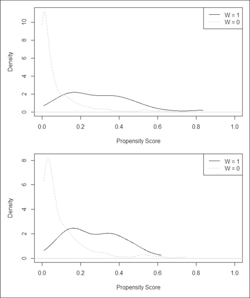
A one-to-one matching strategy with calipers³⁴ on the estimated propensity score,²⁵ for instance estimated by a logistic regression that regresses parental smoking on the available covariates in the dataset (e.g. age, height, sex, and nonlinear functions of them), but no outcome variables, can also be used in the design stage. A more parsimonious (and therefore simpler to interpret) model including age, height, and sex rather than age, age², height, height², sex, sex×age, and sex×height was favored by us based on likelihood ratio tests, as suggested in Imbens and Rubin.⁸ We removed 156 “outlier” children (i.e. 154 with non-smoking parents and two with smoking parents) with estimated propensity scores that did not overlap with the other group (see Figure 3 showing the estimated propensity score distributions among the children with smoking parents and non-smoking parents before and after removing the “outlier” children). We required covariates balance within a caliper equal to one standard deviation of the raw propensity score. The approach led to 63 exposed children and 63 unexposed children with similar background characteristics at the group level, not necessarily pair by pair, even though pairs were used to construct overlapping treatment and control groups.

Figure 3.

Propensity score distributions among the exposed (black curves) and non-exposed (grey curves) children before (top plot) and after (bottom plot) removing the outlier “units” [we removed “outlier” units, i.e. 154 non-exposed children had a propensity score below the minimum propensity score among the exposed children and two exposed children had a propensity score above the maximum propensity score among the unexposed children].

(e) Optimal pair matching after overlap assessment and discarding (e)

After removing “outlier” children, another matching strategy creates “optimal” pairs of children, where optimal here means minimizing the squared Mahalanobis distances between paired exposed and unexposed children with respect to the covariates age, height, and sex.²⁷ The “optimal” pairing matched 63 exposed children to 63 similar unexposed children. This approach may have the advantages of directly creating well-matched pairs with an a priori optimization criteria (e.g. squared Mahalanobis distance), or equivalently removing pairs not satisfying this criterion; thereby having some flavor of the rerandomization approach.³⁵

3.2.3 Description of the final resulting datasets across hypothetical experiments/design stage methods

A summary of the characteristics of the units arising from each hypothetical experiment resulting from each design stage method is presented in Table 1. When trimming the outlying units, the dataset is reduced from 654 to 361 children (i.e. 55% of the children remain) with an increased mean age, mean height, ratio of boys to girls, and ratio of smoking parents to non-smoking parents. The stratified matching strategy reduced the dataset further to 273 children with characteristics similar to the trimmed dataset. The propensity score and optimal pair matching approaches reduced the dataset even more to 63 pairs of children (i.e. 126 children, 20% of the original population) with similar age and height characteristics as in the trimmed dataset but with fewer children with non-smoking parents and fewer boys.

Table 1.

Description of the variables in the data sets across design stage methods.

Variables used in each hypothetical experiment/design	Number of children	Min	25th quantile	Mean	Median	75th quantile	Max
Hypothetical experiment (A) / No design (a)
Age (years)	654	3	8	10	10	12	19
Height (inches)	654	46	57	61	62	66	74
Parental smoking (0: no, 1: yes)	654	0	0	10%	0	0	1
Male children (0: no, 1: yes)	654	0	0	51%	1	1	1
Hypothetical experiment (B) / trimming (b) (Restriction to girls between 10 and 18 years old and height between 60 and 69 inches and to boys between 9 and 18 years and height between 58 to 72 inches)
Age (years)	361	9	10	12	11	13	18
Height (inches)	361	58	62	65	64	67	72
Parental smoking (0: no, 1: yes)	361	0	0	17%	0	0	1
Male children (0: no, 1: yes)	361	0	0	59%	1	1	1
Hypothetical experiment (C) / stratified matching (c) (cem R package)
Age (years)	273	8	10	12	11	13	19
Height (inches)	273	57	62	65	65	67	74
Parental smoking (0: no, 1: yes)	273	0	0	21%	0	0	1
Male children (0: no, 1: yes)	273	0	0	51%	1	1	1
Hypothetical experiments (D.1 and D.2) / propensity score matching (d) (caliper = 1 standard deviation of the propensity score, Matching R package)
Age (years)	126	9	12	13	13	15	19
Height (inches)	126	58	64	67	66	69	74
Parental smoking (0: no, 1: yes)	126	0	0	50%	0	1	1
Male children (0: no, 1: yes)	126	0	0	45%	0	1	1
Hypothetical experiment (E) / optimal pair matching (e) (Minimum squared Mahalanobis distance, optmatch R package)
Age (years)	126	9	12	13	13	15	18
Height (inches)	126	58	64	66	66	68	72
Parental smoking (0: no, 1: yes)	126	0	0	50%	0	1	1
Male children (0: no, 1: yes)	126	0	0	41%	0	1	1

3.2.4 Initial assessment of plausibility of the reconstructed hypothetical randomized experiments

To assess the plausibility of each hypothesized experiment, we examine whether the two treatment groups are well balanced on the background covariates. For each hypothetical experiment, we present the mean and standard deviation of age, height, and of female–male proportion in the exposed and unexposed groups (Table 2).

Table 2.

Assessing balance across design stage methods: mean (standard deviation) of the background covariates among children with smoking parents vs. children with non-smoking parents.

		Average age		Average height		Male children proportion
Hypothetical experiment/ Design stage methods	Number of children	Children with smoking parents	Children with non-smoking parents	Children with smoking parents	Children with non-smoking parents	Children with smoking parents	Children with non-smoking parents
Hypothetical experiment (A) / No design (a)	654	13.5 (2.34)	9.5 (2.74)	66.0 (3.19)	66.0 (3.19)	40%	53%
Hypothetical experiment (B) / trimming (b) (Restriction to girls between 10 and 18 years old and height between 60 and 69 inches and to boys between 9 and 18 years and height between 58 to 72 inches)	361	13.4 (2.17)	11.4 (1.94)	65.9 (3.24)	64.3 (3.36)	42%	63%
Hypothetical experiment (C) / stratified matching (c) (cem R package)	273	13.3 (2.32)	11.6 (2.13)	66.0 (3.09)	64.6 (3.99)	43%	53%
Hypothetical experiments (D.1 and D.2) / propensity score matching (d) (caliper=1 standard deviation of the propensity score, Matching R package)	126	13.5 (2.34)	13.4 (2.31)	66.0 (3.19)	67.1 (3.89)	40%	49%
Hypothetical experiment (E) / optimal pair matching (e) (Minimum squared Mahalanobis distance, optmatch R package)	126	13.3 (2.27)	13.3 (2.16)	66.0 (3.20)	66.0 (3.24)	41%	41%

The reconstructed hypothetical randomized experiment (A) is not plausible for our data because the East Boston study population did not consist of parents all of whom smoked at one time. The background characteristics of the study population in the original data set are also inconsistent with a “good” randomization because, for instance, children with smoking parents are significantly older, and thus, not surprisingly, taller than children with non-smoking parents (first row of Table 2). The reconstructed hypothetical randomized experiment (B) is also not plausible because the background characteristics of the study population in the trimmed data set is inconsistent with a “good” randomization; children with smoking parents are still significantly older, taller than children with non-smoking parents (second row of Table 2). The reconstructed hypothetical randomized experiment (C) is also not plausible because the background characteristics of the study population of smoking and non-smoking parents in the described experiment is inconsistent with a “good” randomization; children with smoking parents are still significantly older and taller than children with non-smoking parents (third row of Table 2). The last three reconstructed hypothetical randomized experiments (e.g. D.1, D.2, and E) could be plausible because the background characteristics of the study population of smoking and non-smoking parents in the described experiments are consistent with fairly “good” randomizations; children with smoking parents differ only slightly from children with non-smoking parents (fourth and fifth rows of Table 2).

For each reconstructed hypothetical experiment, plausible or not, we compare the estimated averaged causal effects (ACEs) using standard analysis strategies. However, for illustrating the Fisherian and Bayesian inferences, for reasons of conciseness, we chose to focus only on the three plausible reconstructed randomized experiments, that is, we consider only the matched-sampling datasets obtained via the propensity score matching (d) (corresponding to hypothetical completely randomized experiment (D.1) and rerandomized experiment (D.2)), and the optimal pair matching (e) (corresponding to hypothetical paired-randomized experiment (E)) approaches.

3.2.5 Additional assessment of balance in covariates

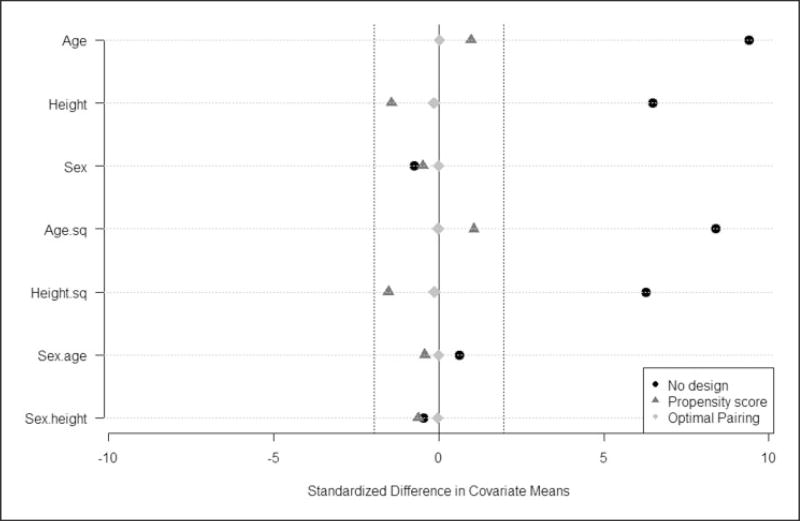
Many methods have been proposed to assess balance in covariates (some reviewed by Imbens and Rubin⁸). We also calculated the standardized mean differences between the exposed and unexposed children (before and after matching on age, height, and sex using propensity score calipers and optimal pairing) of the variables age, age², height, height², sex, sex×age, and sex×height. Figure 4 shows that the standardized mean differences between exposed and non-exposed children were reduced after propensity score matching for all variables included when estimating the propensity score (i.e. age, height, and sex), as well as for the variables not included in the propensity score (i.e. age², height², sex×age, and sex×height) because these were correlated with the estimated propensity score. Note that smaller calipers could have been chosen but minimal improvement was achieved with respect to overall covariate balance. The “Love” plot³⁶ also suggests excellent balance achieved by the optimal matching strategy between the exposed and unexposed children.

Figure 4.

Standardized mean differences for the variables age, height, sex, age², height², sex × age, and sex × height for the non-exposed vs. exposed children before matching (black dots), after propensity score matching (d) (darker grey triangles), and after optimal pair matching (e) (lighter grey diamonds) (“Love” plots).

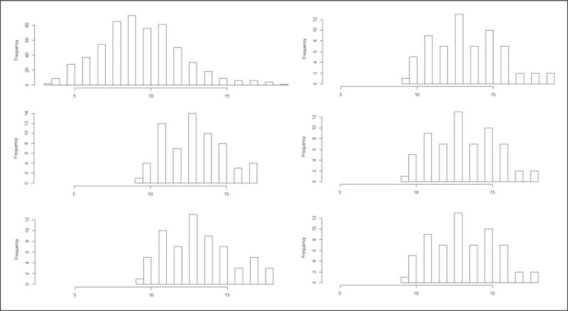
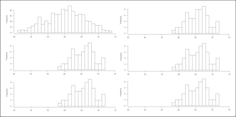
Another way of assessing balance for continuous covariates, which can provide more detailed insights than the standard “Love” plots presented in Figure 4, is to present the empirical distributions of age and height for the exposed vs. non-exposed children before and after matching (Figures 5 and 6). For conciseness, we presented these distributions of the continuous variables age and height among the exposed and unexposed children before and after matching on age, height, and sex only for experiments 4 and 5 (i.e. for the propensity score caliper (d) and optimal pairing (e) approaches). As shown in Figures 5 and 6, the balance has improved for the variables age and height after propensity score matching and after optimal pair matching.

Figure 5.

Empirical distributions of the variables age among non-exposed (left panels) and exposed (right panels) children in the original dataset (a) (top panels), after propensity score matching (d) (middle panels), and after optimal pair matching (e) (bottom panels) [Kolmogorov–Smirnov ’distances’ for: (1) the difference in age distributions of the non-exposed vs. exposed children in the original dataset (a) = 0.56, (2) the difference in age distributions of the non-exposed vs. exposed children after propensity score matching (d) = 0.10, (3) the difference in age distributions of the non-exposed vs. exposed children after optimal pair matching (e) = 0.06].

Figure 6.

Empirical distributions of the variables height among non-exposed (left panels) and exposed (right panels) children in the original dataset (a) (top panels), after propensity score matching (d) (middle panels), and after optimal pair matching (e) (bottom panels) [Kolmogorov–Smirnov ’distances’ for: (1) the difference in height distributions of the non-exposed vs. exposed children in the original dataset (a) = 0.47, (2) the difference in height distributions of the non-exposed vs. exposed children after propensity score matching (d) = 0.16, (3) the difference in height distributions of the non-exposed vs. exposed children after optimal pair matching (e) = 0.05].

We also reported Kolmogorov–Smirnov (KS) “distances” between the univariate distributions of the continuous background variables age and height for the exposed children and those distributions for the unexposed children (before and after matching using propensity score caliper (d) and optimal pairing (e))

$${\text{KS}}_{\text{no design}}={\text{sup}}_{\mathrm{x}\mathrm{\epsilon }\{\text{no design}\}}\Vert {\mathrm{F}}_{\text{Smoking}}(\mathrm{x})-{\mathrm{F}}_{\text{Non}-\text{smoking}}(\mathrm{x})\Vert$$

$${\text{KS}}_{\text{propensity score}}={\text{sup}}_{\mathrm{x}\mathrm{\epsilon }\{\text{propensity score}\}}\Vert {\mathrm{F}}_{\text{Smoking}}(\mathrm{x})-{\mathrm{F}}_{\text{Non}-\text{smoking}}(\mathrm{x})\Vert$$

$${\text{KS}}_{\text{optimal pairing}}={\text{sup}}_{\mathrm{x}\mathrm{\epsilon }\{\text{optimal pairing}\}}\Vert {\mathrm{F}}_{\text{Smoking}}(\mathrm{x})-{\mathrm{F}}_{\text{Non}-\text{smoking}}(\mathrm{x})\Vert$$

The KS “distances” reflect how much the univariate distributions of the variables for the exposed children differ from those distributions for the unexposed children (see Figures 5 and 6).

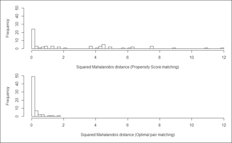
The distributions of the squared Mahalanobis distances between propensity score (top panel) vs. optimal pairs (bottom panel) are presented in Figure 7. Although the range of pairwise squared Mahalanobis distances is between 0 and 12 for the propensity score matched pairs, with the optimal pair matching approach, the range of these squared distances is between 0 and 2, which suggests better pair matching.

Figure 7.

Distribution of the squared Mahalanobis distances between propensity score (d) and optimal (e) matched pairs.

3.2.6 Analysis phase (third stage): various standard regression-based outcome analysis-phase strategies at the super-population level

(i) T-test/crude regression analysis (i.e. no covariate adjustment)

An initial t-test can be conducted comparing the mean FEV-1 among children with smoking parents to the mean FEV-1 among children with non-smoking parents. This is equivalent, assuming that the treatment effect is constant and additive for all units and that the residual variances in both groups are the same, to regressing the dependent variable, FEV-1, on the indicator for exposure of interest “parental smoking,” and examining the size and statistical significance of the coefficient of the indicator.

(ii) Standard linear regression model with simple linear adjustment

The second analysis regresses the dependent variable FEV-1 on the exposure of interest “parental smoking” as in analysis (i) but also linearly “adjusts” for the three covariates available in the dataset, i.e. age, height, and sex, by including them in the regression model, and making the analogous assumptions as with the first analysis. The distributions of the outcome of interest FEV-1 across children with parents who smoke and not, stratified by sex, are presented in the Supplementary Figure 1. We also assessed the significance of interaction terms between parental smoking and the three covariates, and found limited evidence of interactions (p_interaction = 0.14 for smoking×age, p_interaction = 0.10 for smoking×height, and p_interaction = 0.26 for smoking×sex). We also found little evidence against the linearity assumption of the associations between (1) age and FEV-1, and (2) height and FEV-1 (see Supplementary Figure 2). Other versions of this regression were investigated in the original dataset, that is, using all 654 units (i.e. omitting conceptual and design stages).²³

3.2.7 Analysis-phase strategies (third stage) at the finite-population level

(i) Analysis using Fisherian (Fiducial) inference in the finite population

Because there were three plausible hypothetical randomized experiments, we perform randomization-based tests assuming the data arise from: (i) the complete randomization experiment (D.1), (ii) the rerandomized experiment (D.2), and (iii) the pairwise randomized experiment (E). That is, we test the Fisher null hypothesis of no effect of parental smoking on children’s FEV-1 in the finite population sample by performing a stochastic proof by contradiction. We first assume the null hypothesis of absolutely no effect of treatment versus control, so that we know all potential outcomes and thus know what the value of any test statistic would be obtained under any treatment assignment. Then, for the completely randomized experiment (D.1), we permuted the treatment assignment among the 126 children such that half of them get exposed and obtain 126-choose-23 different treatment assignments. Similarly, for the hypothetical rerandomized experiment (D.2), we rerandomized the 126 children such that half of them get exposed but the two groups have similar background covariates’ means. Finally, for the paired randomized experiment, we choose one member of each of the 63 pairs to be considered treated, and thereby obtain 2⁶³ different treatment assignments. We conducted 10,000 random draws of permuted (1) completely randomized (D.1), (2) rerandomized (D.2), and (3) pair randomized treatment assignments (E), and calculate the following statistic in each permuted allocation:

1. T_{t-completely randomized D.1} = t-test statistic comparing the mean FEV-1 among exposed and unexposed children (different group variances),

2. T_{t-rerandomized D.2} = t-statistic of the regression coefficient of smoking when regressing FEV-1 on smoking, age, height, and sex, and

3. T_{t-paired randomized E} = paired t-test statistic comparing the means FEV-1 among exposed vs. unexposed children.

We obtain Fiducial intervals by inverting the sharp null hypothesis tests for different constant additive effects, as described in Imbens and Rubin.⁸

(ii) Analysis using Bayesian inference to estimate the posterior distribution of the average causal effect (ACE) and its 95% probability interval in the finite population

We now consider the Bayesian approach initially proposed by Rubin³⁷ and described in Imbens and Rubin.⁸ Briefly, we first specify distributions for the potential outcomes conditional on covariates, here for simplicity independent and identically distributed normal ones. Because we consider only the plausible hypothetical randomized experiments (D.1, D.2, and E) in this section, we assume ignorable exposure assignment (i.e. P(Smoking_i=1 | FEV-1_i^obs, FEV-1_i^mis, Age_i^obs, Height_i^obs, Sex_i^obs) = P(Smoking_i=1 | FEV-1_i^obs, Age_i^obs, Height_i^obs, Sex_i^obs), where FEV-1_i^obs and FEV-1_i^mis represent the observed and missing FEV-1 potential outcomes for the i^th unit).³⁷ We impute the missing potential outcomes among the exposed and non-exposed groups separately, allowing for different normal models (conditional on the intercept and the three covariates available in the dataset, i.e. age, height, and sex), that is, different means (µ_i,Smoking = β_Smoking X_i and µ_{i,Non-smoking} = β_Non-smoking X_i, where X_i represents the constant, age_i, height_i, and sex_i) and different variances in the exposure groups (σ_Smoking² and σ_Non-smoking²). The goal is to draw multiple values of FEV-1_i^mis conditional on FEV-1_i^obs, Smoking_i^obs, Age_i^obs, Height_i^obs, Sex_i^obs, and the parameters β_Smoking, β_Non-Smoking, σ_Smoking², σ_Non-smoking². To accomplish this, we need to calculate the posterior distribution for the parameters. We assume flat priors for the parameters β and σ², that is

$$\mathrm{p}({\beta }_{\text{Smoking}},{\sigma }_{\text{Smoking}}^2)\infty {\sigma }_{\text{Smoking}}^{-2}\text{ and }\mathrm{p}({\beta }_{\text{Non}-\text{smoking}},{\sigma }_{\text{Non}-\text{smoking}}^2)\infty {\sigma }_{\text{Non}-\text{smoking}}^{-2}$$

We use two separate Gibbs samplers to impute: (1) the missing control potential outcomes among the treated, and (2) the missing treated potential outcomes among the controls, reflecting independent prior distributions for these parameters.

For instance, to impute the control missing potential outcomes, i.e. FEV_i-1^mis=FEV_i-1[Smoking_i=0)] among the exposed children

1. we draw σ_Non-smoking² such that:

   1/σ_Non-smoking² ~ {1/ [(n_Non-Smoking − 4) s_Non-Smoking²]} χ² with n_Non-Smoking − 4 degrees of freedom, where n_Non-Smoking, s_Non-Smoking² are the number of children with non-smoking parents and the FEV-1 sample variance among the children with non-smoking parents, respectively;

2. we then draw β_Non-Smoking conditional on σ_Non-smoking², FEV_i-1^obs, Smoking_i^obs, X_i^obs from a normal distribution with mean equal to [(X_Non-Smoking^T X_Non-Smoking)⁻¹ X_Non-Smoking^T FEV_i-1_Non-Smoking] and variance-covariance matrix [X_Non-Smoking^T X_Non-Smoking)⁻¹ σ_Non-smoking²], and finally,

3. we draw the missing control potential outcomes among the treated; that is, for unit i such Smoking_i=1, we draw FEV-1_i^mis conditional on FEV-1_i^obs, W_i, β_Non-Smoking, and σ_Non-smoking² independently from a normal distribution with mean [X_i^obs β_Non-Smoking] and variance σ_Non-smoking².

At each replication, we impute the missing potential outcomes in both groups and calculate the average causal effect (ACE), i.e. the mean difference in FEV-1 among all children when having smoking parents vs. when having non-smoking parents. We repeat this procedure 10,000 times and thereby obtain 10,000 draws from the posterior distribution of the ACE.

(iii) Combining the Bayesian and Fisherian approaches

The Bayesian approach relies on the model specification to be approximately correct, whereas the Fisherian procedure provides a non-parametric procedure to test the sharp null hypothesis. We propose to use a different, and possibly more interesting, statistic than T_{t-completely randomized D.1}, T_{t-rerandomized D.2}, and T_{t-paired randomized E} calculated from the approximated Bayesian posterior distribution of the average causal effect to test the sharp null hypothesis, T_t-Bayesian = | posterior mean of the ACE | / standard deviation of the ACE. The idea to use a statistic based on a model for the Fisher test goes back at least to Brillinger et al.³⁸

3.3 Results from our example

3.3.1 Estimated average causal effects (ACE) and associated asymptotic 95% confidence intervals in the super-population (see Table 3)

Table 3.

Analysis stage: comparison of the average causal effect (ACE) estimates and intervals across methods.

Hypothetical experiment/Design stage methods	Analysis method	Number of units	Estimate of the ACE	95% Confidence interval
Hypothetical experiment (A) / No design (a)	Crude comparison	654	0.71	[0.50; 0.93]
	Standard linear regression with no interactions	654	−0.09	[−0.20; 0.03]
Hypothetical experiment (B) / Trimming (b) (Restriction to girls between 10 and 18 years old and height between 60 and 69 inches and to boys between 9 and 18 years and height between 58 to 72 inches)	Crude comparison	361	0.18	[−0.03; 0.39]
	Standard linear regression with no interactions	361	−0.16	[−0.30; −0.03]
Hypothetical experiment (C) / Stratified matching (c) (cem R package)	Crude comparison	273	−0.16	[−0.37; 0.05]
	Standard linear regression with no interactions	273	−0.16	[−0.30; −0.03]
Hypothetical experiments (D.1 and D.2) / Propensity score matching (d) (caliper=1 standard deviation of the propensity score, Matching R package)	Crude comparison	126	−0.20	[−0.43; 0.03]
	Standard linear regression with no interactions	126	−0.23	[−0.46; −0.00]
Hypothetical experiment (E) / Optimal pair matching (e) (Mimimum squared Mahalanobis distance, optmatch R package)	Crude comparison	126	−0.19	[−0.46; 0.08]
	Standard linear regression with no interactions	126	−0.18	[−0.35; −0.01]

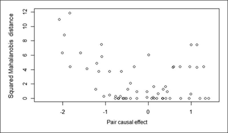
The first two rows of Table 3 summarize the two analyses with no design stage, and both indicate a beneficial or uncertain effect of smoking parents on children’s FEV-1. From Table 3, the trimming approach provides estimated ACEs that indicate essentially slightly beneficial or uncertain effects of parental smoking on children’s FEV-1. From the fifth and sixth rows of Table 3, we see that, with the stratified matching strategy, the estimated ACEs indicate some possible negative effects of parental smoking on children’s FEV-1. With 126 units, but restricting the data to pairs of children who are “similar” with respect to age, height, and sex, the propensity matched sampling approach estimates the crude and adjusted estimated effects of parental smoking on children’s FEV-1 to be negative. That is, the mean FEV-1 among children with parents who smoke was estimated to be lower than the mean FEV-1 among children with non-smoking parents. The squared Mahalanobis distances between propensity score matched pairs are greater for the negative estimated paired causal effects as shown in Figure 8, suggesting some “outlying” pairs. If we removed a few pairs with squared Mahalanobis distances between propensity score pairs greater than 8, 6, 4, or 2 (i.e. resulting in 60, 54, 42, and 38 pairs, respectively), the estimated crude ACEs change from −0.20 to −0.14, −0.11, −0.07, and 0.01, respectively. With 63 “optimal” pairs, the crude and adjusted estimated effects of parental smoking on children’s FEV-1 also suggest negative effects.

Figure 8.

Pairwise squared Mahalanobis distances between propensity score matched pairs (d) versus the estimated paired causal effects (d).

3.3.2 Fisherian and Bayesian inferences in the finite population

(i) Fisherian (Fiducial) inference in the finite population

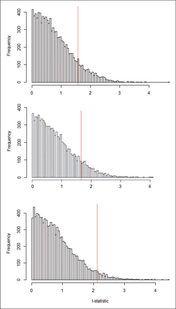
The approximated null randomization distributions of the chosen statistics T_{t-completely randomized D.1}, T_{t-rerandomized D.2}, and T_{t-paired randomized E} (based on 10,000 draws of the permuted treatment assignment) are presented in Figure 9. The proportion of the equiprobable treatment allocations under randomized assignment that led to values of the statistics, T_{t-completely randomized D.1}, T_{t-rerandomized D.2}, and T_{t-paired randomized E}, as large or larger than the observed statistic T^obs_{t-completely randomized D.1} = 1.57, T^obs_{t-rerandomized D.2} = 1.66, and T^obs_{t-paired randomized E} = 2.12 were equal to p-value_{completely randomized D.1} = 0.12, p-value_{rerandomized D.2} = 0.10, and p-value_{paired randomized E} = 0.04, respectively, all suggesting significant effects of parental smoking.

Figure 9.

Approximate null randomization distributions of t-statistics under the reconstructed randomized experiments (T_{t-completely randomized D.1}, T_{t-rerandomized D.2}, and T_{t-paired-randomized E}) and observed t-statistics (T^obs_{t-completely randomized D.1}, T^obs_{t-rerandomized D.2}, and T^obs_{t-paired-randomized E}) [Randomization-based p-value_{completely randomized D.1} = 0.12, T^obs_{t-completely randomized D.1} = 1.57, and 95% Fiducial interval _{completely randomized D.1} = −0.52 to 0.06, Randomization-based p-value_{rerandomized D.2} = 0.10, T^obs_{t-rerandomized D.2} = 1.66, and 95% Fiducial interval_{rerandomized D.2} = −0.33 to 0.03, and Randomization-based p-value_{paired randomized E} = 0.04, T^obs_{t-paired-randomized E} = 2.12, and 95% Fiducial interval_{paired randomized E} = −0.37 to −0.02].

Inverting these sharp null hypothesis tests for different values of average causal effects across the three reconstructed randomized experiments led to 95% Fiducial intervals equal to [−0.52 to 0.06]_{completely randomized D.1}, [−0.33 to 0.03]_{rerandomized D.2}, and [−0.37 to −0.02]_{paired randomized E}, again suggesting negative effects of parental smoking on children’s FEV-1.

(ii) Bayesian inference for the posterior distribution of the average causal effect (ACE) and its 95% probability interval in the finite population

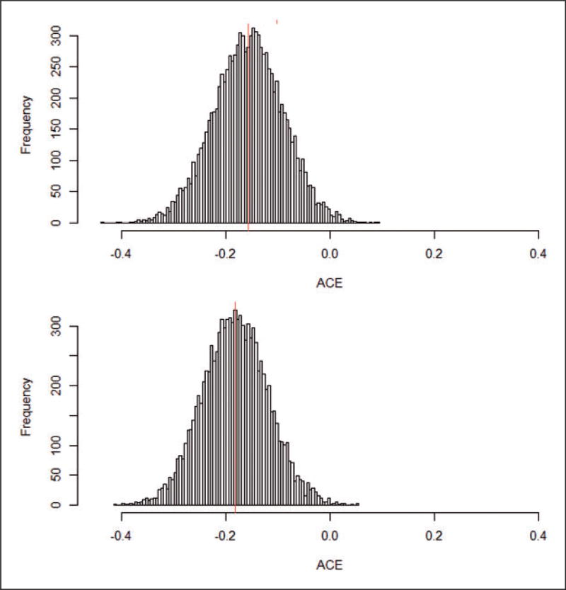
The posterior distributions of the average causal effect (ACE) using the matched-sampling datasets obtained via the propensity score (top panel) and the optimal pair matching (bottom panel) approaches are presented in Figure 10. The posterior means are −0.16 and −0.18 and the 95% probability intervals are [−0.29 to −0.04] and [−0.30 to −0.06], respectively, suggesting fairly clear evidence of negative effects of parental smoking on children’s FEV-1.

Figure 10.

Estimated distributions and posterior means of the average causal effect (ACE) in the propensity score matched (d) [mean: −0.16 and 95% posterior interval: −0.29; −0.03] and optimal paired (e) [mean: −0.18 and 95% posterior interval: −0.30; −0.06] data sets.

(iii) Combining the Bayesian and Fisherian approaches

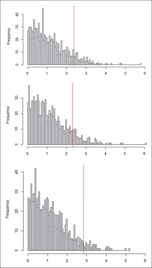
The approximated null randomization distributions of the chosen statistics T_{t-completely randomized D.1 and Bayesian}, T_{t-rerandomized D.2 and Bayesian}, and T_{t-paired randomized E and Bayesian}, respectively (based on 10,000 draws of the permuted treatment assignment) are presented in Figure 11. The proportion of the equiprobable treatment allocations under randomized assignment that led to statistics T_{t-completely randomized D.1 and Bayesian}, T_{t-rerandomized D.2 and Bayesian}, and T_{t-paired randomized E and Bayesian} with as large or larger values than the observed statistic T^obs_{t-completely randomized D.1 and Bayesian} = 2.39, T^obs_{t-rerandomized D.2 and Bayesian} = 2.31, and T^obs_{t-paired randomized E and Bayesian} = 2.84 were equal to p-value_{completely randomized D.1 and Bayesian} = 0.09, p-value_{rerandomized D.2 and Bayesian} = 0.10, and p-value_{paired randomized E and Bayesian} = 0.04, respectively, again suggesting that parental smoking is not good for children’s FEV-1.

Figure 11.

Approximate null randomization distributions of t-statistics under the reconstructed randomized experiments (Tt-completely randomized D.1 and Bayesian, Tt-rerandomized D.2 and Bayesian, and Tt-paired-randomized E and Bayesian) and observed tstatistics (Tobs t-completely randomized D.1 and Bayesian, Tobs t-rerandomized D.2 and Bayesian, and Tobs t-paired-randomized E and Bayesian) [Randomization-based p-valuecompletely randomized D.1 and Bayesian = 0.09, Tobs t-completely randomized D.1 and Bayesian = 2.39, Randomization-based p-valuererandomized D.2 = 0.10, Tobs t-rerandomized D.2 = 2.31, Randomization-based p-valuepaired randomized E = 0.04, and Tobs t-paired-randomized E = 2.84].

4 Discussion

Even though our approach uses fewer units in the analysis phase (i.e. third stage) compared to the standard model-based approach without conceptual or design phases, it can still reach relevant conclusions, arguably more credible than the standard ones. Our results contrast with the naive idea that more units of analysis always bring more statistical power to detect causal effects. Our final causal conclusion appears to not fully support the reported associational estimate in the Harvard Six Cities longitudinal study.³⁹ In this well-known study, Wang et al. reported that each pack per day smoked by the mother was not associated with a significant reduction in FEV-1 among children 6–10 years old (Point estimate on the multiplicative scale: 0.4% and associated 95%CI: [−0.9% to 0.1%] after “adjusting/controlling” for age, height, city of residence, and parental education).

Once causality is suspected, the next step is to acquire medical knowledge, for instance, trying to understand biological mechanisms explaining why exposure to parental smoking causes reduced lung function (e.g. via smoking-specific inflammatory biomarkers). Also, interventions that may curtail smoking can be explored, for instance by trying to predict the occurrence of smoking among parents using the background covariates to predict smoking.

Our approach with conceptual and design phases facilitates an approximation to the ideal conditions of a randomized experiment and has the tremendous advantages that these phases can be conducted blind to the outcome data and that their formulation relies on creative thinking by the environmental epidemiologist. Obviously, inferences are restricted to children who remain in the sample. Our inferential statements apply to the studied finite subsample. However, the causal question of interest related to a larger but still finite population. Extrapolation to children with covariate values beyond values observed in the matching children should generally be done with great caution because the data do not provide direct information for treated children without control matches. This is one advantage of classical randomization-based inference advocated here vs. the more common purely model-based approaches using the entire data set. Fisher randomization-based p-values associated with explicit designs can be easily conceptualized and obtained, and no asymptotic distributional assumptions are used. In our approach, as in the design of randomized experiments, we eschew the use of outcome variables to create the matched pairs.⁴⁰ Instead, we attempt to recreate hypothetical completely randomized, rerandomized, and matched pair randomized experiments. This process was implied more than a half century ago by Dorn’s 1952 sage advice, repeated by Cochran,⁴¹ “How would the study be conducted if it were possible to do it by controlled experimentation?”.

A causal investigation needs to examine the implicit assumption that the hypothetical set of control children is effectively stochastically identical to the set of exposed children on all their observed background variables. This assumption is explicit, transparent, and readily assessed by simple visual diagnostics. For instance, Figure 4 shows the effect of matching on the standardized mean differences between exposed and non-exposed children for the covariates age, height, and sex (allowing for linear and quadratic relationships, as well as interactions). If all covariates and their nonlinear terms were as well matched, then a logical, although tentative, conclusion can be reached concerning the evidence that parental smoking was the cause of any discrepancies between the exposed and non-exposed children in lung function, in the sense that if we could eliminate parental smoking without any untoward consequences of the intervention, this difference in lung function would be found for experimental data. Figures 3 and 4 present the effect of matching (via propensity score and optimal pairing) on the distributions of the continuous covariates age and height, respectively, i.e. in this case, matching created almost identical age and height distributions for exposed and non-exposed children, which is ideal for eliminating any confounding arising from age and height.

We considered different methods using either stratification, propensity score intersection (caliper) matching, or optimal pairing using Mahalanobis distance. In our data set, the optimal pairing led to very well-matched children and appears to be ideal for our data as a design stage procedure preceding the (multiple) imputation of the missing potential outcomes. In settings with more than three background covariates, minimizing the squared Mahalanobis distance will not be as satisfactory as in settings with low-dimension covariates because every unit is likely to be far apart on this full-rank metric,²¹ so it may be better to minimize this distance within pairs in the same propensity score caliper only with respect to the continuous covariates (e.g. using the procedure proposed in Rosenbaum and Rubin²⁵). Other balancing criteria could be used that may be more relevant to optimize than some function involving Mahalanobis distance. This optimized criterion-based rejection, which we call the OCBR approach, which discards units that do not satisfy the criterion may be attractive and flexible with respect to the choice of a criterion because it can combine several criteria measuring covariates’ balance. If the a priori optimization criteria would have combined diagnostics of covariates imbalance, such as 1) differences in covariates means and variances between exposed and unexposed, followed by, 2) Kolmogorov–Smirnov distances between continuous covariates distributions in the exposed vs. unexposed, these balancing diagnostics would automatically be satisfied by the procedure.

Some drawbacks of the OCBR strategy are that the approach is computationally intensive and currently lacks software implementation for even simple criterion and is entirely unexplored for even more exotic and creative criterion. The optimal matching strategy also selects only one matched dataset, the one with minimum total squared Mahalanobis distance, which may restrict pure randomization-based inference. Future work should consider criterion-based rejection (CBR) approaches constructing matched datasets satisfying a balancing criterion instead of an optimization function.

Unmatched data from exposed children that have background characteristics that differ markedly from the background characteristics of unexposed children are discarded in our approach; yet such children values are automatically included in standard model-based regression, and their inclusion can distort the prediction of missing potential outcomes and therefore the causal conclusion. The selection of matched subgroups is with purpose and can be interpreted as a distillation of the sample to the units most relevant for the causal analysis of interest. Also, even if the point and interval estimates were to agree numerically between our analysis and a standard analysis, the “results and associated conclusions” are not necessarily the same. Not only are our conclusions explicitly limited to children represented by groups or pairs that are well matched, but the assumptions underlying the hypothetical randomized experiments are entirely transparent and accessible, as exemplified by Figures 4 to 8 and Table 2, and therefore facilitate discussions among scientists about their veracity.

We feel that our matched-sampling strategy, based on the hypothetical randomization that created the sets of exposed versus non-exposed units, followed by the analysis of data by randomization tests, relies on powerful and modern computing to implement both (a) the creation and analysis of exchangeable groups or pairs, and (b) the fiducial tests themselves. Of particular interest, these types of analyses using (1) matched-sampling techniques, (2) constructing a t-statistic summarizing the Bayesian analysis, and (3) performing non-parametric Fisherian inference, have apparently not been previously done, or even contemplated, in environmental epidemiology. Combining the Bayesian and Fisherian inference frameworks could lead better statistical properties.⁴²

Our approach has the potential to have a broad impact on many biomedical fields, especially environmental epidemiology, because extensions implicitly propose a universal framework using classical ideas from randomized experiments to tackle causal questions examining the joint health effects of multi-factorial environmental exposures (e.g. mixtures of indoor and outdoor air pollutants, weather conditions, physical activity, etc.). Here, when facing such questions, we propose embedding an observational data set within the context of a hypothetical multi-factorial randomized experiment. It is important to emphasize that this proposed approach is not restricted to relatively simple settings, but it generalizes to situations involving complex data structures (e.g. longitudinal data; “mediators” – to examine putative causal pathways; and high-dimensional data – to help discover the etiology of complex diseases or disorders).

5 Conclusions

Causal analyses should demonstrate to the readers that it is plausible to assume that the estimated causal effect would be of similar magnitude to those that would be obtained had the researcher conducted a real randomized experiment with the same random treatment assignment assumed in the experiment. We propose a logically and practically transparent, yet mathematically precise and rigorous, approach to study the health effects of multi-factorial exposures, including the environmental “exposome” resulting in causal inferences that are valid under explicitly stated assumptions. We illustrated our method using a simple dataset with three background covariates. However, this four-stage approach can be used with a larger number of covariates. This framework can also be used to study biological mechanisms and susceptibility to complex diseases resulting from the joint effects of multiple factors. Because of its conceptual links to hypothetical interventions, it can suggest policies for reducing environmental pollutants and thereby preventing diseases. Finally, because of its logical transparency, it should promote education across, and communication between, researchers and policy-makers.

References

- 1.Dockery DW, Pope CA, 3rd, Xu X, et al. An association between air pollution and mortality in six U.S. cities. N Engl J Med. 1993;329:1753–1759. doi: 10.1056/NEJM199312093292401. [DOI] [PubMed] [Google Scholar]
- 2.Bell ML, Peng RD, Dominici F. The exposure-response curve for ozone and risk of mortality and the adequacy of current ozone regulations. Environ Health Perspect. 2006;114:532–536. doi: 10.1289/ehp.8816. [DOI] [PMC free article] [PubMed] [Google Scholar]
- 3.Schwartz J. Air pollution and blood markers of cardiovascular risk. Environ Health Perspect. 2001;109:405–409. doi: 10.1289/ehp.01109s3405. [DOI] [PMC free article] [PubMed] [Google Scholar]
- 4.Corbo GM, Agabiti N, Pistelli R, et al. Parental smoking and lung function: misclassification due to background exposure to passive smoking. Respir Med. 2007;101:768–773. doi: 10.1016/j.rmed.2006.08.004. [DOI] [PubMed] [Google Scholar]
- 5.Holland P. Statistics and causal inference (with discussion) J Am Stat Assoc. 1986;81:945–970. [Google Scholar]
- 6.Angrist JD, Imbens GW, Rubin DB. Identification of causal effects using instrumental variables (with discussion) J Am Stat Assoc. 1996;91:444–472. [Google Scholar]
- 7.Imbens G, Rubin DB. Rubin causal model. In: Durlauf SM, Blume CE, editors. The New Palgrave Dictionary of Economics. 2. Vol. 7. New York: Palgrave McMillan; 2008. pp. 255–262. [Google Scholar]
- 8.Imbens G, Rubin DB. Causal inference for statistics, social, and biomedical sciences: an introduction. New York, NY: Cambridge University Press; 2015. [Google Scholar]
- 9.Rubin DB. Comment: Neyman (1923) and causal inference in experiments and observational studies. Stat Sci. 1990;5:472. [Google Scholar]
- 10.Rubin DB. Estimating causal effects of treatments in randomized and nonrandomized studies. J Educ Psychol. 1974;66:688. [Google Scholar]
- 11.Pearl J. Causal diagrams for empirical research. Biometrika. 1995;82:669–688. [Google Scholar]
- 12.Rubin DB. The design versus the analysis of observational studies for causal effects: parallels with the design of randomized trials. Stat Med. 2007;26:20. doi: 10.1002/sim.2739. [DOI] [PubMed] [Google Scholar]
- 13.Rubin DB. For objective causal inference, design trumps analysis. Ann Appl Stat. 2008;2:808. [Google Scholar]
- 14.Fisher RA. Statistical methods for research workers. 1. Edinburgh: Oliver and Boyd; 1925. [Google Scholar]
- 15.Fisher RA. Design of experiments. Edinburgh: Oliver and Boyd; 1935. [Google Scholar]
- 16.Kempthorne O. The design and analysis of experiments. Robert Krieger Publishing Company; 1952. [Google Scholar]
- 17.Cochran WG, Cox G. Experimental design. Wiley Classics Library; 1957. [Google Scholar]
- 18.Cochran WG. The effectiveness of adjustment by subclassification in removing bias in observational studies. Biometrics. 1968;24:295–314. [PubMed] [Google Scholar]
- 19.Cochran WG, Rubin DB. Controlling bias in observational studies: a review. Sankhya: Ind J Stat. 1973;35:417–446. [Google Scholar]
- 20.Rubin DB. The use of matched sampling and regression adjustment to remove bias in observational studies. Biometrics. 1973;29:184–203. [Google Scholar]
- 21.Rubin DB. Matched sampling for causal effects. New York, NY: Cambridge University Press; 2006. p. 489. [Google Scholar]
- 22.Tager IB, Weiss ST, Rosner B, et al. Effect of parental cigarette smoking on the pulmonary function of children. Am J Epidemiol. 1979;110:15–26. doi: 10.1093/oxfordjournals.aje.a112783. [DOI] [PubMed] [Google Scholar]
- 23.Kahn M. An exhalent problem for teaching statistics. J Stat Educ. 2005;13 [Google Scholar]
- 24.Box GEP, Hunter JS, Hunter WG, et al. Statistics for experimenters: an introduction to design, data analysis, and model building. New York: Wiley; 1978. p. 653. [Google Scholar]
- 25.Rosenbaum P, Rubin DB. Constructing a control group using multivariate matched sampling incorporating the propensity score. Am Stat. 1985;39:33–38. [Google Scholar]
- 26.Sekhon J. Multivariate and propensity score matching software with automated balance optimization: the matching package for R. J Stat Software. 2011;42 [Google Scholar]
- 27.Hansen BB, Olsen Klopfer S. Optimal full matching and related designs via network flows. J Computat Graph Stat. 2006;15:609–627. [Google Scholar]
- 28.Carles S, Charles MA, Heude B, et al. Joint Bayesian weight and height postnatal growth model to study the effects of maternal smoking during pregnancy. Stat Med. 2017;36:3990–4006. doi: 10.1002/sim.7407. [DOI] [PubMed] [Google Scholar]
- 29.Rubin DB. Using multivariate matched sampling and regression adjustment to control bias in observational studies. J Am Stat Assoc. 1979;74:318–328. [Google Scholar]
- 30.Gutman R, Rubin DB. Robust estimation of causal effects of binary treatments in unconfounded studies with dichotomous outcomes. Stat Med. 2013;32:1795–1814. doi: 10.1002/sim.5627. [DOI] [PubMed] [Google Scholar]
- 31.Rubin DB. Multivariate matching methods that are equal percent bias reducing, I: Some examples. Biometrics. 1976;32:109–120. [Google Scholar]
- 32.Andridge RR, Little RJ. A review of hot deck imputation for survey non-response. Int Stat Rev. 2010;78:40–64. doi: 10.1111/j.1751-5823.2010.00103.x. [DOI] [PMC free article] [PubMed] [Google Scholar]
- 33.Iacus SM, King G, Porro G. Causal inference without balance checking: coarsened exact matching. Political analysis. 2011:mpr013. [Google Scholar]
- 34.Althauser R, Rubin DB. The computerized construction of a matched sample. Am J Sociol. 1970;76:325–346. [Google Scholar]
- 35.Morgan K, Rubin DB. Rerandomization to improve covariate balance in experiments. Ann Stat. 2012;40:1263–1282. [Google Scholar]
- 36.Ahmed A, Husain A, Love TE, et al. Heart failure, chronic diuretic use, and increase in mortality and hospitalization: an observational study using propensity score methods. Eur Heart J. 2006;27:1431–1439. doi: 10.1093/eurheartj/ehi890. [DOI] [PMC free article] [PubMed] [Google Scholar]
- 37.Rubin DB. Bayesian inference for causal effects: the role of randomization. Ann Stat. 1978;6:34–58. [Google Scholar]
- 38.Brillinger DR, Jones LV, Tukey JW. Report of the Statistical Task Force to the Weather Modification Advisory Board. Anonymous The management of weather resources, Volume II. 1978:25, F-5. [Google Scholar]
- 39.Wang X, Wypij D, Gold DR, et al. A longitudinal study of the effects of parental smoking on pulmonary function in children 6–18 years. Am J Respir Crit Care Med. 1994;149:1420–1425. doi: 10.1164/ajrccm.149.6.8004293. [DOI] [PubMed] [Google Scholar]
- 40.Rubin DB. “Author’s reply” to letter by I. Shrier re: The design versus the analysis of observational studies for causal effects: parallels with the design of randomized trials (2007) Stat Med. 2008;27:2741–2742. doi: 10.1002/sim.3172. [DOI] [PubMed] [Google Scholar]
- 41.Cochran WG, Moses LE, Mosteller F. Planning and analysis of observational studies. New York, NY: Wiley; 1983. p. 145. [Google Scholar]
- 42.Rubin DB. More powerful randomization-based p-values in double-blind trials with non-compliance. Stat Med. 1998;17:371–385. doi: 10.1002/(sici)1097-0258(19980215)17:3<371::aid-sim768>3.0.co;2-o. [DOI] [PubMed] [Google Scholar]
Associated Data
This section collects any data citations, data availability statements, or supplementary materials included in this article.