Influence of the size and curvedness of neural projections on the orientationally averaged diffusion MR signal

Abstract

Neuronal and glial projections can be envisioned to be tubes of infinitesimal diameter as far as diffusion magnetic resonance (MR) measurements via clinical scanners are concerned. Recent experimental studies indicate that the decay of the orientationally-averaged signal in white-matter may be characterized by the power-law, Ē(q) ∝ q⁻¹, where q is the wavenumber determined by the parameters of the pulsed field gradient measurements. One particular study by McKinnon et al. [1] reports a distinctively faster decay in gray-matter. Here, we assess the role of the size and curvature of the neurites and glial arborizations in these experimental findings. To this end, we studied the signal decay for diffusion along general curves at all three temporal regimes of the traditional pulsed field gradient measurements. We show that for curvy projections, employment of longer pulse durations leads to a disappearance of the q⁻¹ decay, while such decay is robust when narrow gradient pulses are used. Thus, in clinical acquisitions, the lack of such a decay for a fibrous specimen can be seen as indicative of fibers that are curved. We note that the above discussion is valid for an intermediate range of q-values as the true asymptotic behavior of the signal decay is Ē(q) ∝ q⁻⁴ for narrow pulses (through Debye-Porod law) or steeper for longer pulses. This study is expected to provide insights for interpreting the diffusion-weighted images of the central nervous system and aid in the design of acquisition strategies.

1 INTRODUCTION

Diffusion-sensitized magnetic resonance acquisitions have been employed to recover the microscopic building blocks of complex nervous tissue. Simplified models exploiting the compartmentalized structure of the tissue are instrumental in this endeavor. Water molecules in the intra- and extra-cellular spaces have been envisioned to form separate compartments with different signal characteristics [2]. The intracellular signal is also thought to represent the superposition of contributions from cells of different types, shapes, and orientations [3]. The same argument has been employed even for a single neuron wherein each neurite has been considered to comprise a collection of straight compartments [4]. Such representation of neurites as slender cylinders distributed in random orientations within the voxel is perhaps the model most relevant to the current study.

The diameter of neurites, and in fact all neural projections, is so small that diffusion in the transverse plane may be negligible. More explicitly, a cylinder with the same diameter as a neurite would not suffer any signal loss in a typical clinical diffusion MRI measurement when the diffusion gradients are applied in the direction perpendicular to the cylinder’s axis. This justifies assigning zero value to transverse diffusivity for molecules confined in the cylinder. Such behavior [5] was indeed observed for N-acetyl-L-aspartate (NAA) diffusion in the brain [6] and have been employed for water in recent models [7].

In this work, we consider the pulsed field gradient measurement introduced by Stejskal and Tanner [8] featuring diffusion encoding gradients G of duration δ, whose leading edges are separated from each other by duration Δ (see Figure 1a for the effective gradient waveform). We define q = γδG, where γ is the gyromagnetic ratio and note that for sufficiently small values of q = |q|, the signal for each compartment can be approximated with a Gaussian, i.e.,

$$E(\mathit{q})\approx e^{-{\mathit{q}}^{\top }\mathit{V}\mathit{q}}.$$ (1)

Considering the form (1) of the signal, V can be referred to as the signal decay tensor¹. The geometric parameters of the compartment have typically a complicated relation to V; the exact form of such relation is dictated by the temporal parameters (δ and Δ) of the diffusion encoding pulse sequence. For axially symmetric V, we shall denote by v_║ and v_⊥ the eigenvalues of V associated with directions parallel and perpendicular to the symmetry axis, respectively.

Figure 1.

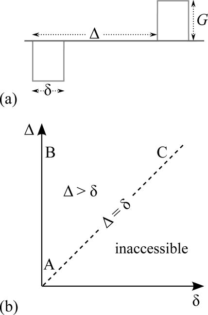
(a) Stejskal and Tanner’s pulsed field gradient experiment features a pair of rectangular gradient pulses of duration δ whose leading edges are separated by Δ. (b) The timing parameters of this experiment lie on or above the dashed line since the separation of the two pulses (Δ) has to be at least as long as the duration of each of them (δ). Thus, the experiment has three distinct regimes (labeled A, B, and C) based on whether these timing parameters are short or long. These are the three regimes that exhibit all interesting features of the signal. The same features are expected to be observed to various degrees in the intermediate region between these three regimes.

Our focus in this work is the orientationally-averaged signal, which can be obtained by computing the “isotropic component” of the signal, as was referred to in [10] and actually estimated as a byproduct of the q-space signal representation in [11]. Alternatively, the signal values measured over all gradient directions at a particular q-value can be averaged [12, 13] so that any dependence on the direction of the gradient vector is lost. Repeating this procedure for all q-values reduces the data collected over the three-dimensional q-space into a one-dimensional profile, which does not contain any information on ensemble (macroscopic) anisotropy.² The estimated signal profile represents the decay for the so-called “powdered” specimen, which contains an isotropic distribution of each and every compartment in the original specimen [19, 20]. The orientationally-averaged signal for axisymmetric compartments, each of which contributes according to (1), is thus the same as the signal for an isotropic ensemble of such compartments, and is given by [21, 6, 22]

$$\overline{E}\left(q\right)=\frac{\sqrt{\pi }{e}^{-q^2{v}_{\perp }}\text{erf}\left(q\sqrt{v_{\Vert }-v_{\perp }}\right)}{2q\sqrt{v_{\Vert }-v_{\perp }}}.$$ (2)

This expression predicts a squared exponential decay in general. However, if signal loss is limited to only the fiber direction (v_⊥ = 0), a much slower decay emerges. A power law of the form Ē ∝ q⁻¹, to be specific. Therefore, the appearance of this particular power-law can be used as an indicator of vanishing transverse diffusivity, in other words, the signal decay tensor V being of rank 1. We note that the problem of characterizing the orientationally averaged signal is considerably more complicated when (1) cannot be used to represent the compartmental signal; addressing this issue is one of our goals in this study.

The Ē ∝ q⁻¹ decay alluded to above was recently reported in white matter [1, 23]. These studies have found that in white-matter-dominated regions of the brain, the orientationally averaged signal exhibits a decay ∼ q^−c with an exponent c close to 1, in support of cylindrical neural projections as remarked above. In gray-matter-dominated regions, McKinnon et al. [1] have observed a larger exponent c ≈ 1.8 ± 0.2. They proposed that the apparent breakdown of the cylinder model may indicate a significantly larger permeability of the cellular membranes in gray matter versus white matter. Here, we investigate an alternative hypothesis. Namely, the departure of the exponent c from 1 can well be due to impermeable but curved projections. To assess this point, we studied the influence of neural projections’ size and shape on the orientationally-averaged diffusion MR signal. Due to the large variability in the geometric features of the neural cells, all temporal regimes of the Stejskal-Tanner sequence were considered, and the problem was studied both in the small-q regime as well as at larger q-values for which (1) and thus (2) are inaccurate.

Investigation of power-like tails in the diffusion MR signal go back to Köpf et al. [24], where large values of the wave vector were achieved using a fringe field method. A range of exponents (roughly between −1.8 and −4.6) were observed across various nonneural tissue types, as well as stretched exponential behavior, which was ascribed to fractional Brownian motion. In a subsequent study, Yablonskiy et al. [25] predicted an exponent of −2 for specimens featuring compartments with a distribution of diffusivities. Jian et al. [26] considered a parametric tensor distribution, which suggested a signal decay with a general power-law tail. These studies, however, observe or predict the signal decay for measurements along a single direction. As for the orientationally (powder) averaged signal, a quite general statement regarding an asymptotic power-law decay in the diffusion MR signal is the Debye-Porod law [27]. Here, the orientationally averaged signal measured using narrow pulses is predicted to follow a q⁻⁴ tail under quite general considerations. In our discussion, we take up apparent violations of this.

Although the influence of fiber curvature on the MR signal has been considered [28, 29, 30, 31, 32, 33] in various contexts, to our knowledge, this is the first study to provide explicit expressions for the signal decay for diffusion along a general parametrized curve and study its effect on the orientationally averaged signal.

In the next section, we provide explicit expressions for the MR signal for diffusion on curves in three distinct temporal regimes of the Stejskal-Tanner measurement. In the subsequent section, we discuss the implications of our theoretical findings as they relate to the morphology of neural cells and recent experimental observations. The article is concluded following a brief discussion of what observed power-law tails in the powder averaged signal may represent in that context, as well as from the perspective of the Debye-Porod law.

2 COMPARTMENTAL AND ORIENTATIONALLY-AVERAGED SIGNAL FOR DIFFUSION ALONG CURVES

The effective gradient waveform of a traditional Stejskal-Tanner measurement is shown in Figure 1a. In this work, we consider three distinct regimes of this pulse sequence based on whether δ and Δ are short or long. These regimes are indicated by the letters A, B, and C on the δ-Δ plane in Figure 1b. We note that the essential features of the signal at these three extreme situations are exhibited to some extent for more general timing values, i.e., within the interior of the triangle whose vertices are at A, B, and C.

The relevant size parameters of a simplified neural projection (ignoring branchings and other features such as beading patterns [34]) are: its contour length denoted by ℓ, its radius of gyration R_g, its characteristic curvature radius R_c, and the radius of the projection’s cross-section R₀. These parameters are illustrated for a representative projection in Figure 2. As mentioned in Introduction, R₀ is typically so small that qR₀ ≪ 1 for clinical MRI; this justifies representing the neurites and glial projections via one-dimensional curves. Thus, we shall consider diffusion taking place on a curve r(s) = (r₁(s), r₂(s), r₃(s))^⊤ parameterized by its arclength s, where 0 ≤ s ≤ ℓ.

Figure 2.

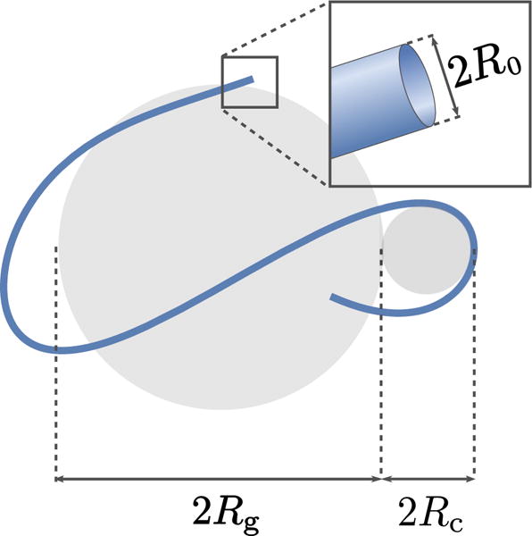
The relevant size parameters of a simplified neural projection (ignoring branchings and other features such as beading patterns [34]) are: its contour length denoted by ℓ, its radius of gyration R_g, the characteristic radius of curvature R_c, and the radius of the projection’s cross-section R₀.

2.1 Regime A: Short diffusion-time

In the first case, diffusion is observed for such a short time that the hindrances have not been encountered. This condition implies that the pulse durations are short as well. In fact, when $D\mathrm{\Delta }\ll R_c^2$, spins spread so little that even the most curved point along the projection seems like a straight segment.³ Thus, the compartmental signal occurs as the average, over the curve, of the signals originating from the tangents of the curve:

$$E\left(\mathit{q}\right)=\frac{1}{\mathcal{l}}{\displaystyle {\int }_0^{\mathcal{l}}\mathrm{d}s{e}^{-D\mathrm{\Delta }{\mathit{q}}^{\top }\widehat{\mathit{t}}\left(s\right){\widehat{\mathit{t}}}^{\top }\left(s\right)\mathit{q}}},$$ (3)

where

$$\widehat{\mathit{t}}\left(s\right)=\frac{\mathrm{d}\mathit{r}\left(s\right)}{\mathrm{d}s}$$ (4)

is the unit tangent to the curve.

As shown in Appendix A, the very small-q behavior of the orientationally-averaged signal (q²DΔ ≪ 1) is given by $\overline{E}\left(q\right)\approx e^{-q^{2}D\mathrm{\Delta }/3}$. Thus, the decay rate is determined solely by the (intracellular) diffusivity, and bears no geometric feature of the neural arborization in this regime.

For a more general analysis involving larger q-values, one can still employ (1) and (2) as follows. We are interested in the orientational average of the compartmental signal in (3), i.e.,

$$\overline{E}\left(q\right)=\frac{1}{\mathcal{l}}{\displaystyle {\int }_0^{\mathcal{l}}\mathrm{d}s}\langle e^{-D\mathrm{\Delta }{\mathit{q}}^{\top }\widehat{\mathit{t}}\left(s\right){\widehat{\mathit{t}}}^{\top }\left(s\right)\mathit{q}}\rangle ,$$ (5)

where the order of integration and orientational averaging, indicated by the angular brackets, was changed. However, the expression within the angular brackets is of the Gaussian form (1) with a rank-1 decay tensor whose non-vanishing eigenvalue is DΔ. Consequently, the signal for the powdered specimen is given through (2) by setting v_⊥ = 0, and v_║ = DΔ to be

$$\overline{E}\left(q\right)=\frac{\sqrt{\pi }\text{erf}\left(q\sqrt{D\mathrm{\Delta }}\right)}{2q\sqrt{D\mathrm{\Delta }}}.$$ (6)

Clearly, for larger q-values, the orientationally-averaged signal decay in regime A is proportional to q⁻¹ irrespective of the shape of the curve as long as $R_c^2\gg D\mathrm{\Delta }$. It can be observed that (5) has the form of a signal arising from a uniform orientational distribution of “sticks”. Hence the emergence of q⁻¹ at large q-values can be justified alternatively by Veraart et al.’s arguments [23].

Incorporating curvature effects

The above expression holds when the diffusion distance is much smaller than R_c as pointed out earlier. Here, we would like to generalize this expression to larger timing parameters, Δ and δ, to allow for the possibility that the diffusion distance during the course of the experiment is long enough for the molecules to traverse an approximately circular arc along the curve. Moreover, we assume that there is a single characteristic radius of curvature that represents the effective curvedness of the entire projection. This characteristic curvature is denoted by R_c.

Let $E_{\text{arc}}\left(\widehat{\mathit{n}},\phi ,\mathit{q}\right)$ denote the signal for a single such arc, where $\widehat{\mathit{n}}$ is the unit vector normal to its plane and φ is the polar coordinate of the center of the arc in a cylindrical reference frame oriented along $\widehat{\mathit{n}}$. The orientationally averaged signal can then be written as the average of $E_{\text{arc}}\left(\widehat{\mathit{n}},\phi ,\mathit{q}\right)$, over all possible realizations of a single arc, i.e.,

$$\overline{E}\left(q\right)=\frac{1}{4\pi }{\displaystyle {\int }_{S_2}\mathrm{d}\widehat{\mathit{n}}\frac{1}{2\pi }}{\displaystyle {\int }_0^{2\pi }\mathrm{d}\phi E_{\text{arc}}\left(\widehat{\mathit{n}},\phi ,\mathit{q}\right)},$$ (7)

where S₂ denotes the unit sphere. The second average simply defines the signal for a full circle of radius R_c. If we denote by $E_{\text{circ}}\left(\widehat{\mathit{n}},\mathit{q}\right)$ the signal for such a circle whose plane has the normal vector $\widehat{\mathit{n}}$, the orientationally averaged signal can be expressed as

$$\overline{E}\left(q\right)=\frac{1}{4\pi }{\displaystyle {\int }_{S_2}\mathrm{d}\widehat{\mathit{n}}{E}_{\text{circ}}\left(\widehat{\mathit{n}},\mathit{q}\right)}.$$ (8)

Due to its axial symmetry, the signal for the circle has the functional dependence $E_{\text{circ}}\left(\widehat{\mathit{n}}·\widehat{\mathit{q}},q\right)$, where $\widehat{\mathit{q}}=\mathit{q}/q$. Since $\widehat{\mathit{n}}·\widehat{\mathit{q}}$ is invariant under exchange of the unit vectors $\widehat{\mathit{n}}$ and $\widehat{\mathit{q}}$, one is free to replace the integration variable above with $\widehat{\mathit{q}}$ and fix $\widehat{\mathit{n}}$ instead [19]. With the variable θ defined through $\widehat{\mathit{n}}·\widehat{\mathit{q}}=\text{cos}\theta$, we moreover note that since there is no motion and hence no signal attenuation in the direction along $\widehat{\mathit{n}}$, the integrand’s functional dependence may further be reduced to E_circ(q sin θ), namely, the signal obtained when a q-vector of magnitude q sin θ is applied in the plane of the circle. Upon taking these observations into account, we obtain

$$\overline{E}\left(q\right)={\displaystyle {\int }_0^{\pi /2}\mathrm{d}\theta \sin \theta E_{\mathit{circ}}\left(q\sin \theta \right)}.$$ (9)

Narrow pulses

First, we shall consider the scenario involving narrow pulses, i.e., $D\delta \ll R_c^2$ but allow for the possibility that $D\mathrm{\Delta }\approx R_c^2$. For arbitrary Δ, the signal for a full circle is given by [28]

$$E_{\text{circ}}\left(q\right)=J_0{\left(q{R}_c\right)}^2+2{\displaystyle \sum _{n=1}^{\mathrm{\infty }}{e}^{-n^{2}D\mathrm{\Delta }/R_c^2}{J}_n{\left(q{R}_c\right)}^2},$$ (10)

where J_n denotes the nth order Bessel function. This expression yields, via (9), the orientationally-averaged signal to be

$$\begin{gathered} \overline{E}\left(q\right)=J_0\left(2q{R}_c\right)+\frac{\pi }{2}\left[J_1\left(2q{R}_c\right){\mathit{H}}_0\left(2q{R}_c\right)-J_0\left(2q{R}_c\right){\mathit{H}}_1\left(2q{R}_c\right)\right] \\ +2{\displaystyle \sum _{n=1}^{\mathrm{\infty }}{e}^{-n^{2}D\mathrm{\Delta }/R_c^2}\frac{{\left(q{R}_c\right)}^{2n}}{\left(2n+1\right)!}}{}_1{F}_2\left(n+\frac{1}{2};n+\frac{3}{2},2n+1;-q^2{R}_c^2\right), \end{gathered}$$ (11)

where H_α is the Struve function of order α and ₁F₂ represents the generalized hypergeometric function. We note that this orientationally averaged signal in the narrow pulse regime has the asymptotic behavior

$$\overline{E}\left(q\right)~\frac{\sqrt{\pi }\text{erf}\left(q\sqrt{D\mathrm{\Delta }}\right)}{2q\sqrt{D\mathrm{\Delta }}}+\frac{{\left(D\mathrm{\Delta }\right)}^2{q}^2{e}^{-D\mathrm{\Delta }{q}^2}}{6R_c^2}-\mathcal{O}\left(R_c^{-4}\right).$$ (12)

This expression contains the curvature-related correction to (6), which is valid for straight fibers, and suggests that curvature induced effects are rather limited for the case of narrow pulses, as the Ē(q) ∝ q⁻¹ dependence is unaffected at larger q-values.

Longer pulse durations

To investigate the influence of longer pulse durations, we numerically evaluated the integral in (9) using Simpson’s rule [35]. We adapted the multiple correlation (MCF) framework to the problem of diffusion on a circle. The details of this procedure are provided in Appendix B.

In Figure 3, we illustrate the signal decay curves at different pulse durations. In these simulations, the DΔ value was set equal to $R_c^2$; during a time interval of duration Δ, the spread of molecules on the circle is about 80°. When the pulse duration is short, we verified that the decay obeys the expressions in (11) and (12) (results not shown). The power-law, E(q) ∝ q⁻¹, which is valid in the narrow pulse regime does not prevail when the pulses are prolonged.

Figure 3.

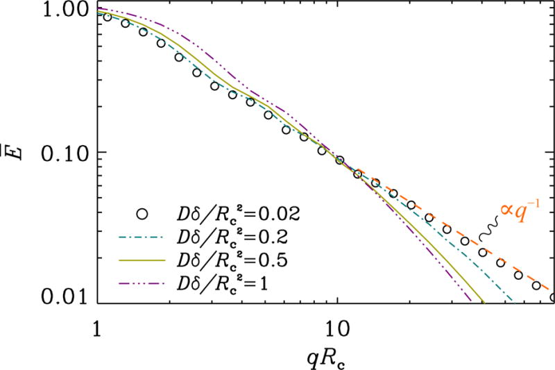
Signal attenuation curves for different values of the pulse duration. The separation of pulses was taken so that $D\mathrm{\Delta }=R_c^2$. The q⁻¹ decay, visible at short pulse durations, disappears as the pulses are prolonged.

2.2 Regime B: Long diffusion-time and narrow pulses

When diffusion is probed via a pair of impulses (or, when $D\delta \ll R_c^2$) separated from each other by a duration long enough for the molecules to reach all points within the curve, i.e., DΔ ≫ ℓ², the signal is given simply by the expression $E\left(\mathit{q}\right)={\left|\stackrel{\sim }{\rho }\left(\mathit{q}\right)\right|}^2$, where $\stackrel{\sim }{\rho }\left(\mathit{q}\right)$ is the Fourier transform of the density

$$\rho \left(\mathit{r}\right)=\frac{1}{\mathcal{l}}{\displaystyle {\int }_0^{\mathcal{l}}\mathrm{d}s\delta \left(\mathit{r}-\mathit{r}\left(s\right)\right)},$$ (13)

which is uniform along the curve. The orientationally averaged signal decay is thus obtained by averaging ${\left|\stackrel{\sim }{\rho }\left(\mathit{q}\right)\right|}^2$, and is given by

$$\overline{E}\left(q\right)=\frac{1}{{\mathcal{l}}^2}{\displaystyle {\int }_0^{\mathcal{l}}\mathrm{d}s}{\displaystyle {\int }_0^{\mathcal{l}}\mathrm{d}{s}^{\prime }}\frac{\sin \left[q\left|\mathit{r}\left(s\right)-\mathit{r}\left(s^{\prime }\right)\right|\right]}{q\left|\mathit{r}\left(s\right)-\mathit{r}\left(s^{\prime }\right)\right|}.$$ (14)

This expression is referred to as the Debye scattering equation [36], which is widely utilized in studies employing small angle scattering experiments for characterizing the structure of polymers. The essential features of the resulting Ē(q) curve are well-understood [37, 38]. As shown in Appendix A, the small-q regime (qR_g ≪ 1, the “Guinier regime” of scattering experiments) is described by the relationship $\overline{E}\left(q\right)\approx e^{-{\left(q{R}_g\right)}^2/3}$. As for larger q-values, such studies indicate that depending on the structure of the polymer, different sections of the curve could be characterized by different power-laws. For example, Gaussian chains undergo q⁻² decay, while fractional exponents are obtained for curves exhibiting fractality. Perhaps the most relevant finding, however, is that wormlike structures (i.e., those characterized by a so-called persistence length over which the polymer is likely to retain its direction) are characterized by a decay ∝ q⁻¹ at q-values about the reciprocal of the chain’s persistence length [39]. Thus, even a class of non-straight structures exhibit q⁻¹ decay in Regime B.

2.3 Regime C: Long pulse-duration

For the traditional Stejskal-Tanner measurement utilizing a pair of identical pulses in opposite directions, the compartmental signal has the form

$$E={\langle e^{-iq·\left({\mathit{\xi }}_2-{\mathit{\xi }}_1\right)}\rangle }_{\text{paths}},$$ (15)

where the averaging is performed over all trajectories, with

$${\mathit{\xi }}_n=\frac{1}{\delta }{\displaystyle {\int }_{t_n}^{t_n+\delta }\mathit{r}(t)}\mathrm{d}t$$ (16)

is the center of mass coordinate [40] of the fragment of trajectory coinciding with each pulse (t₁ = 0 and t₂ = Δ). Therefore, the MR signal (15) elicited by flat gradient pulses is not sensitive to the Brownian trajectories instant by instant but only in a time averaged sense.

In the limit Dδ/ℓ² → ∞, the two random variables lose correlation and the explicit dependence on Δ disappears, leading to the signal intensity [40]

$$E={\left|{\stackrel{\sim }{p}}_{\text{cm}}\left(\mathit{q},\delta \right)\right|}^2,$$ (17)

where

$${\stackrel{\sim }{p}}_{\text{cm}}\left(\mathit{q},\delta \right)={\displaystyle \int p_{\text{cm}}}\left(\mathit{\xi },\delta \right)e^{-iq·\mathit{\xi }}\mathrm{d}\mathit{\xi }$$ (18)

is the Fourier transform of the center of mass distribution. Moreover, in this limit, the distribution for the random variable ξ approaches a Gaussian due to the central limit theorem [41]⁴. Consequently, the signal (17) also approaches a quadratic exponential form, encoding no more structural information than the variance of p_cm(ξ, δ). Whether the domain is an irregularly curved fiber or a much more regular shape like a sphere, its fine structural features will find no representation in the signal acquired this way, since the length of the time averaging (pulse) has suppressed all short-scale (high q) variation encoded in the cumulants higher than the second.

Hence, the compartmental signal has the form (1). Here, though, V is the variance tensor for the center of mass coordinate (16) for a trajectory of (long) duration δ. This variance can be calculated for diffusion along a general continuous curve following Mitra and Halperin’s [40] derivation in the case of slab geometry, with slight modifications. One finds

$$V_{ij}=\frac{2}{D\delta }{\displaystyle {\int }_0^{\mathcal{l}}\mathrm{d}s{r}_i\left(s\right)}{\displaystyle {\int }_0^{\mathcal{l}}\mathrm{d}{s}^{\prime }{r}_j\left(s^{\prime }\right)}\left\{B_2\left(\frac{\left|s-s^{\prime }\right|}{2\mathcal{l}}\right)+B_2\left(\frac{s+s^{\prime }}{2\mathcal{l}}\right)+\frac{{\mathcal{l}}^2}{3D\delta }\left[B_4\left(\frac{\left|s-s^{\prime }\right|}{2\mathcal{l}}\right)+B_4\left(\frac{s+s^{\prime }}{2\mathcal{l}}\right)\right]\right\},$$ (19)

where B_n(·) denotes the nth order Bernoulli polynomial, and Dδ/ℓ² ≫ 1. Here, the exponentially decaying terms are ignored as their contribution is negligible at even moderate durations. The details of the derivation of the above expression is provided in Appendix A. We note that alternative representations of the final result (19) can be given in terms of polylogarithmic or Hurwitz zeta functions. We verified that (19) correctly reproduces Mitra and Halperin’s expression [40] in the same regime for the slab geometry, i.e., for a straight line.

As were in the previous cases, the signal decay tensor for long pulse duration is not rank-1 for a general curve. However, unlike in previous regimes, the compartmental signal decay is truly Gaussian. Consequently, the orientationally averaged signal in this regime suffers q⁻¹ decay if and only if the fibers are straight.

3 RESULTS AND DISCUSSION

Summary

The above findings can be summarized as follows: For narrow pulses $\left(D\delta \ll R_c^2,{\mathcal{l}}^2\right)$ in regimes A and B, the orientationally averaged signal exhibits a slow q⁻¹ tail for large q for diffusion along curved as well as straight 1 dimensional structures. As the pulse duration is prolonged, as we have studied for regime A, the slow q⁻¹ tail gives way to a steeper drop for substantially curved fibers, by which we mean $R_c\lesssim \sqrt{D\delta }$. Indeed, the signal may be expected to bear less features of diffusion along a 1D structure and more of diffusion in a 3D domain (i.e., a steep decay), since a long pulse serves to average the motion of the spin carriers over a length $~\sqrt{D\delta }$ along the path curved in 3D space. Fibers much shorter than the averaging length $\left(\mathcal{l}\ll \sqrt{D\delta }\right)$ fall into regime C and may contribute to an exponent of −1 in the orientationally averaged signal only if they are straight (R_c ≫ ℓ).

Clinical relevance

An important question to ask is: What regime is the most relevant for clinical MR examinations of the brain? There is no clear answer to this question, essentially because of the extremely wide variability in the size and shapes of cells within the brain [44]⁵. Consequently, it is impossible to suggest that diffusion within all neural cells takes place in a single experimental regime. We can, nonetheless, argue that regime B is the least relevant one as it is impossible to meet the narrow pulse condition along with long diffusion time condition when δ ≈ Δ as in clinical acquisitions performed at larger (in a practical sense) b-values, where b = q²(Δ − δ/3). The diffusion distance $\sqrt{2D\mathrm{\Delta }}$ is expected to be about 10-20 μm in such acquisitions, which will place longer $\left(\mathcal{l}\gg \sqrt{D\mathrm{\Delta }}\right)$ arborizations toward regime A while the shorter $\left(\mathcal{l}\gg \sqrt{D\mathrm{\Delta }}\right)$ ones will tend to exhibit features of regime C. If the longer structures furthermore exhibit curvature radii safely above the “averaging length” $\left(R_c\gg \sqrt{D\delta }\right)$, the q⁻¹ signature will be possible to observe over a range of large q-values without requiring strict straightness, as demonstrated in Fig. 3. For structures whose radii of curvature are small $\left(R_c\lesssim \sqrt{D\delta }\right)$ the appearance of the slow decay q⁻¹ becomes sensitive to curvature, and is not retained for as wide a range of q-values (see Fig. 4). At the extreme end of the spectrum, for structures so short that $\mathcal{l}\gg \sqrt{D\delta }$, entering into regime C, no curvature is tolerated if the tail q⁻¹ is to appear. These considerations will have to be revisited if one measures the diffusion of molecules other than water, due to differences in their diffusion characteristics [48, 49, 50].

Figure 4.

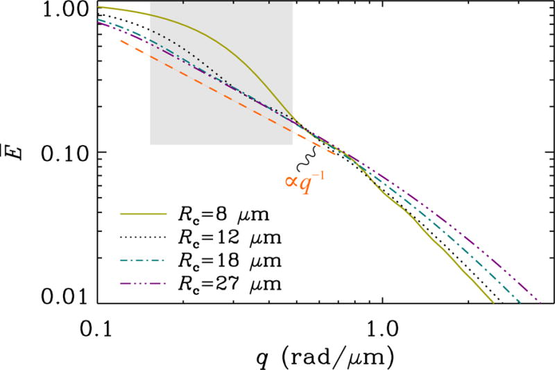
Simulation of the orientationally averaged signal for diffusion along an arc of various curvature radii. The contour length was taken to be infinite so that the results for Regime A are employed. The timing parameters were taken to be clinically realistic for high b-value acquisitions (δ = 50 ms and Δ = 60 ms), and the diffusion coefficient was set to D = 3 μm²/ms. The gray box depicts roughly the range of b-values between 1-10 ms/μm². It is seen that the larger the curvature radius, the wider the range over which the exponent −1 can be observed. Conversely, below a cutoff determined by the averaging length $\sqrt{D\delta }$, a steeper decay of the signal becomes very prominent.

On experimental findings

In light of the above deliberations, we can revisit the experimental observations of McKinnon et al. [1] who have reported the powder averaged signals stemming from various brain regions dominated by white- or gray-matter. In white-matter regions, they have measured a decay q^−c for large q with c values in the neighborhood c ≈ 1.1 ± 0.1, whereas in gray-matter regions, the decay was significantly faster, with c ≈ 1.8 ± 0.2. Concerning the faster decay observed in gray-matter, they propose an explanation based on permeability differences in white and gray-matter regions. If one assumes impermeable membranes, as we did in this study, the following alternative interpretation seems adequate: In white-matter, the observation of the tail q⁻¹ is compatible with regimes A and C, suggesting a substantial presence of fibers that fall into these regimes. The former implies long fibers $\left(\mathcal{l}\gg \sqrt{D\mathrm{\Delta }}\right)$ that could in fact be modestly curved (as long as $R_c\gg \sqrt{D\delta }$ remains valid). The latter implies short fibers $\left(\mathcal{l}\gg \sqrt{D\delta }\right)$ that are straight. In gray-matter regions, the loss of the slow q⁻¹ decay suggests that the signal originates predominantly from fibers that fall outside these descriptions, i.e., exhibiting strong curvature $\left(R_c\lesssim \sqrt{D\delta }\right)$. Indeed, gray-matter is rich in dendrites and unmyelinated axons, which will exhibit a fair amount of bending distributed across any voxel. The gray box in Fig. 4 depicts roughly the q range used in McKinnon et al.’s study, where it is seen that while modest curvatures do exhibit the exponent −1 for a while, strong curvature yields a steeper decay for most of the range.

Another potential explanation involves the glial cells, which constitute a substantial portion of all neural cells. Similar to neurons, glial cells exhibit an extraordinary level of diversity in their size and shape throughout the brain. Their relative number and distribution is the subject of ongoing debate [51]. Thus, an accurate assessment of their influence on the detected diffusion MR signal is infeasible at this time. It is known, however, that the glial cells tend to be smaller than neurons, they lack axons, and many of them are star-shaped [52]. These structural features tend to disfavor the emergence of a q⁻¹ decay. However, recent studies have suggested that the glial cells are significantly more prevalent in cerebral white-matter compared to gray-matter [53]. Thus, it can be argued that their contribution to the overall MR signal must be rather limited. We note that the vast variation in neuronal and glial morphology along with the reported regional differences justify future studies performed at high spatial resolutions, for understanding the influence of compositional variations on the diffusion MR signal.

Immobile water

The detected orientationally-averaged signal would typically include contributions from many different compartments besides the neural projections, including extracellular matrix, cell bodies, and molecules trapped within very small regions (e.g., within certain organelles, between myelin layers, etc.). Among these, molecules diffusing relatively freely (for instance, between the neural processes) are expected to yield a decay rate faster than q⁻¹ so that much of their contribution is expected to disappear at larger q values. Conversely, there would be no significant loss of signal for truly restricted particles. Presence of a substantial portion of signal originating from such compartments as well as noise-induced bias associated with employing magnitude-valued data would make the decay appear slower [54, 55] than q⁻¹. The decay exponent c ≈ 1.1 ± 0.1 reported by McKinnon et al. [1] suggests that contributions from such immobile spins could be negligible in their acquisitions. This can be attributed [23] to the relatively short transverse relaxation times those spins are expected to have, along with the long echo times employed at larger q-value acquisitions via clinical scanners.

A possible error

One may be tempted to employ (1) for the compartmental signal, as it always has a Gaussian form for sufficiently small q values, and then to attribute the emergence of the q⁻¹ behavior of the orientationally averaged signal through (2) to the rank of the decay tensor V being 1. However, this may be permissible for large q only in regime C. This attribution would therefore be erroneous for large q in regimes A and B. Specifically, in regimes A and B, the q range in which (1) applies is similar to the q range in which the orientational average (2) exhibits a Gaussian tail no matter the rank of the tensor V (see Appendix A). Thus, the q⁻¹ behavior is not a consequence of the signal decay tensor having rank 1. Importantly, such behavior naturally emerges at larger q-values in regimes A and B for reasonable shapes of neural projections.

Debye-Porod Law

The powder averaged signal may be envisioned as having originated from a porous specimen which is macroscopically isotropic, in which case one expects an asymptote of the form q⁻⁴ due to the Debye-Porod law [27] (see Appendix C), while a steeper decay is predicted for longer pulses as the process approaches a Gaussian (see Appendix C). Since this behavior arises from quite general considerations, the observation of a tail of q⁻¹ appears questionable. Indeed, the observed power is most likely valid only in an intermediate range, as opposed to the strict q → ∞ limit. The asymptotic expansion, whose leading term gives the Debye-Porod law, contains terms that decay faster than any pure power (e.g., exponential). These terms may very well exhibit decays slower than q⁻⁴ over a certain stretch of q-values, before the Debye-Porod asymptote takes over, which happens when q begins to compete with the inverse length of the smallest dimension of the pore geometry. Alas, the q values used in McKinnon et al.’s experiments are of the order 0.1 μm⁻¹ which is far from large enough compared to the inverse length scale of 1 μm⁻¹ afforded by the axon diameter.

Unaccounted factors

One of the hallmarks of neuronal morphology is the axonal and dendritic branchings [56], which are not accounted for in our treatment of diffusion on curves. Although an accurate assessment of the influence of branchings could be achieved via careful numerical studies [57], the insight gained from our description above can be employed to some extent for making some predictions. For long structures, each branch can be considered a separate segment along which diffusion takes place. Thus, the presence of branchings would not impact the formulation for projections in regime A. However, since the total contour length can be considerably increased in the presence of branchings, it may be more difficult to satisfy the long pulse duration condition of regime C. When this condition is met, however, the rank of the signal decay tensor would almost certainly be greater than one. In other words, detecting q⁻¹ decay in regime C would be nearly impossible for smaller cells unless most arborizations run parallel within a narrow cylindrical region.

The detected MR signal is known to be dependent on factors other than those accounted for in this work. Among these, spatial heterogeneity of magnetic susceptibility within the tissue have been reported to influence the diffusion decay [58, 59] as well. In fact, suppressing [60] or taking advantage [61, 62] of effects due to susceptibility variations is an active area of research. We note that the presence of internal gradients could be investigated as yet another mechanism that could explain the reported features in the orientationally averaged signal; doing so would require an extension of existing studies relating the diffusion MR signal to microscopic perturbations in susceptibility [63, 64].

4 CONCLUSION

In an attempt to interpret new experimental findings, we studied the influence of diffusion along parameterized curves on orientationally-averaged diffusion MR signal. We examined the problem in three distinct temporal regimes of the Stejskal-Tanner experiment and investigated the appearance of a slow decay. We have found that for smaller cells, the q⁻¹ decay of the orientationally-averaged signal is predicted only for straight fibers. This decay is more general for cells with longer projections, while it fades away for curvy structures as the pulse duration of the gradient sequence increases. Finally, we stressed that the q⁻¹ decay could represent an intermediate range as the true asymptotic behavior is governed by the Debye-Porod law, which suggests the power-law, q⁻⁴. The findings of this paper are expected to provide insight into the link between the diffusion weighted MR acquisitions and geometry of the neural cells.

APPENDIX A: DERIVATIONS FOR THE SIGNAL DECAY TENSORS

Here, we provide the derivations of the signal decay tensors, V, for regimes A, B, and C, respectively. Fig. 5 illustrates the decay tensors as ellipses for an examplary selection of planar curves.

Figure 5.

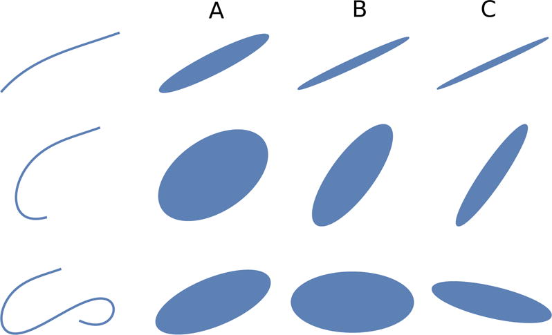
Figure showing three planar curves (left column), and ellipses depicting the signal decay tensor in the three regimes A, B, and C (see equations (21), (25), and (19)) considered. Here, the ellipses for the tensors were rescaled so as to produce a depiction of the same size.

Regime A and $\mathit{D}\mathbf{\Delta }\ll {\mathit{R}}_{\mathit{c}}^{\mathbf{2}}$

For small values of q²DΔ, the exponent in (3) is small, so the expression can be rewritten to leading order, by moving the averaging integral into the exponent, as

$$E\left(\mathit{q}\right)\approx e^{-D\mathrm{\Delta }\frac{1}{\mathcal{l}}{\displaystyle {\int }_0^{\mathcal{l}}\mathrm{d}s{\mathit{q}}^{\top }\widehat{\mathit{t}}\left(s\right){\widehat{\mathit{t}}}^{\top }\left(s\right)\mathit{q}}}.$$ (20)

In this small-q regime, the form $E\left(\mathit{q}\right)=e^{-{\mathit{q}}^{\top }\mathit{V}\mathit{q}}$ (1) identifies the decay tensor V_ij as

$$V_{ij}=\frac{D\mathrm{\Delta }}{\mathcal{l}}{\displaystyle {\int }_0^{\mathcal{l}}\mathrm{d}s}\frac{\mathrm{d}{r}_i\left(s\right)}{\mathrm{d}s}\frac{\mathrm{d}{r}_j\left(s\right)}{\mathrm{d}s}.$$ (21)

The integrand in the above expression is a rank-1 tensor by construction. For a general curve, the integral mixes together different rank-1 tensors resulting in a V_ij of higher rank, the only exception being a straight line. Note that since dr/ds is a unit vector, the trace of the above matrix is DΔ. The orientationally-averaged signal (2) in the small q²DΔ regime is just $\overline{E}\left(q\right)\approx e^{-q^2\mathrm{T}r\mathit{V}/3}=e^{-q^{2}D\mathrm{\Delta }/3}$.

Regime B

The three-dimensional Fourier transform of the spin density (13) is given by

$$\stackrel{\sim }{\rho }\left(\mathit{q}\right)=\frac{1}{\mathcal{l}}{\displaystyle {\int }_0^{\mathcal{l}}\mathrm{d}s{e}^{-i\mathit{q}·\mathit{r}\left(s\right)}},$$ (22)

which is substituted into $E\left(\mathit{q}\right)={\left|\stackrel{\sim }{\rho }\left(\mathit{q}\right)\right|}^2$, yielding the signal decay

$$E\left(\mathit{q}\right)=\frac{1}{{\mathcal{l}}^2}{\displaystyle {\int }_0^{\mathcal{l}}\mathrm{d}s}{\displaystyle {\int }_0^{\mathcal{l}}\mathrm{d}{s}^{\prime }{e}^{-i\mathit{q}·\left[\mathit{R}\left(s\right)-\mathit{R}\left(s^{\prime }\right)\right]}}.$$ (23)

In this expression, we employed the change of variables R(s) = r(s) − R_cm, where R_cm is the center of mass of the curve. For small q values, the exponential can be replaced by its Maclaurin series up to quadratic order. Term-by-term evaluation of the double integral then yields

$$\begin{gathered} E\left(\mathit{q}\right)\approx 1-\frac{1}{\mathcal{l}}{\displaystyle {\int }_0^{\mathcal{l}}\mathrm{d}s}{\left[\mathit{q}·\mathit{R}\left(s\right)\right]}^2 \\ \approx \exp \left(-\frac{1}{\mathcal{l}}{\displaystyle {\int }_0^{\mathcal{l}}\mathrm{d}s{\mathit{q}}^{\top }\mathit{R}\left(s\right)\mathit{R}{\left(s\right)}^{\top }\mathit{q}}\right), \end{gathered}$$ (24)

which leads to the identification of the signal decay tensor given by

$$V_{ij}=\frac{1}{\mathcal{l}}{\displaystyle {\int }_0^{\mathcal{l}}\mathrm{d}s{R}_i\left(s\right)R_{ij}\left(s\right)}.$$ (25)

Like in the previous regime, V_ij is rank-1 only for straight fibers. The trace of the above matrix is $R_g^2$, by definition. The orientationally-averaged signal (2) in the small qR_g regime is then just $\overline{E}\left(q\right)\approx e^{-q^2\text{Tr}\mathit{V}/3}=e^{-{\left(q{R}_g\right)}^2/3}$.

Regime C

Similar to regime B, the signal decay tensor V_ij is the variance of a probability distribution; this time the center of mass distribution, p_cm(ξ, δ). Using the definition (16), the variance 〈ξ_iξ_j〉 − 〈ξ_i〉 〈ξ_j〉 can be calculated as

$$V_{ij}=\frac{2}{\mathcal{l}{\delta }^2}{\displaystyle {\int }_0^{\delta }\mathrm{d}{t}_1}{\displaystyle {\int }_{t_1}^{\delta }\mathrm{d}{t}_2}{\displaystyle {\int }_0^{\mathcal{l}}\mathrm{d}{s}_1}{\displaystyle {\int }_0^{\mathcal{l}}\mathrm{d}{s}_2{r}_i\left(s_1\right)r_j\left(s_2\right)}\left[P\left(s_2,t_2|s_1,t_1\right)-\frac{1}{\mathcal{l}}\right],$$ (26)

where [65]

$$P\left(s,t^{\prime }+t|s^{\prime },t^{\prime }\right)=\frac{1}{\mathcal{l}}+\frac{2}{\mathcal{l}}{\displaystyle \sum _{n=1}^{\mathrm{\infty }}{e}^{-\frac{n^2{\pi }^{2}Dt}{{\mathcal{l}}^2}}}\cos \frac{n\pi s}{\mathcal{l}}\cos \frac{n\pi s^{\prime }}{\mathcal{l}}$$ (27)

is the propagator from arc-length coordinate s′ to s in a time t. The time integrals in (26) are done easily, and after further dropping exponentially decaying temporal terms on account of Dδ ≫ ℓ², one obtains

$$V_{ij}=\frac{4}{{\pi }^{2}D\delta }{\displaystyle {\int }_0^{\mathcal{l}}\mathrm{d}{s}_1}{\displaystyle {\int }_0^{\mathcal{l}}\mathrm{d}{s}_2}{\displaystyle \sum _{n=1}^{\mathrm{\infty }}\left(\frac{1}{n^2}-\frac{{\mathcal{l}}^2}{{\pi }^2{n}^{4}D\delta }\right)}\cos \frac{n\pi s_1}{\mathcal{l}}\cos \frac{n\pi s_2}{\mathcal{l}}.$$ (28)

It turns out that the sum over n admits a closed form, which results in the final expression (19).

APPENDIX B: COMPUTING THE SIGNAL FOR DIFFUSION ON A CIRCLE

We employed the multiple correlation function (MCF) framework [66, 67, 68, 69] for estimating the signal attenuation due to diffusion taking place on a circle whose radius is denoted by R. This problem can be considered as the limiting case of the problem involving diffusion within circular layers of finite thickness [70].

The evolution of magnetization is governed by the Bloch-Torrey equation [71]. For our problem, it can be written as

$$\frac{\partial M}{\partial t}=\frac{D}{R^2}\frac{{\partial }^{2}M}{\partial {\varphi }^2}-i\gamma RG\left(t\right)\cos \varphi M\left(\varphi ,t\right),$$ (29)

where we assumed that the gradients are applied along the x direction. The MCF approach considers the eigenproblem

$$\frac{{\partial }^2{u}_k\left(\varphi \right)}{\partial {\varphi }^2}=-{\mathrm{\lambda }}_k{u}_k\left(\varphi \right)$$ (30)

along with the periodicity condition u_k(ϕ + 2π) = u_k(ϕ), which is valid for the circular geometry. The eigenvalues are simply k², while the eigenfunctions are u_k(ϕ) = (2π)^−1/2e^ikϕ, where k is any integer.

The MCF technique is based on expressing the problem of computing the signal attenuation in this eigenbasis. The two terms on the right hand side of (29) lead to two infinite-dimensional matrix operators, which we shall denote by Λ and A, respectively. The components of these operators are given by

$${\mathrm{\Lambda }}_{m,n}=n^2{\delta }_{m,n},\text{and}$$ (31)

$$A_{m,n}=\frac{1}{2}\left({\delta }_{m,n+1}+{\delta }_{m,n-1}\right).$$ (32)

The signal for a Stejskal-Tanner measurement is given simply by the element of the matrix

$$e^{-\mathbf{\Lambda }D\delta /R^2-\mathit{iqR}\mathit{A}}{e}^{-\mathbf{\Lambda }D\left(\mathrm{\Delta }-\delta \right)/R^2}{e}^{-\mathbf{\Lambda }D\delta /R^2+\mathit{iqR}\mathit{A}}$$ (33)

identified by the indices 0 and 0.

APPENDIX C: ON THE DEBYE-POROD LAW

For a bipolar pulsed gradient sequence, the signal E(q) is the Fourier transform of a displacement probability distribution, P (r), often referred to as the average propagator (between center of mass positions if pulses are of long duration [40]). When the specimen is macroscopically isotropic, e.g., if it consists of a uniform orientational distribution of identical compartments, the signal becomes

$$\overline{E}\left(q\right)=4\pi {\displaystyle {\int }_0^{\mathrm{\infty }}\mathrm{d}r}{r}^2\frac{\text{sin}\left(qr\right)}{qr}\overline{P}\left(r\right),$$ (34)

using the purely radial term in the spherical wave expansion of e^−iq·r, where $\overline{P}\left(r\right)={\left(4\pi \right)}^{-1}{\displaystyle \int \mathrm{d}\mathrm{\Omega }}P\left(\mathit{r}\right)$ is the orientational average of P (r). In the physics of scattering, this formula is identical to that of the scattered intensity originating from a dilute aggregation of randomly-oriented scatterers, with P (r) identified as the auto-correlation function of the scattering density in proper units [37, 38].

Depending on the analytical properties of the function $\overline{P}\left(r\right)$, it may be possible to develop the signal (34) into an asymptotic expansion in powers of q⁻¹. This is achieved by repeated integrations by parts, exploiting the trivial integral of the sine (or cosine) in the integrand, each repetition yielding (possibly) a term proportional to the next power of q⁻¹. For diffusion in a finite 3D compartment, this procedure is permissible and yields a leading term ~ q⁻⁴ as q → ∞, whose coefficient was shown to be related to the return-to-origin probability at the surface [27], which is a generalization of what is known as the Debye-Porod law in the field of scattering [37, 38]. This particular exponent of −4 is expected universally, when the measurement is done with a resolution (∼ q⁻¹) substantially finer than the smallest dimension of the compartment. Below this cutoff, the compartment will appear effectively lower dimensional, and Ē(q) may exhibit an appreciable stretch of q-values where it exhibits a slower power law decay, depending on the geometry. This is not in conflict with the Debye-Porod law, but simply outside its domain of applicability.

For lower dimensional objects, specific examples of rod and flat disk geometries indicate that $\overline{P}$ is of lower regularity. This means that the procedure of repeated integrations by parts either stops earlier or is even not applicable at all. As a consequence, the leading powers of q in the asymptotic expansion will not be −4, and for the 1D and 2D cases, [37], these leading powers were indeed found to be −1 and −2, respectively.

Gaussian pores

Given how universal the Debye-Porod law is, it may appear contradictory that the orientationally averaged signal (2) arising from 3D Gaussian compartments does not exhibit a q⁻⁴ decay, but rather a power q⁻¹ modulated by a decaying (quadratic) exponential.

To understand this, it is useful to consider more explicitly the asymptotic expansion of the signal (34), rearranged here slightly as,

$$\overline{E}\left(q\right)=\frac{4\pi }{q}{\displaystyle {\int }_0^{\mathrm{\infty }}\mathrm{d}r}\sin \left(qr\right)r\overline{P}\left(r\right).$$ (35)

As mentioned earlier, the asymptotic expansion procedure via integration by parts relies (to a certain extent) on the smoothness of the function $\overline{P}\left(r\right)$. In the Gaussian case where the displacement distribution $P\left(\mathit{r}\right)\propto e^{-\frac{1}{2}{\mathit{r}}^{\top }{\mathit{V}}^{-1}\mathit{r}}$, the orientational average $\overline{P}\left(r\right)$ has the same form as (2), but with different variables:

$$\overline{P}\left(r\right)\propto r^{-1}{e}^{-k_0^2{r}^2}\text{erf}\left(k_{1}r\right).$$ (36)

Thus, the natural extension (to the space of real numbers ℝ) of $r\overline{P}\left(r\right)$ is a smooth odd function which, together with all its derivatives, vanish at infinity. Repeated partial integration of (35) shows that for any even N,

$$\overline{E}\left(q\right)=\frac{4\pi }{q^2}{\displaystyle \sum _{n=0}^{N/2}{\left(\frac{-1}{q^2}\right)}^n}\frac{{\mathrm{d}}^{2n}}{\mathrm{d}{r}^{2n}}\left[r\overline{P}\left(r\right)\right]{|}_{r=0}+\frac{{\left(-1\right)}^{N/2}}{q^{N+2}}{\displaystyle {\int }_0^{\mathrm{\infty }}\mathrm{d}r}\cos \left(qr\right)\frac{{\mathrm{d}}^{N+1}}{\mathrm{d}{r}^{N+1}}\left[r\overline{P}\left(r\right)\right].$$ (37)

But since $r\overline{P}\left(r\right)$ is odd, all even derivatives vanish at r = 0. Hence, for any even N,

$$\left|\overline{E}\left(q\right)\right|\le \frac{1}{q^{N+2}}{\displaystyle {\int }_0^{\mathrm{\infty }}\mathrm{d}r}\left|\cos \left(qr\right)\frac{d^{N+1}}{d{r}^{N+1}}\left[r\overline{P}\left(r\right)\right]\right|\le \frac{C_N}{q^{N+2}}$$ (38)

for some constant C_N. This means that Ē(q) decays faster than any polynomial⁶. This observation implies that for truly Gaussian compartments [73] or long pulse acquisitions [43] (regime C), the asymptotic decay of Ē(q) should be faster than any polynomial, which is indeed true for the expression in Eq. (2).

References

- 1.McKinnon ET, Jensen JH, Glenn GR, Helpern JA. Dependence on b-value of the direction-averaged diffusion-weighted imaging signal in brain. Magn Reson Imaging. 2017;36:121–127. doi: 10.1016/j.mri.2016.10.026. [DOI] [PMC free article] [PubMed] [Google Scholar]
- 2.Assaf Y, Freidlin RZ, Rohde GK, Basser PJ. New modeling and experimental framework to characterize hindered and restricted water diffusion in brain white matter. Magn Reson Med. 2004;52:965–978. doi: 10.1002/mrm.20274. [DOI] [PubMed] [Google Scholar]
- 3.Stanisz GJ, Szafer A, Wright GA, Henkelman RM. An analytical model of restricted diffusion in bovine optic nerve. Magn Reson Med. 1997;37:103–111. doi: 10.1002/mrm.1910370115. [DOI] [PubMed] [Google Scholar]
- 4.Jespersen SN, Kroenke CD, Østergaard L, Ackerman JJH, Yablonskiy DA. Modeling dendrite density from magnetic resonance diffusion measurements. NeuroImage. 2007;34:1473–86. doi: 10.1016/j.neuroimage.2006.10.037. [DOI] [PubMed] [Google Scholar]
- 5.Behrens TEJ, Woolrich MW, Jenkinson M, Johansen-Berg H, Nunes RG, Clare S, et al. Characterization and propagation of uncertainty in diffusion-weighted MR imaging. Magn Reson Med. 2003;50:1077–88. doi: 10.1002/mrm.10609. [DOI] [PubMed] [Google Scholar]
- 6.Kroenke CD, Ackerman JJH, Yablonskiy DA. On the nature of the NAA diffusion attenuated MR signal in the central nervous system. Magn Reson Med. 2004;52:1052–9. doi: 10.1002/mrm.20260. [DOI] [PubMed] [Google Scholar]
- 7.Zhang H, Schneider T, Wheeler-Kingshott CA, Alexander DC. NODDI: practical in vivo neurite orientation dispersion and density imaging of the human brain. NeuroImage. 2012;61:1000–16. doi: 10.1016/j.neuroimage.2012.03.072. [DOI] [PubMed] [Google Scholar]
- 8.Stejskal EO, Tanner JE. Spin diffusion measurements: Spin echoes in the presence of a time-dependent field gradient. J Chem Phys. 1965;42:288–292. [Google Scholar]
- 9.Jensen JH. Sufficiency of diffusion tensor in characterizing the diffusion MRI signal to leading order in diffusion weighting. NMR Biomed. 2014;27:1005–1007. doi: 10.1002/nbm.3145. [DOI] [PubMed] [Google Scholar]
- 10.Özarslan E, Basser PJ. Microscopic anisotropy revealed by NMR double pulsed field gradient experiments with arbitrary timing parameters. J Chem Phys. 2008;128:154511. doi: 10.1063/1.2905765. [DOI] [PMC free article] [PubMed] [Google Scholar]
- 11.Özarslan E, Koay CG, Shepherd TM, Komlosh ME, İrfanoğlu MO, Pierpaoli C, et al. Mean apparent propagator (MAP) MRI: a novel diffusion imaging method for mapping tissue microstructure. NeuroImage. 2013;78:16–32. doi: 10.1016/j.neuroimage.2013.04.016. [DOI] [PMC free article] [PubMed] [Google Scholar]
- 12.Kaden E, Kruggel F, Alexander DC. Quantitative mapping of the per-axon diffusion coefficients in brain white matter. Magn Reson Med. 2016;75:1752–63. doi: 10.1002/mrm.25734. [DOI] [PMC free article] [PubMed] [Google Scholar]
- 13.Szczepankiewicz F, Westin CF, Knutsson H. A measurement weighting scheme for optimal powder average estimation. Proc Intl Soc Mag Reson Med. 2017;26:3345. [Google Scholar]
- 14.Mori S, van Zijl PC. Diffusion weighting by the trace of the diffusion tensor within a single scan. Magn Reson Med. 1995;33:41–52. doi: 10.1002/mrm.1910330107. [DOI] [PubMed] [Google Scholar]
- 15.Wong EC, Cox RW, Song AW. Optimized isotropic diffusion weighting. Magn Reson Med. 1995;34:139–43. doi: 10.1002/mrm.1910340202. [DOI] [PubMed] [Google Scholar]
- 16.Eriksson S, Lasič S, Topgaard D. Isotropic diffusion weighting in PGSE NMR by magic-angle spinning of the q-vector. J Magn Reson. 2013;226:13–18. doi: 10.1016/j.jmr.2012.10.015. [DOI] [PubMed] [Google Scholar]
- 17.Westin CF, Knutsson H, Pasternak O, Szczepankiewicz F, Özarslan E, van Westen D, et al. Q-space trajectory imaging for multidimensional diffusion MRI of the human brain. NeuroImage. 2016;135:345–62. doi: 10.1016/j.neuroimage.2016.02.039. [DOI] [PMC free article] [PubMed] [Google Scholar]
- 18.Lampinen B, Szczepankiewicz F, Møartensson J, van Westen D, Sundgren PC, Nilsson M. Neurite density imaging versus imaging of microscopic anisotropy in diffusion MRI: A model comparison using spherical tensor encoding. NeuroImage. 2017;147:517–531. doi: 10.1016/j.neuroimage.2016.11.053. [DOI] [PubMed] [Google Scholar]
- 19.Özarslan E. Compartment shape anisotropy (CSA) revealed by double pulsed field gradient MR. J Magn Reson. 2009;199:56–67. doi: 10.1016/j.jmr.2009.04.002. [DOI] [PMC free article] [PubMed] [Google Scholar]
- 20.Lawrenz M, Finsterbusch J. Double-wave-vector diffusion-weighted imaging reveals microscopic diffusion anisotropy in the living human brain. Magn Reson Med. 2013;69:1072–1082. doi: 10.1002/mrm.24347. [DOI] [PubMed] [Google Scholar]
- 21.Yablonskiy DA, Sukstanskii AL, Leawoods JC, Gierada DS, Bretthorst GL, Lefrak SS, et al. Quantitative in vivo assessment of lung microstructure at the alveolar level with hyperpolarized 3He diffusion MRI. Proc Natl Acad Sci U S A. 2002;99:3111–6. doi: 10.1073/pnas.052594699. [DOI] [PMC free article] [PubMed] [Google Scholar]
- 22.Anderson AW. Measurement of fiber orientation distributions using high angular resolution diffusion imaging. Magn Reson Med. 2005;54:1194–1206. doi: 10.1002/mrm.20667. [DOI] [PubMed] [Google Scholar]
- 23.Veraart J, Fieremans E, Novikov DS. Universal power-law scaling of water diffusion in human brain defines what we see with MRI. arXiv. 2016;1609:09145. [Google Scholar]
- 24.Köpf M, Corinth C, Haferkamp O, Nonnenmacher TF. Anomalous diffusion of water in biological tissues. Biophys J. 1996;70:2950–2958. doi: 10.1016/S0006-3495(96)79865-X. [DOI] [PMC free article] [PubMed] [Google Scholar]
- 25.Yablonskiy DA, Bretthorst GL, Ackerman JJH. Statistical model for diffusion attenuated MR signal. Magn Reson Med. 2003;50:664–9. doi: 10.1002/mrm.10578. [DOI] [PMC free article] [PubMed] [Google Scholar]
- 26.Jian B, Vemuri BC, Özarslan E, Carney PR, Mareci TH. A novel tensor distribution model for the diffusion-weighted MR signal. NeuroImage. 2007;37:164–176. doi: 10.1016/j.neuroimage.2007.03.074. [DOI] [PMC free article] [PubMed] [Google Scholar]
- 27.Sen PN, Hürlimann MD, de Swiet TM. Debye-Porod law of diffraction for diffusion in porous media. Phys Rev B. 1995;51:601–604. doi: 10.1103/physrevb.51.601. [DOI] [PubMed] [Google Scholar]
- 28.Özarslan E, Koay CG, Basser PJ. Remarks on q-space MR propagator in partially restricted, axially-symmetric, and isotropic environments. Magn Reson Imaging. 2009;27:834–844. doi: 10.1016/j.mri.2009.01.005. [DOI] [PubMed] [Google Scholar]
- 29.Nørhøj Jespersen S, Buhl N. The displacement correlation tensor: microstructure, ensemble anisotropy and curving fibers. J Magn Reson. 2011;208:34–43. doi: 10.1016/j.jmr.2010.10.003. [DOI] [PubMed] [Google Scholar]
- 30.Nilsson M, Lätt J, Støahlberg F, van Westen D, Hagslätt H. The importance of axonal undulation in diffusion MR measurements: a Monte Carlo simulation study. NMR Biomed. 2012;25:795–805. doi: 10.1002/nbm.1795. [DOI] [PubMed] [Google Scholar]
- 31.Reisert M, Kellner E, Kiselev VG. About the geometry of asymmetric fiber orientation distributions. IEEE Trans Med Imaging. 2012;31:1240–9. doi: 10.1109/TMI.2012.2187916. [DOI] [PubMed] [Google Scholar]
- 32.Pizzolato M, Wassermann D, Boutelier T, Deriche R. International Conference on Medical Image Computing and Computer-Assisted Intervention. Springer International Publishing; 2015. Exploiting the phase in diffusion MRI for microstructure recovery: Towards axonal tortuosity via asymmetric diffusion processes; pp. 109–116. [Google Scholar]
- 33.Cetin S, Özarslan E, Unal G. International Conference on Medical Image Computing and Computer-Assisted Intervention. Springer International Publishing; 2015. Elucidating intravoxel geometry in diffusion-MRI: asymmetric orientation distribution functions (AODFs) revealed by a cone model; pp. 231–238. [Google Scholar]
- 34.Budde MD, Frank JA. Neurite beading is sufficient to decrease the apparent diffusion coefficient after ischemic stroke. Proc Natl Acad Sci U S A. 2010;107:14472–7. doi: 10.1073/pnas.1004841107. [DOI] [PMC free article] [PubMed] [Google Scholar]
- 35.Press WH, Teukolsky SA, Vetterling WT, Flannery BP. Numerical Recipes in C: The Art of Scientific Computing. Cambridge: Cambridge Press; 1992. [Google Scholar]
- 36.Debye P. Zerstreuung der röntgenstrahlen. Ann Physik. 1915;46:809–824. [Google Scholar]
- 37.Glatter O, Kratky O, editors. Small Angle X-Ray Scattering. London: Academic Press; 1982. [Google Scholar]
- 38.Feigun LA, Svergun DI. Structure Analysis by Small-Angle X-Ray and Neutron Scattering. New York: Springer Science + Business Media; 1987. [Google Scholar]
- 39.des Cloizeaux J. Form factor of an infinite Kratky-Porod chain. Macromolecules. 1973;6:403–407. [Google Scholar]
- 40.Mitra PP, Halperin BI. Effects of finite gradient-pulse widths in pulsed-field-gradient diffusion measurements. J Magn Reson A. 1995;113:94–101. [Google Scholar]
- 41.Neuman CH. Spin echo of spins diffusing in a bounded medium. J Chem Phys. 1974;60:4508–4511. [Google Scholar]
- 42.Baxter JR, Brosamler GA. Energy and the law of the iterated logarithm. Math Scand. 1976;38:115–136. [Google Scholar]
- 43.Özarslan E, Yolcu C, Herberthson M, Westin CF, Knutsson H. Effective potential for magnetic resonance measurements of restricted diffusion. Front Phys. 2017;5:68. doi: 10.3389/fphy.2017.00068. [DOI] [PMC free article] [PubMed] [Google Scholar]
- 44.Schoonover C. Portraits of the Mind. New York, NY: Abrams; 2010. [Google Scholar]
- 45.Parekh R, Ascoli GA. Quantitative investigations of axonal and dendritic arbors: development, structure, function, and pathology. Neuroscientist. 2015;21:241–54. doi: 10.1177/1073858414540216. [DOI] [PMC free article] [PubMed] [Google Scholar]
- 46.Hansen MB, Jespersen SN, Leigland LA, Kroenke CD. Using diffusion anisotropy to characterize neuronal morphology in gray matter: the orientation distribution of axons and dendrites in the NeuroMorpho.org database. Front Integr Neurosci. 2013;7:31. doi: 10.3389/fnint.2013.00031. [DOI] [PMC free article] [PubMed] [Google Scholar]
- 47.Jespersen SN, Leigland LA, Cornea A, Kroenke CD. Determination of axonal and dendritic orientation distributions within the developing cerebral cortex by diffusion tensor imaging. IEEE Trans Med Imaging. 2012;31:16–32. doi: 10.1109/TMI.2011.2162099. [DOI] [PMC free article] [PubMed] [Google Scholar]
- 48.Najac C, Branzoli F, Ronen I, Valette J. Brain intracellular metabolites are freely diffusing along cell fibers in grey and white matter, as measured by diffusion-weighted MR spectroscopy in the human brain at 7 T. Brain Struct Funct. 2016;221:1245–54. doi: 10.1007/s00429-014-0968-5. [DOI] [PMC free article] [PubMed] [Google Scholar]
- 49.Palombo M, Ligneul C, Najac C, Le Douce J, Flament J, Escartin C, et al. New paradigm to assess brain cell morphology by diffusion-weighted MR spectroscopy in vivo. Proc Natl Acad Sci U S A. 2016;113:6671–6. doi: 10.1073/pnas.1504327113. [DOI] [PMC free article] [PubMed] [Google Scholar]
- 50.Palombo M, Ligneul C, Valette J. Modeling diffusion of intracellular metabolites in the mouse brain up to very high diffusion-weighting: Diffusion in long fibers (almost) accounts for non-monoexponential attenuation. Magn Reson Med. 2017;77:343–350. doi: 10.1002/mrm.26548. [DOI] [PMC free article] [PubMed] [Google Scholar]
- 51.Hilgetag CC, Barbas H. Are there ten times more glia than neurons in the brain? Brain Struct Funct. 2009;213:365–6. doi: 10.1007/s00429-009-0202-z. [DOI] [PubMed] [Google Scholar]
- 52.Purves D, Augustine GJ, Fitzpatrick D, Katz LC, LaMantia AS, McNamara JO, et al., editors. Neuroscience. 2. Sunderland, MA: Sinauer Associates; 2001. [Google Scholar]
- 53.Herculano-Houzel S, Lent R. Isotropic fractionator: a simple, rapid method for the quantification of total cell and neuron numbers in the brain. J Neurosci. 2005;25:2518–21. doi: 10.1523/JNEUROSCI.4526-04.2005. [DOI] [PMC free article] [PubMed] [Google Scholar]
- 54.Koay CG, Özarslan E, Basser PJ. A signal transformational framework for breaking the noise floor and its applications in MRI. J Magn Reson. 2009;197:108–119. doi: 10.1016/j.jmr.2008.11.015. [DOI] [PMC free article] [PubMed] [Google Scholar]
- 55.Özarslan E, Shepherd TM, Koay CG, Blackband SJ, Basser PJ. Temporal scaling characteristics of diffusion as a new MRI contrast: findings in rat hippocampus. NeuroImage. 2012;60:1380–1393. doi: 10.1016/j.neuroimage.2012.01.105. [DOI] [PMC free article] [PubMed] [Google Scholar]
- 56.Cajal SR. Histologie Du Systeme Nerveux De L’Homme Et Des Vertebretes. Paris: Maloine; 1911. [Google Scholar]
- 57.Van Nguyen D, Grebenkov D, Le Bihan D, Li JR. Numerical study of a cylinder model of the diffusion MRI signal for neuronal dendrite trees. J Magn Reson. 2015;252:103–13. doi: 10.1016/j.jmr.2015.01.008. [DOI] [PubMed] [Google Scholar]
- 58.Palombo M, Gabrielli A, De Santis S, Capuani S. The γ parameter of the stretched-exponential model is influenced by internal gradients: validation in phantoms. J Magn Reson. 2012;216:28–36. doi: 10.1016/j.jmr.2011.12.023. [DOI] [PubMed] [Google Scholar]
- 59.Caporale A, Palombo M, Macaluso E, Guerreri M, Bozzali M, Capuani S. The γ-parameter of anomalous diffusion quantified in human brain by MRI depends on local magnetic susceptibility differences. NeuroImage. 2017;147:619–631. doi: 10.1016/j.neuroimage.2016.12.051. [DOI] [PubMed] [Google Scholar]
- 60.Zheng G, Price WS. Suppression of background gradients in (B0 gradient-based) NMR diffusion experiments. Concept Magn Reson A. 2007;30:261–277. [Google Scholar]
- 61.Song YQ, Ryu S, Sen PN. Determining multiple length scales in rocks. Nature. 2000;406:178–181. doi: 10.1038/35018057. [DOI] [PubMed] [Google Scholar]
- 62.Álvarez GA, Shemesh N, Frydman L. Internal gradient distributions: A susceptibility-derived tensor delivering morphologies by magnetic resonance. Sci Rep. 2017;7:3311. doi: 10.1038/s41598-017-03277-9. [DOI] [PMC free article] [PubMed] [Google Scholar]
- 63.Pathak AP, Ward BD, Schmainda KM. A novel technique for modeling susceptibility-based contrast mechanisms for arbitrary microvascular geometries: the finite perturber method. NeuroImage. 2008;40:1130–43. doi: 10.1016/j.neuroimage.2008.01.022. [DOI] [PMC free article] [PubMed] [Google Scholar]
- 64.Kurz FT, Kampf T, Buschle LR, Schlemmer HP, Bendszus M, Heiland S, et al. Generalized moment analysis of magnetic field correlations for accumulations of spherical and cylindrical magnetic perturbers. Front Phys. 2016;4:46. [Google Scholar]
- 65.Tanner JE, Stejskal EO. Restricted self-diffusion of protons in colloidal systems by the pulsed-gradient, spin-echo method. J Chem Phys. 1968;49:1768–1777. [Google Scholar]
- 66.Robertson B. Spin-echo decay of spins diffusing in a bounded region. Phys Rev. 1966;151:273–277. [Google Scholar]
- 67.Barzykin AV. Theory of spin echo in restricted geometries under a step-wise gradient pulse sequence. J Magn Reson. 1999;139:342–353. doi: 10.1006/jmre.1999.1778. [DOI] [PubMed] [Google Scholar]
- 68.Grebenkov DS. NMR survey of reflected Brownian motion. Rev Mod Phys. 2007;79:1077–1137. [Google Scholar]
- 69.Özarslan E, Shemesh N, Basser PJ. A general framework to quantify the effect of restricted diffusion on the NMR signal with applications to double pulsed field gradient NMR experiments. J Chem Phys. 2009;130:104702. doi: 10.1063/1.3082078. [DOI] [PMC free article] [PubMed] [Google Scholar]
- 70.Grebenkov DS. Analytical solution for restricted diffusion in circular and spherical layers under inhomogeneous magnetic fields. J Chem Phys. 2008;128:134702. doi: 10.1063/1.2841367. [DOI] [PubMed] [Google Scholar]
- 71.Torrey HC. Bloch equations with diffusion terms. Phys Rev. 1956;104:563–565. [Google Scholar]
- 72.Hörmander L. The Analysis of Linear Partial Differential Operators I. 2. Springer-Verlag; 1990. (Distribution theory and 589 Fourier Analysis). [Google Scholar]
- 73.Yolcu C, Memiç M, Şimşek K, Westin CF, Özarslan E. NMR signal for particles diffusing under potentials: From path integrals and numerical methods to a model of diffusion anisotropy. Phys Rev E. 2016;93:052602. doi: 10.1103/PhysRevE.93.052602. [DOI] [PubMed] [Google Scholar]