Machine learning–enabled identification of material phase transitions based on experimental data: Exploring collective dynamics in ferroelectric relaxors

Machine learning of dynamic responses allows determination of structural phase transitions in relaxor ferroelectrics.

Abstract

Exploration of phase transitions and construction of associated phase diagrams are of fundamental importance for condensed matter physics and materials science alike, and remain the focus of extensive research for both theoretical and experimental studies. For the latter, comprehensive studies involving scattering, thermodynamics, and modeling are typically required. We present a new approach to data mining multiple realizations of collective dynamics, measured through piezoelectric relaxation studies, to identify the onset of a structural phase transition in nanometer-scale volumes, that is, the probed volume of an atomic force microscope tip. Machine learning is used to analyze the multidimensional data sets describing relaxation to voltage and thermal stimuli, producing the temperature-bias phase diagram for a relaxor crystal without the need to measure (or know) the order parameter. The suitability of the approach to determine the phase diagram is shown with simulations based on a two-dimensional Ising model. These results indicate that machine learning approaches can be used to determine phase transitions in ferroelectrics, providing a general, statistically significant, and robust approach toward determining the presence of critical regimes and phase boundaries.

INTRODUCTION

Understanding phase transitions—whether they are structural, electronic, quantum, or topological in nature—is a major part of modern-day physics. The ability to understand the fluctuations driving these transitions, as well as to map the corresponding phase diagrams, is an area of widespread active interest in science from both theoretical and experimental realms (1–4). Phase transitions are not only fascinating due to their role in fundamental physics (for example, understanding the critical behavior and driving forces) but also because the large enhancement of susceptibility that occurs near phase boundaries (5). In the mesoscopic Landau description, phase transitions are characterized by an order parameter whose value is zero above the transition temperature, and nonzero below it, and the associated theories have been critical to understanding phenomena associated with phase transitions in materials as diverse as superconductors, ferroelectrics, martensites, and liquid crystals (6–9). Recently, there has also been progress via molecular dynamics to better understand the relevant order parameters and coupled interactions in relaxors (10, 11). The determination of phase transitions from the known free energy is trivial (albeit practically free energy parameters are taken from the experiment) (12, 13). The situation becomes more complex for microscopic models, ranging from (relatively) simple models, such as two-dimensional (2D) Ising models, to molecular dynamics. However, in this case, all the degrees of freedom are known, and therefore, the determination of phase transitions can be accomplished by structural order parameter mapping, calculation of grain-averaged properties, specific heat, susceptibility, and so on. Very recently, neural networks (and generally machine learning) have been used to generate features that replace unmeasurable (or unknown) order parameters, thereby allowing the determination of critical regimes and phase boundaries in an automated fashion (14, 15). Similarly, Kusne et al. (3) and Stanev et al. (16) developed machine learning schemes to model the critical temperature of known superconductors and to deal with high-throughput experiments. The prospects for machine learning in physics-related studies are by now well appreciated (17), and recent work on information compression (18) and machine learning for quantum systems (19) illustrates some of the promising trends.

Despite the problems faced by the theoretical community, the situation is even more drastic for the experimental community, in which identifying the appropriate model and establishing its parameters typically take a lengthy community-wide effort combining scattering studies of structures and their evolution with temperature, pressure, mechanical stresses, and other thermodynamic parameters (20). These measurements also necessitate the fabrication of large volumes of high-quality single-crystalline materials, as required by neutron scattering. Often, the associated collective mechanisms remain unknown, and currently, only colloidal crystals (21) serve as a model system where all degrees of freedom are known.

Here, we demonstrate that machine learning of multiple realizations of relaxation phenomena across the parameter space allows us to construct the relevant phase diagram without the need for physics-based labeling or explicit knowledge of the Hamiltonian. These relaxation curves are proxies to the dynamics that are available in theory but are not accessible experimentally, and highlight a new and important method through which application of basic machine learning practices to the dynamics of the system can be a novel and more efficient approach to investigating phase transitions. This approach is demonstrated here for a ferroelectric relaxor but is expected to be equally applicable to a wide variety of other disordered systems with collective dynamics (22, 23).

Toy model

As an example of the proposed approach, we demonstrate the concept on a “toy model” of the well-known 2D Ising model on a square lattice (details are in the Supplementary Materials). The toy model is not chosen because it has any resemblance to the relaxor system we investigated experimentally (which is described later). Rather, we choose this system because it is well known and can serve as an example system to demonstrate the main idea of this paper. Specifically, we show that by measuring a mesoscopic proxy (which contains only partial information on the microscopic variables), we can still reconstruct the phase diagram, as opposed to needing the full set of microscopic degrees of freedom. For the 2D Ising system, we calculate the classical parameters including the susceptibility and specific heat as markers for the ferromagnetic to paramagnetic phase transition. Of course, this is straightforward in this case because all degrees of freedom are known. Next, we calculate the relaxation of the system after a field is applied, measuring only the magnetization. In this instance, we have access to the dynamics of the system response, but the degrees of freedom are hidden. We generate several “relaxation curves” by varying the magnitude of the applied field and the temperature. We then perform k-means clustering, which is a form of unsupervised machine learning, on this data set (24). Specifically, the k-means clustering algorithm attempts to classify a set of n observations (A₁, A₂, …, A_n) in d dimensions into k sets (or clusters) S = {S₁, S₂, …, S_k} such that the within-cluster sum of squares is minimized, that is, solving the problem

$$\text{arg min} {\displaystyle \sum _{\mathit{j}=1}^{\mathit{k}}}{\displaystyle \sum _{\mathit{A}\in {\mathit{S}}_{\mathit{j}}}}{\left|\right|\mathit{A}-{\mathrm{\mu }}_{\mathit{j}}\left|\right|}^2$$

where μ_j is the mean of the points in S_j. In our case, n defines the number of relaxation curves, and the number of dimensions d of each observation A is equal to the number of time steps. The number of clusters to partition the data into k is given by the user. The algorithm is solved using an iterative method until the within-cluster sum of squares no longer changes to within a specified tolerance. It should be noted that no previous knowledge of the system is input to the algorithm (apart from k). The output of the algorithm is typically visualized as a label vector (which indicates the cluster to which each relaxation curve belongs), as well as the mean responses of each cluster. We initially performed k-means clustering on the relaxation curves simulated for the zero-field case as a function of temperature. The results are shown in Fig. 1A, with the mean response of each cluster plotted in Fig. 1B. As a comparison, we also plot the susceptibility as determined from the original simulations (which serve as a “ground truth” for the phase diagram of this system). The k-means clustering can determine the phase diagram as a function of temperature via appropriate clustering of the dynamic responses. We further confirm that extension to applied fields can reproduce the field-temperature phase diagram based on the clustering approach. The map in Fig. 1C shows the number of relaxation curves at each field and temperature belonging to the particular cluster 0, 1, and 2, that is, red, blue, and green, respectively. The triangle color map in Fig. 1C shows the number of labels (maximum value is 20; see the Supplementary Materials), that is, the number of members of each cluster. This simple toy model confirms the suitability of using unsupervised machine learning, applying it to relaxation dynamics to automatically construct the phase diagram.

Fig. 1. K-means clustering results on simulated relaxation curves from the 2D square Ising lattice, for k = 3 clusters.

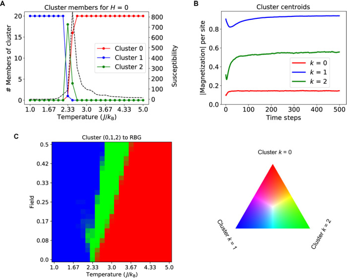
(A) Number of members of each cluster for applied field of H = 0 as a function of temperature. The clustering highlights that there is a marked change in the relaxation behavior across the phase transition temperature (~2.3). For comparison, the susceptibility is plotted as a dashed line, taken from the simulations in fig. S1, and good agreement is observed. k_B, Boltzmann constant. (B) Mean responses of each cluster (that is, the cluster centroids) are plotted. (C) Field-temperature phase diagram as mapped by clustering. The map shows the number of relaxation curves at each field and temperature belonging to the particular cluster 0, 1, and 2, that is, red, blue, and green, respectively. The triangle color map shows the number of labels (maximum value is 20; see fig. S1).

To explore this concept experimentally, we have chosen a ferroelectric relaxor system, (1 − x)Pb(Mg_1/3Nb_2/3)O₃ − xPbTiO₃ (PMN-xPT) as a model system. The system’s properties including the dielectric susceptibility, electromechanical coupling, and piezoelectric coefficient all peak at ~30% PT concentration, which is associated with a phase transition from a rhombohedral phase to a monoclinic phase at the morphotropic phase boundary (and eventually, at 35% PT, to a tetragonal phase) and which has been well explored with the Landau-Ginzburg and phase-field modeling in previous works (25, 26). The same phase transition can be accessed at lower levels of the PT content, if the sample is heated to slightly above room temperature or if sufficiently large fields are applied (27, 28). Thus, this system serves as a test case for whether the structural phase transition can be explored without having to directly map the structural order parameter, which is inaccessible by atomic force microscopy (AFM) measurements.

We use piezoresponse force microscopy (PFM), which measures the piezoresponse (strain) generated by applying an electric field from an AFM tip, in nanoscopic volumes. At the same time, given that the strain is related to the order parameter, but is not a direct probe, determining the phase transition temperature particularly in light of artifacts that are present in PFM measurements and the fact that both phases exhibit large piezoelectric response remains a challenge (29). We are able to successfully show that using machine learning on the collection of the relaxation curves in the broad temperature-bias parameter space allows automatic construction of a phase diagram similar to that of the bulk (30).

RESULTS

PFM measurements

We conduct PFM imaging on the PMN-27.5PT crystals. Details of the sample preparation can be found elsewhere (31). The crystals are polished, allowing the AFM measurements with minimal topographic cross-talk. Results of basic PFM imaging are shown in fig. S2 but demonstrate a flat surface with no distinguishable features in the piezoresponse maps. Given the absence of contrast, it is not possible to determine the structural phases that form during heating from these images.

To further explore this material in detail and to probe the dynamics experimentally, we use band excitation PFM (BE-PFM) (32). This is a method that adds to standard PFM imaging via the addition of a spectroscopy component (that allows measurement of the piezoresponse as a function of voltage and time) and a BE component. The BE component is used to detect the piezoresponse and improves single-frequency lock-in–based detection schemes by operating across a band of frequencies, centered on the resonant frequency of the cantilever, and thereby allowing signal amplification by the quality factor (typically by a factor of ~100). A BE wave packet is sent to the tip, and by measuring the cantilever response and subsequent Fourier transformation, a simple harmonic oscillator function can be fit to the real and imaginary components of the measured spectrum. This fitting enables extraction of the amplitude, phase, resonant frequency, and quality factor. The detection scheme is coupled with a triangular dc envelope as shown in Fig. 2A. The dc pulses excite the sample in the probed volume of the AFM tip, and the BE packet allows reading of the piezoresponse, including amplitude, phase, and frequency signals as a function of time (that is, the piezoelectric relaxation) immediately after the removal of dc voltage. The use of BE in this experiment enables enhanced quantitative measurement (due to greatly reduced topographic cross-talk), as well as better sensitivity to changes in piezoresponse, as we take advantage of the resonance. We obtained 12 relaxation curves at each spatial location, with the 12 curves associated with the varying amplitudes of dc pulses. In this manner, we build up a 4D data set of piezoresponse amplitude A as a function of position, bias, time, and temperature, that is, A = A(x, y, V, t, T). Here, x and y are spatial positions, V is the voltage applied to the tip (dc), t is the time after each dc pulse, and T is the temperature. Note that we performed the experiments over a 10 × 10 spectral grid of points to obtain good statistics.

Fig. 2. The BE-PFM waveform for piezoresponse relaxation measurements and the eigenvectors and eigenvalues of the SVD process.

(A) The waveform of the PFM spectroscopic experiment consists of a series of dc pulses of alternating polarity, with increasing amplitude of up to ±18 V. In between the dc pulses, the piezoresponse as a function of time is measured by applying a sequence of ac read voltage. (B) First six eigenvectors of piezoresponse relaxation in 0.2 s measured period. The first three eigenvectors show the main trends in relaxation behaviors of the amplitude signal. (C) Eigenvalues of the first four components as a function of temperatures and spatial coordinates. The eigenvalues of the first two components indicate a dramatic change at 80°C, which belongs to the M_B to M_C phase transition point (black dashed line) of this material.

Principal components analysis

For the initial analysis of the data set, we chose the 12th cycle, that is, V_dc = 18 V, as a representative for analysis. To determine the differences in relaxation behavior, we used principal components analysis (PCA), which is a basic machine learning method used for denoising, dimensionality reduction, and visualization of large multidimensional data sets (33). We perform PCA on the 2D data set A = A([x, y, T], t), where A is the amplitude signal from PFM, t is the time dimension, and T is the temperature dimension, using the singular value decomposition (SVD) method to obtain the eigenvectors and the eigenvalues. Here, we are concerned with determining the decomposition for the matrix M of size m × n

$$\mathit{M}=\mathit{U}\mathit{S}\mathit{V}*$$

where U is an m × m unitary matrix, S is a diagonal matrix of size m × n, and V* is an n × n unitary matrix. The eigenvectors (principal components) are given by the columns of V, and the columns of U and S are the scores (“loadings”) (assuming that the PCA is calculated from the covariance matrix, where the data are preprocessed by centering each column). It should be noted that we analyzed 100 curves (each consisting of a vector of length 28 time steps) at eight temperature steps, with a resultant matrix size of 800 × 28. The full results from the SVD are shown in Fig. 2 (B and C). Figure 2B illustrates the first six eigenvectors and indicates that the first and second components have stretched exponential features that are the basic tendency of each piezoresponse relaxation curve. Meanwhile, the third component has a rather large dip at around 50 ms. Finally, the components subsequent to the fifth component are near zero and contain little useful information, which is further supported by the scree plot in fig. S3. The first four eigenvalues (columns) at different temperatures (rows) are shown in Fig. 2C. Given that the measurement was 100 curves captured on a 10 × 10 spectroscopic grid of points, we plot the eigenvalues in the same manner, splitting them as a function of temperature. The first column shows the first eigenvalue component, and the values markedly decrease from 70° to 80°C, whereas the second eigenvalue changes simultaneously in this region increasing substantially. Theoretically, we expect that the material-specific responses (in this case, piezoelectric relaxation) should lie on the low-dimensional manifold in the response space of the system. Then, the phase boundaries are defined as regions where this response changes rapidly across this manifold. Thus, the sudden change in the eigenvalues for components 1 and 2 across a particular temperature range indicates the possibility that this stems from the phase transition (changes not related to phase transitions would manifest more gradually). Here, the critical point is related to the M_B to M_C phase transition in this material. Not all the components change across the phase transition. In the third and fourth columns, the eigenvalues seem to be more random, so there is no clear change after the third component. This suggests that some of the features of the relaxation are related to material or measurement parameters that are unchanged by the structural phase transition (possibly stemming from surface electrochemical effects). Additional details are provided in the Supplementary Materials.

Clustering approach

As shown earlier, the PCA is sufficient to determine the onset of the phase transition. However, the components are only statistically defined and do not have physical meaning per se. It also presents problems in the identification of phases, given that some are focused on more general (large-scale) features, whereas others are important to describe more fine-structure features that do not vary across the phase transition. To circumvent these issues, we explore whether basic clustering of the relaxation dynamics can fully map the temperature-bias phase diagram. In contrast to the PCA, where we considered only a small subset of the data here, we performed k-means clustering on the entire relaxation data for all (positive) voltage pulses at all temperatures. We posited the existence of three distinct regimes in the phase space (that is, three clusters), and each relaxation curve could be assigned as belonging to one of these three clusters. Figure 3A shows the means of the three clusters that were determined using this method. The first and second clusters show the exponential relaxation trend with varying offsets and decay times, whereas the third cluster indicates no relaxation. Because we measured 100 curves at each bias and temperature, we plot the results as a 2D plot on the temperature-bias axes, where the color scale represents the number of members within each cluster. The temperature-bias phase diagram representing the relaxation behaviors is built in Fig. 3B, with the results compressed by individual clusters. Figure 3B illustrates the ratio of three clusters (k = 0, 1, and 2) using the RGB scale as a function of bias and temperature. The original data (see the Supplementary Materials) with a maximum value of 100 are normalized to the RGB color triangle as shown in Fig. 1C. Red, blue, and green belong to cluster labels k = 0, 1, and 2, respectively. Apparently, relaxation curves belonging to the k = 0 cluster appear only at high temperature, as indicated by the larger number of members for those conditions. Similarly, the second cluster (k = 1) corresponds to the lower-temperature or low-voltage values at high temperature. The M_B to M_C phase regions in the temperature–dc bias phase diagram is determined and marked by the dashed profiles. Finally, the third cluster appears to be dominated by curves not exhibiting relaxation that mostly appear at low-voltage values and are absent at higher voltages. This suggests that some perturbation (threshold field) is required at these temperatures to initiate the structural phase transition.

Fig. 3. K-means clustering on the amplitude data sets A = A (V, T, t), where V is the bias voltage, T is the temperature, and t is the relaxation time.

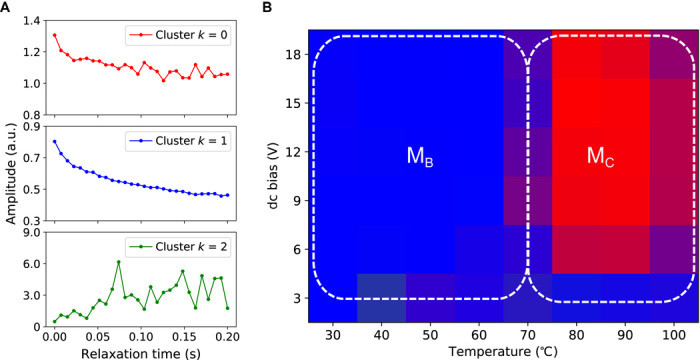
(A) Cluster centers of k-means clustering. (B) The corresponding labels of k-means clustering indicate the M_B to M_C phase transition boundary in the field-temperature phase diagram. The colors representing the number of labels with a maximum value of 100 is normalized to the RGB color triangle in Fig. 1C. Red, blue, and green belong to cluster labels, that is, k = 0, 1, and 2, respectively. a.u., arbitrary units.

DISCUSSION

These results show the ability to determine the phase diagram of this system without a priori knowledge of the mechanisms at play and using only local information that are proxies to the dynamics of the hidden structural phases through which the system transitions. We have previously argued for the possibility of the field-induced phase transition in these systems, which is supported by analytical theory, phase-field modeling, and acoustic measurements (34). Here, we investigate the relaxation response as a function of temperature and fully delineate the temperature-bias phase diagram. It should be noted that apart from the effect at low bias (not enough relaxation observed), there does not appear to be substantial dependence of the phase transition temperature on the applied bias. This may be due to the coarseness of our temperature control in the AFM, but even at this resolution, some insight is gained. For example, in Fig. 3B, the number of members of cluster 2 (k = 1) at 80°C for 6 V appears to be 24, but at 9 V, this has changed to 6, indicating a complete crossover to the M_C phase at higher fields. We further observe some elastic softening related to the structural phase transition at higher temperatures (see the Supplementary Materials). Furthermore, analysis of the relaxation data using functional fitting procedures was also undertaken (see the Supplementary Materials). We conclude that although it is possible to infer the presence of the phase transition using this method, the small variations observed in the experiment and the large dispersions in measured values make accurate determinations difficult and are inferior to the clustering or PCA-based methods.

This work provides a clear demonstration of the use of unsupervised machine learning on raw experimental data for automatic determination of phase diagrams on a system where identification of underpinning physical mechanisms is generally impossible and microscopic degrees of freedom are unavailable for observations. Despite this, the clustering of relaxation dynamics into distinct phases, as a function of local (field) and global (temperature) parameters, not only is possible but also is shown to be superior to the traditional methods of functional fitting and observation of distinct relaxation times. This is understandable, because the relaxation dynamics in ferroelectric relaxors, especially when measured by PFM, can be remarkably complex (35), and the manifestation of the different structural phases in modulating the relaxation time is not likely to be trivial. However, their influence will certainly be present on the shape of the resulting curves.

The approach shown here is general and could be used to explore complex phase diagrams measured in nanoscale volumes, and also represents a new approach to mine experimental data as a function of applied stresses. For instance, it could be used to explore a variety of field and pressure-induced transitions, including transitions in superionic materials or needle domains (for avalanches and jamming transitions) (36).

MATERIALS AND METHODS

The single crystals of (1 − x)Pb(Mg_1/3Nb_2/3)O₃ – xPbTiO₃ were grown from high-temperature solution according to the method described elsewhere (31). The (001)-oriented sample for PFM imaging and measurements was glued onto a conductive sample plate with silver epoxy, which served as the bottom electrode and grounded during all PFM measurements. The temperature-dependent PFM measurements were conducted in a built-in temperature-controlled chamber with Budget Sensors cantilevers (k ~1 N/m) and a free resonance of ~75 kHz in air on a Cypher ES AFM platform from Asylum Research. Two National Instruments PXI-based cards were set for the dc plus ac relaxation signal generation and data acquisition for the BE relaxation experiments, which were performed using in-house scripts written in LabVIEW v11 and MATLAB v2011. All data analyses were carried out using Python 2.7.

SUPPLEMENTARY MATERIALS

Supplementary material for this article is available at http://advances.sciencemag.org/cgi/content/full/4/3/eaap8672/DC1

fig. S1.1. Results of 2D Ising simulation.

fig. S1.2. The field-temperature phase diagram as mapped by clustering.

fig. S2. PFM images of the PMN-PT single crystal.

fig. S3. The scree plot in the SVD process.

fig. S4. Statistical analysis with functional fitting.

fig. S5. The mean values of the first two components of eigenvalues and temperature-dependent relaxation curves.

fig. S6. The KWW fitting parameters with temperature and dc bias dependence.

fig. S7. The labels of k-means clustering.

References (37–40)

REFERENCES AND NOTES

- 1.Bernevig B. A., Hughes T. L., Zhang S.-C., Quantum spin Hall effect and topological phase transition in HgTe quantum wells. Science 314, 1757–1761 (2006). [DOI] [PubMed] [Google Scholar]
- 2.Ahn K. H., Lookman T., Bishop A. R., Strain-induced metal-insulator phase coexistence in perovskite manganites. Nature 428, 401–404 (2004). [DOI] [PubMed] [Google Scholar]
- 3.Kusne A. G., Gao T., Mehta A., Ke L., Nguyen M. C., Ho K.-M., Antropov V., Wang C.-Z., Kramer M. J., Long C., Takeuchi I., On-the-fly machine-learning for high-throughput experiments: Search for rare-earth-free permanent magnets. Sci. Rep. 4, 6367 (2014). [DOI] [PMC free article] [PubMed] [Google Scholar]
- 4.Al-Barakaty A., Prosandeev S., Wang D., Dkhil B., Bellaiche L., Finite-temperature properties of the relaxor PbMg1/3Nb2/3O3 from atomistic simulations. Phys. Rev. B 91, 214117 (2015). [Google Scholar]
- 5.Ahart M., Somayazulu M., Cohen R. E., Ganesh P., Dera P., Mao H.-k., Hemley R. J., Ren Y., Liermann P., Wu Z., Origin of morphotropic phase boundaries in ferroelectrics. Nature 451, 545–548 (2008). [DOI] [PubMed] [Google Scholar]
- 6.Horiuchi S., Tokunaga Y., Giovannetti G., Picozzi S., Itoh H., Shimano R., Kumai R., Tokura Y., Above-room-temperature ferroelectricity in a single-component molecular crystal. Nature 463, 789–792 (2010). [DOI] [PubMed] [Google Scholar]
- 7.Sherman D., Pracht U. S., Gorshunov B., Poran S., Jesudasan J., Chand M., Raychaudhuri P., Swanson M., Trivedi N., Auerbach A., Scheffler M., Frydman A., Dressel M., The Higgs mode in disordered superconductors close to a quantum phase transition. Nat. Phys. 11, 188–192 (2015). [Google Scholar]
- 8.Otsuka K., Ren X., Physical metallurgy of Ti–Ni-based shape memory alloys. Prog. Mater. Sci. 50, 511–678 (2005). [Google Scholar]
- 9.Kivelson S. A., Fradkin E., Emery V. J., Electronic liquid-crystal phases of a doped Mott insulator. Nature 393, 550–553 (1998). [Google Scholar]
- 10.Takenaka H., Grinberg I., Liu S., Rappe A. M., Slush-like polar structures in single-crystal relaxors. Nature 546, 391–395 (2017). [DOI] [PubMed] [Google Scholar]
- 11.Wang D., Bokov A. A., Ye Z.-G., Hlinka J., Bellaiche L., Subterahertz dielectric relaxation in lead-free Ba(Zr,Ti)O3 relaxor ferroelectrics. Nat. Commun. 7, 11014 (2016). [DOI] [PMC free article] [PubMed] [Google Scholar]
- 12.Balashova E. V., Lemanov V. V., Tagantsev A. K., Sherman A. B., Shomuradov Sh. H., Betaine arsenate as a system with two instabilities. Phys. Rev. B 51, 8747–8752 (1995). [DOI] [PubMed] [Google Scholar]
- 13.Balashova E. V., Tagantsev A. K., Polarization response of crystals with structural and ferroelectric instabilities. Phys. Rev. B 48, 9979–9986 (1993). [DOI] [PubMed] [Google Scholar]
- 14.Tanaka A., Tomiya A., Detection of phase transition via convolutional neural networks. J. Phys. Soc. Jpn. 86, 063001 (2017). [Google Scholar]
- 15.van Nieuwenburg E. P. L., Liu Y.-H., Huber S. D., Learning phase transitions by confusion. Nat. Phys. 13, 435–439 (2017). [Google Scholar]
- 16.V. Stanev, C. Oses, A. G. Kusne, E. Rodriguez, J. Paglione, S. Curtarolo, I. Takeuchi, Machine learning modeling of superconducting critical temperature. https://arxiv.org/abs/1709.02727 (2017).
- 17.Zdeborová L., Machine learning: New tool in the box. Nat. Phys. 13, 420–421 (2017). [Google Scholar]
- 18.Machta B. B., Chachra R., Transtrum M. K., Sethna J. P., Parameter space compression underlies emergent theories and predictive models. Science 342, 604–607 (2013). [DOI] [PubMed] [Google Scholar]
- 19.Wang J., Paesani S., Santagati R., Knauer S., Gentile A. A., Wiebe N., Petruzzella M., O’Brien J. L., Rarity J. G., Laing A., Thompson M. G., Experimental quantum Hamiltonian learning. Nat. Phys. 13, 551–555 (2017). [Google Scholar]
- 20.Bokov A. A., Ye Z.-G., Recent progress in relaxor ferroelectrics with perovskite structure. J. Mater. Sci. 41, 31–52 (2006). [Google Scholar]
- 21.Li B., Zhou D., Han Y., Assembly and phase transitions of colloidal crystals. Nat. Rev. Mater. 1, 15011 (2016). [Google Scholar]
- 22.Salje E. K. H., Ding X., Zhao Z., Lookman T., Saxena A., Thermally activated avalanches: Jamming and the progression of needle domains. Phys. Rev. B 83, 104109 (2011). [Google Scholar]
- 23.Schoenholz S. S., Cubuk E. D., Sussman D. M., Kaxiras E., Liu A. J., A structural approach to relaxation in glassy liquids. Nat. Phys. 12, 469–471 (2016). [Google Scholar]
- 24.J. MacQueen, Some methods for classification and analysis of multivariate observations, in Proceedings of the Fifth Berkeley Symposium on Mathematical Statistics and Probability, Volume 1: Statistics (University of California Press, 1967), pp. 281–297. [Google Scholar]
- 25.Zhao X., Fang B., Cao H., Guo Y., Luo H., Dielectric and piezoelectric performance of PMN–PT single crystals with compositions around the MPB: Influence of composition, poling field and crystal orientation. Mater. Sci. Eng. B 96, 254–262 (2002). [Google Scholar]
- 26.A.-B. M. A. Ibrahim, R. Murgan, M. K. A. Rahman, J. Osman, Morphotropic phase boundary in ferroelectric materials, in Ferroelectrics—Physical Effects, M. Lallart, Ed. (InTech, 2011), pp. 3–26. [Google Scholar]
- 27.Tu C.-S., Hsieh C.-M., Chien R. R., Schmidt V. H., Wang F.-T., Chang W. S., Nanotwins and phases in high-strain Pb(Mg1/3Nb2/3)1-xTixO3 crystal. J. Appl. Phys. 103, 074117 (2008). [Google Scholar]
- 28.Tu C.-S., Chien R. R., Wang F.-T., Schmidt V.-H., Han P., Phase stability after an electric-field poling in Pb(Mg1/3Nb2/3)1-xTixO3 crystals. Phys. Rev. B 70, 220103 (2004). [Google Scholar]
- 29.Jesse S., Vasudevan R. K., Collins L., Strelcov E., Okatan M. B., Belianinov A., Baddorf A. P., Proksch R., Kalinin S. V., Band excitation in scanning probe microscopy: Recognition and functional imaging. Annu. Rev. Phys. Chem. 65, 519–536 (2014). [DOI] [PubMed] [Google Scholar]
- 30.Słodczyk A., Kania A., Daniel Ph., Structural, dielectric and Raman scattering studies of (1- x)PbMg1/3Nb2/3O3– xPbTiO3 single crystals (0≤ x ≤ 0.38). Phase Transit. 79, 399–413 (2006). [Google Scholar]
- 31.Dong M., Ye Z.-G., High-temperature solution growth and characterization of the piezo-/ferroelectric (1−x)Pb(Mg1/3Nb2/3)O3–xPbTiO3 [PMNT] single crystals. J. Cryst. Growth 209, 81–90 (2000). [Google Scholar]
- 32.Vasudevan R. K., Jesse S., Kim Y., Kumar A., Kalinin S. V., Spectroscopic imaging in piezoresponse force microscopy : New opportunities for studying polarization dynamics in ferroelectrics and multiferroics. MRS Commun. 2, 61–73 (2012). [Google Scholar]
- 33.Jesse S., Kalinin S. V, Principal component and spatial correlation analysis of spectroscopic-imaging data in scanning probe microscopy. Nanotechnology 20, 85714 (2009). [DOI] [PubMed] [Google Scholar]
- 34.Vasudevan R. K., Khassaf H., Cao Y., Zhang S., Tselev A., Carmichael B., Okatan M. B., Jesse S., Chen L.-Q., Alpay S. P., Kalinin S. V., Bassiri-Gharb N., Acoustic detection of phase transitions at the nanoscale. Adv. Funct. Mater. 26, 478–486 (2016). [Google Scholar]
- 35.Kalinin S. V., Bonnell D. A., Imaging mechanism of piezoresponse force microscopy of ferroelectric surfaces. Phys. Rev. B 65, 125408 (2002). [Google Scholar]
- 36.Zapperi S., Cizeau P., Durin G., Stanley H. E., Dynamics of a ferromagnetic domain wall: Avalanches, depinning transition, and the Barkhausen effect. Phys. Rev. B 58, 6353–6366 (1998). [Google Scholar]
- 37.Ren X., Large electric-field-induced strain in ferroelectric crystals by point-defect-mediated reversible domain switching. Nat. Mater. 3, 91–94 (2004). [DOI] [PubMed] [Google Scholar]
- 38.Li Y.-J., Wang J.-J., Ye J.-C., Ke X.-X., Gou G.-Y., Wei Y., Xue F., Wang J., Wang C.-S., Peng R.-C., Deng X.-L., Yang Y., Ren X.-B., Chen L.-Q., Nan C.-W., Zhang J.-X., Mechanical switching of nanoscale multiferroic phase boundaries. Adv. Funct. Mater. 25, 3405–3413 (2015). [Google Scholar]
- 39.Li Q., Cao Y., Yu P., Vasudevan R. K., Laanait N., Tselev A., Xue F., Chen L. Q., Maksymovych P., Kalinin S. V., Balke N., Giant elastic tunability in strained BiFeO3 near an electrically induced phase transition. Nat. Commun. 6, 8985 (2015). [DOI] [PMC free article] [PubMed] [Google Scholar]
- 40.Heo Y., Jang B.-K., Kim S. J., Yang C.-H., Seidel J., Nanoscale mechanical softening of morphotropic BiFeO3. Adv. Mater. 26, 7568–7572 (2014). [DOI] [PubMed] [Google Scholar]
Associated Data
This section collects any data citations, data availability statements, or supplementary materials included in this article.