Radiomics analysis of pulmonary nodules in low‐dose CT for early detection of lung cancer

Abstract

Purpose

To develop a radiomics prediction model to improve pulmonary nodule (PN) classification in low‐dose CT. To compare the model with the American College of Radiology (ACR) Lung CT Screening Reporting and Data System (Lung‐RADS) for early detection of lung cancer.

Methods

We examined a set of 72 PNs (31 benign and 41 malignant) from the Lung Image Database Consortium image collection (LIDC‐IDRI). One hundred three CT radiomic features were extracted from each PN. Before the model building process, distinctive features were identified using a hierarchical clustering method. We then constructed a prediction model by using a support vector machine (SVM) classifier coupled with a least absolute shrinkage and selection operator (LASSO). A tenfold cross‐validation (CV) was repeated ten times (10 × 10‐fold CV) to evaluate the accuracy of the SVM‐LASSO model. Finally, the best model from the 10 × 10‐fold CV was further evaluated using 20 × 5‐ and 50 × 2‐fold CVs.

Results

The best SVM‐LASSO model consisted of only two features: the bounding box anterior–posterior dimension (BB_AP) and the standard deviation of inverse difference moment (SD_IDM). The BB_AP measured the extension of a PN in the anterior–posterior direction and was highly correlated (r = 0.94) with the PN size. The SD_IDM was a texture feature that measured the directional variation of the local homogeneity feature IDM. Univariate analysis showed that both features were statistically significant and discriminative (P = 0.00013 and 0.000038, respectively). PNs with larger BB_AP or smaller SD_IDM were more likely malignant. The 10 × 10‐fold CV of the best SVM model using the two features achieved an accuracy of 84.6% and 0.89 AUC. By comparison, Lung‐RADS achieved an accuracy of 72.2% and 0.77 AUC using four features (size, type, calcification, and spiculation). The prediction improvement of SVM‐LASSO comparing to Lung‐RADS was statistically significant (McNemar's test P = 0.026). Lung‐RADS misclassified 19 cases because it was mainly based on PN size, whereas the SVM‐LASSO model correctly classified 10 of these cases by combining a size (BB_AP) feature and a texture (SD_IDM) feature. The performance of the SVM‐LASSO model was stable when leaving more patients out with five‐ and twofold CVs (accuracy 84.1% and 81.6%, respectively).

Conclusion

We developed an SVM‐LASSO model to predict malignancy of PNs with two CT radiomic features. We demonstrated that the model achieved an accuracy of 84.6%, which was 12.4% higher than Lung‐RADS.

1. Introduction

Lung cancer is the leading cause of cancer death in the world. The National Lung Cancer Screening Trial (NLST) showed a clear survival benefit for screening with a low‐dose computed tomography (LDCT) in current and former smokers.¹ The early detection of lung cancer by LDCT can reduce mortality. Recently, the Lung Imaging Reporting and Data System (Lung‐RADS) was developed by the American College of Radiology (ACR) to standardize the screening of lung cancer on CT images.^{2, 3} However, LDCT dramatically increases the number of indeterminate pulmonary nodules (PNs) and produces a high false‐positive diagnostic rate, which leads to overdiagnosis.⁴ Therefore, it is important to develop new approaches to improve accuracy.

Computer‐aided detection/diagnosis (CAD; specifically, CADe for detection and CADx for diagnosis) systems have been investigated to detect PNs and classify malignant and benign PNs.^{5, 6, 7, 8, 9, 10} In the mid‐90s, Gurney and Swensen conducted a PN characterization study with an artificial neural network (ANN) and features that were subjectively assessed by radiologists.¹¹ Kawata et al. proposed quantitative surface characterization to classify malignant and benign PNs.¹² McNitt‐Gray et al. proposed a pattern classification approach to characterize PNs, which used quantitative features including attenuation (intensity), size, shape, and texture.¹³ Aoyama et al. proposed an automatic scheme which segment PNs using dynamic programming technique and determine malignant PNs using linear discriminant analysis (LDA) classification.¹⁴ Armato et al. developed a serial approach PN classification following automatic PN detection.¹⁵ A rule‐based scheme was applied to reduce PN candidates in the detection, and two LDA classifiers were applied for the detection and the classification of PNs. Shah et al. investigated the utility of a CAD system using volumetric and contrast enhancement features.¹⁶ Suzuki et al. developed the massive training ANN to filter out benign appearances in CT image.¹⁷ Way et al. developed an automatic 3D active contour segmentation method and extracted surface features from the segmented PNs.^{18, 19} Lee et al. developed ensemble classifications using random subspace method or genetic algorithm feature selection with LDA classifier.²⁰ Han et al. investigated texture feature analysis to differentiate malignant and benign PNs.²¹ The early successes of the CAD systems illustrated that quantitative medical image analysis has the potential to improve the performance of detecting cancer on chest CT.

Recently, radiomics studies, which extract a large number of quantitative features from medical images and subsequently perform data mining, have been proposed for various clinic applications.^{22, 23, 24, 25, 26} For instance, radiomics has been studied for the prediction of tumor responses and patient outcomes, resulting in more accurate prediction of local control and overall survival.^{22, 23, 24, 26, 27, 28, 29} Lung cancer screening using radiomics has also been studied.^{30, 31, 32, 33} Hawkins et al. proposed a random forest classifier³⁰ using 23 stable radiomic features.^{34, 35} Ma et al. proposed a random forest classifier using 583 radiomic features.³¹ Buty et al. developed a random forest classifier using 4096 appearance features extracted with a pretrained deep neural network and 400 shape features extracted with spherical harmonics.³² Kumar et al. developed a deep neural network model using 5000 features.³³ Liu et al. proposed a linear classifier based on 24 image traits visually scored by physicians.^{36 .}

Despite the improved prediction accuracy reported in these radiomics studies, there are limitations including the possibility of overfitting the model to the data and lack of clinical/biological interpretations of the intimidatingly large number of radiomic features. To overcome these limitations, we first identified distinctive radiomic features using hierarchical clustering and then constructed a support vector machine (SVM) model with only two important features chosen by a least absolute shrinkage and selection operator (LASSO). We compared the performance of this model and Lung‐RADS on a public database.

2. Materials and methods

2.A. Dataset and Lung‐RADS

The Lung Image Database Consortium image collection (LIDC‐IDRI) in The Cancer Imaging Archive (TCIA) contains 1018 cases with low‐dose screening thoracic CT scans and marked‐up annotated lesions.³⁷ Four experienced thoracic radiologists performed contouring and image annotation. A subset of cases (n = 157) has associated diagnostic data regarding the screening CT scans. Of these 157 patients, 36 had benign lesions, 43 had malignant primary lung cancers, and the remainders were unknown or had metastatic tumors. Forty‐two malignant lung cancer cases and six benign cases were diagnosed by biopsy or surgical resection, and 18 benign diseases were determined by stability at 2‐year follow‐up. Lastly, four cases (one malignant and three benign cases) were determined by lesional progression or response. However, five benign cases and two malignant cases had missing PN contours. Thus, we evaluated 72 cases (31 benign and 41 malignant cases) who had both diagnostic data and PN contours. Each evaluated PN had at least one to four contours delineated by the four radiologists. Figure 1 shows distributions of size, type, calcification, and spiculation of PNs in the dataset.

Figure 1.

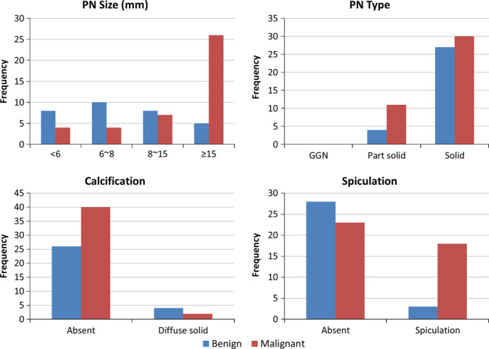
Distributions of pulmonary nodule size, type, calcification, and spiculation in the dataset. [Color figure can be viewed at wileyonlinelibrary.com]

The tube peak potential energy used for most scan acquisition was 120 kV (n = 71) and only one scan was 140 kV. Tube current ranged from 80 to 570 mA (mean: 322.5 mA). Slice thicknesses were 1.0 mm (n = 5), 1.25 mm (n = 13), 1.5 mm (n = 1), 2.0 mm (n = 11), and 2.5 mm (n = 42). Reconstruction interval ranged from 0.625 to 2.5 mm (mean: 1.80 mm). The in‐plane pixel size ranged from 0.547 to 0.898 mm (mean: 0.721 mm). Each axial slide of CT scan was 512 × 512 pixels. While the convolution kernels used for image reconstruction differ among manufacturers, these convolution kernels may be classified broadly as “standard/nonenhancing” (n = 43), “slightly enhancing” (n = 17), and “over enhancing” (n = 12) (in order of increasing spatial frequencies accentuated by each class). Forty‐four scans were contrast‐enhanced CT.

We performed Lung‐RADS categorization based on the PN contour and annotations made by the four radiologists in the LIDC‐IDRI dataset.² A study radiologist (CL) reviewed the categorization results. As shown in Table 1, the Lung‐RADS categorization is mainly based on PN size (the average of the longest and shortest diameters on axial slice) with some consideration to calcification, PN type (solid, part‐solid, and nonsolid or ground glass nodule/GGN), and additional suspicious features. To match the original LIDC‐IDRI diagnosis, categories 3 and lower PNs are deemed as benign and category 4 (4A, 4B, and 4X) PNs as malignant.

Table 1.

Summary of Lung‐RADS categorization for baseline screening

Category	Baseline screening	Malignancy
1	No PNs; PNs with calcification	Negative <1% chance of malignancy
2	Solid/part‐solid: <6 mm GGN: <20 mm	Benign appearance <1% chance of malignancy
3	Solid: ≥6 to <8 mm Part‐solid: ≥6 mm with solid component <6 mm GGN: ≥20 mm	Probably benign 1–2% chance of malignancy
4A	Solid: ≥8 to <15 mm Part‐solid: ≥8 mm with solid component ≥6 and <8 mm	Suspicious 5–15% chance of malignancy
4B	Solid: ≥15 mm Part‐solid: Solid component ≥8 mm	>15% chance of malignancy
4X	Category 3 or 4 PNs with suspicious features (e.g., enlarged lymph nodes) or suspicious imaging findings (e.g., spiculation)	>15% chance of malignancy

2.B. Radiomic features

Figure 2 shows the flowchart for the extraction of radiomic features and the construction of a prediction model. To extract radiomic features from a CT, we built the following image analysis pipeline using the Insight Segmentation and Registration Toolkit (ITK, National Library of Medicine; Bethesda, MD).³⁸ First, we re‐sampled the CT images to make voxels isotropic (1 mm). Second, we generated a consensus contour for each PN with 2 or more contours by using the simultaneous truth and performance level estimation (STAPLE).^{39, 40} Third, we extracted 103 radiomic features from each PN to quantify its intensity, shape, and texture (spatial variations).^{23, 27, 41} Finally, we performed a univariate analysis using Wilcoxon rank‐sum test and the area under the receiver operating characteristic curve (AUC) to evaluate the significance of each feature. P‐values were adjusted using Bonferroni correction because we tested multiple features (n = 103) for a single outcome.⁴²

Figure 2.

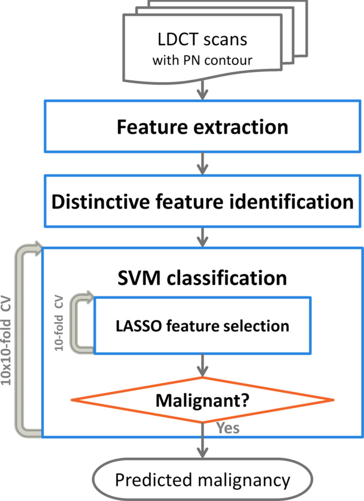
A flowchart of the extraction of radiomic features and the construction of a prediction model. [Color figure can be viewed at wileyonlinelibrary.com]

Three types of radiomic features were extracted for each PN. Intensity features are first‐order statistical measures that quantify the level and distribution of CT attenuations in a PN. Shape features describe geometric characteristics (e.g., volume, diameter, elongation, and flatness) of a PN. CT texture features quantify the spatial patterns of tissue density, such as homogeneity, coarseness, and correlation of CT intensity in a PN by using Gray‐level co‐occurrence matrix (GLCM)⁴³ and gray‐level run‐length matrix (GLRM).^{44, 45} For texture features, the CT intensity was first normalized to the range of contrast stretching to simplify the spatial complexity due to a wide dynamic range of CT attenuation. The texture features were then computed on the GLCM and GLRM of the normalized volumes. The average value of each texture feature was computed over all 13 directions to obtain rotationally invariant features. Furthermore, the length of runs was normalized by the diagonal length of the PN's bounding box to make the GLRM scale invariant.

2.C. Prediction model

Before constructing a prediction model, we identified distinctive radiomic features using Ward's hierarchical clustering method,⁴⁶ which maximized the total within‐cluster (Pearson) correlation (r). Each feature started in its cluster. Pairs of clusters were merged if the total within‐cluster correlation was larger after merging than before merging, as one moved up the hierarchy. This resulted in a hierarchical feature cluster tree. The tree was then divided into several prominent clusters (feature groups) by cutting using a threshold r ≥ 0.85. If a feature was the representative feature of a feature group, which had the smallest within‐cluster correlation, or if a feature was independent to all other features, it was identified as a distinctive feature. Other features were redundant and were removed from subsequent analysis.

An SVM classifier was, then, constructed for the prediction of PN malignancy coupled with a LASSO feature selection. All distinctive features were fed to the SVM classifier in a manner of a tenfold cross‐validation (CV). Within each fold CV of the model building process, LASSO was applied to select the ten most important distinctive features by using another (inner loop) tenfold CV. An SVM classifier was then constructed to predict PN malignancy. A radial basis kernel function was employed in the SVM classifier, with its parameters experimentally chosen: γ = 0.001 and C = 64. We repeated the outer‐loop tenfold CV ten times to obtain the model accuracy (10 × 10‐fold CV). In each repetition, all patients were randomly partitioned into a training set (90% patients) and a testing set (10% patients). Finally, the stability of the best model from the 10 × 10‐fold CV was evaluated using 20 × 5‐ and 50 × 2‐fold CVs, in which 20% and 50% patients were partitioned into the testing set, respectively.²⁸ McNemar's test was used to compare prediction performance between the proposed radiomics model and Lung‐RADS.

3. Results

The hierarchical clustering identified 44 distinctive features from the total of 103 radiomic features. Among the 44 distinctive features, 14 were significant in univariate analysis (P < 0.05 after Bonferroni correction). These included four shape, eight texture, and two shape + intensity (intensity weighted shape features using image moments) features (Table S1).

Figure 3 shows that the model achieved the highest accuracy when two features were selected into the SVM classifier. The two most frequently selected features were (a) the PN bounding box (BB) anterior–posterior (AP) dimension (BB_AP), and (b) the standard deviation (SD) of inverse difference moment (SD_IDM, a texture feature that measures the directional variation of the local homogeneity feature IDM,⁴³ see Section 4.A). BB_AP and SD_IDM were selected as the first feature 57 times and 43 times, respectively. They were selected as the second feature 43 times and 57 times, respectively. Therefore, the two features were always selected into the best SVM classifier. The best single‐feature model achieved 75.1 ± 6.0% accuracy (0.75 ± 0.04 AUC). When adding the second feature in the model, the prediction accuracy was improved to 84.6 ± 1.5% (0.89 ± 0.01 AUC). However, the performance was worse when adding more than two features as shown in Fig. 3.

Figure 3.

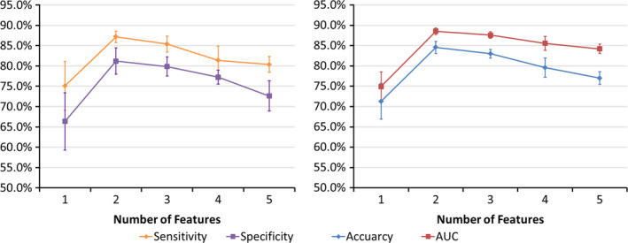
Performance of the prediction model with increasing number of features in the CV. [Color figure can be viewed at wileyonlinelibrary.com]

Figure 4 shows the difference between benign and malignant PNs for the two features and the PN size. As expected, the BB_AP was highly correlated with the PN size (r = 0.94), and the larger the BB_AP, the more likely a PN was malignant. The AP or left–right (LR) dimensions might be a better predictor than the superior–inferior (SI) dimension because of the typically higher axial resolutions (≤1 mm) than the longitudinal resolution (2–3 mm) in CT. The SD_IDM is a texture feature that measures the directional variation of the local homogeneity feature IDM. The smaller the SD_IDM, the more likely a PN was malignant.

Figure 4.

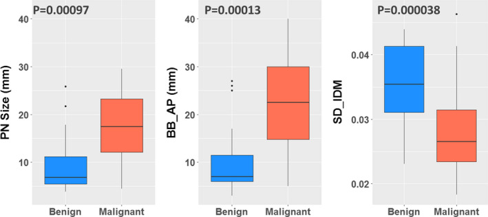
The box plots show the difference between benign and malignant for PN size and the selected features (BB_AP and SD_IDM). The Wilcoxon rank‐sum test obtained P‐values. [Color figure can be viewed at wileyonlinelibrary.com]

Table 2 compares the prediction performance of Lung‐RADS and the SVM‐LASSO model in 10 × 10‐fold CV. Figure 5 shows their ROC curves. The ROC curve for Lung‐RADS was generated by using each category as a cutoff for malignancy classification. The ROC curve for the SVM‐LASSO model was generated by computing the probability of nodule malignancy using the improved Platt's method.⁴⁷ The Lung‐RADS achieved an accuracy of 72.2% with four features (size, type, calcification, and suspicious features or image findings). The SVM‐LASSO model achieved an accuracy of 84.6% with two features (BB_AP and SD_IDM), which represented a 12.4% improvement over the Lung‐RADS. The performance difference was statistically significant (P = 0.026).

Table 2.

Prediction performance of Lung‐RADS and the SVM‐LASSO model

Prediction model	Sensitivity	Specificity	Accuracy	AUC	No. of features
Lung‐RADS	80.5%	61.3%	72.2%	0.77	4
SVM‐LASSO	87.2 ± 1.4%	81.2 ± 3.2%	84.6 ± 1.5%	0.89 ± 0.01	2

Figure 5.

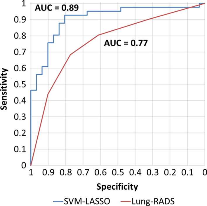
ROC curve analysis on the best model of SVM‐LASSO and Lung‐RADS for predicting malignant PNs. [Color figure can be viewed at wileyonlinelibrary.com]

Figure 6 shows a scatter plot of the two features and the classification curve by the SVM‐LASSO model. All five malignant PNs in the elliptical region a (red) were misclassified as benign by Lung‐RADS since they were small (size < 8 mm). Two example cases (c) and (d) were shown in Fig. 7. Note that case (c) was part‐solid with a solid component of 4 mm, and was thus classified as Category 3. On the other hand, all seven benign PNs in the elliptical region b (green) were misclassified as malignant by Lung‐RADS since they were large (size ≥ 8 mm). Two example cases (a) and (b) were shown in Fig. 7. The SVM‐LASSO model correctly classified these 12 PNs in both regions a and b by combining a size feature (BB_AP) and a texture feature (SD_IDM). There was one malignant case that was correctly classified by Lung‐RADS but misclassified by the SVM‐LASSO model. This case was indicated by arrow c in Fig. 6 and shown as the case (e) in Fig. 7. This PN was correctly classified by Lung‐RADS as malignant (category 4B) based on its size. Finally, nine cases were misclassified by both Lung‐RADS and the SVM‐LASSO model. Overall, the SVM‐LASSO model showed a clear advantage over Lung‐RADS. Figure 8 shows Lung‐RADS categorization on the scatter plots for solid and part‐solid PNs, respectively.

Figure 6.

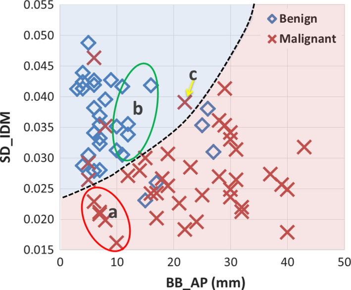
Scatter plot of the two important features and the classification curve (dashed line) by the SVM‐LASSO model for all PNs. [Color figure can be viewed at wileyonlinelibrary.com]

Figure 7.

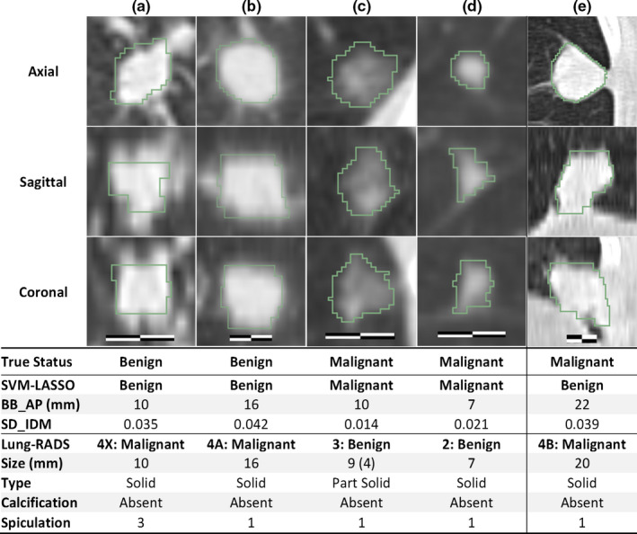
Cases misclassified by Lung‐RADS but correctly classified by the SVM‐LASSO model (a–d). A case correctly classified by Lung‐RADS but misclassified by the SVM‐LASSO model (e). The scale bar indicates 10 mm, window/level: 1400/−500 HU. The value in the parenthesis for size is the diameter of the solid component of a part‐solid PN. Spiculation is on a 1(no) to 5(marked) scale. [Color figure can be viewed at wileyonlinelibrary.com]

Figure 8.

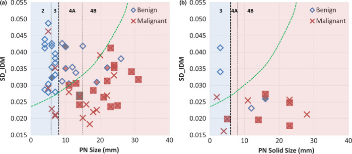
Lung‐RADS categorization on scatter plots for solid PNs (a) and part‐solid PNs (b). The SVM‐LASSO classification curve is approximately mapped on the plots (green dashed line). Lung‐RADS categorization is shown on top with black vertical dashed lines (the bold line indicates classification between benign and suspicious); PNs with calcification (category 1) are filled with dark gray, and PNs with spiculation (category 4X) are filled with light gray (red color online version). [Color figure can be viewed at wileyonlinelibrary.com]

The performance of the SVM‐LASSO model was stable when more patients were partitioned into the testing set with five‐ and twofold CVs compared with tenfold CV (Table 3). Only a small reduction in each accuracy measurement was observed, and even the accuracy of twofold CV (50% patients in the training set and 50% in the testing set) was 6.3% higher than that of the Lung‐RADS.

Table 3.

Prediction performance of the SVM‐LASSO using two features BB_AP and SD_IDM on 10 × 10‐, 20 × 5‐, and 50 × 2‐fold CVs

	Sensitivity	Specificity	Accuracy	AUC
10 × 10‐fold	87.2 ± 1.4%	81.2 ± 3.2%	84.6 ± 1.5%	0.89 ± 0.01
20 × 5‐fold	86.5 ± 2.5%	80.9 ± 2.9%	84.1 ± 2.0%	0.88 ± 0.02
50 × 2‐fold	85.7 ± 4.5%	76.1 ± 10.6%	81.6 ± 5.7%	0.87 ± 0.04

4. Discussion

We demonstrated that the SVM‐LASSO model achieved 84.6% accuracy, which was 12.4% higher than that of the Lung‐RADS. Accurate diagnosis of malignant PNs on LDCT screening is critical because LDCT dramatically increases the number of indeterminate PNs, leading to overdiagnosis.⁴ This model has the potential to spare individuals with benign growths from the biopsies and 2‐year multiple follow‐up examinations while allowing effective treatments to be immediately initiated for lung cancer.

4.A. SD_IDM feature

IDM is a texture feature that measures the local homogeneity.⁴³ The SD_IDM measures the directional variation of the IDM in 13 directions. As shown in Figs. 9 and 10, benign PNs appeared to be more homogeneous with generally higher IDMs in each direction as well as in the Mean_IDM (average of IDMs in all 13 directions) than malignant PNs of similar size. More importantly, benign PNs tended to be more homogeneous with much higher IDMs in AP and/or SI directions than in the other 12 or 11 directions. This led to a larger directional variation of the IDM or higher SD_IDM for benign PNs. The SD_IDM was even higher (≥0.041) for all four cases with diffuse solid calcification (not shown), which is a typical pattern in benign PNs (e.g., in PN with granulomatous inflammation). For the studied cohort, SD_IDM showed a highly significant difference between malignant and benign PNs (P = 0.000038, Fig. 4) and provided complementary information to size (Figs. 6 and 7). These observations supported using SD_IDM in addition to size in the classification of PN malignancy.

Figure 9.

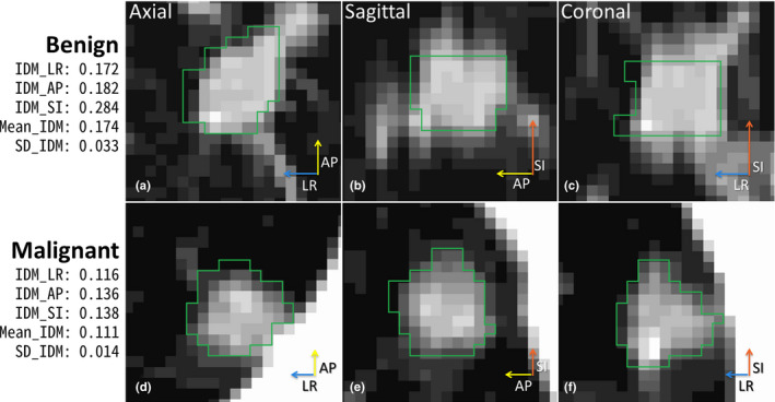
IDM and SD_IDM for small benign and malignant PNs (BB_AP = 10 mm for both). The length of each arrow indicates IDM value for left–right (LR), anterior–posterior (AP), and superior–inferior (SI) directions. [Color figure can be viewed at wileyonlinelibrary.com]

Figure 10.

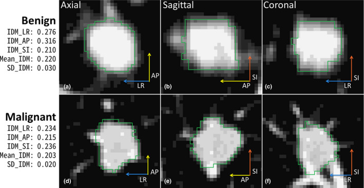
IDM and SD_IDM for large benign and malignant PNs (BB_AP = 17 mm for both). The length of each arrow indicates IDM value for the three directions. [Color figure can be viewed at wileyonlinelibrary.com]

4.B. Comparison with CADx systems

Table 4 shows the comparisons with CADx systems for lung cancer screening. The proposed method showed comparable or better accuracy than others. For both comparisons with CADx systems (Table 4) and with radiomics models (Table 5), when not specified ground‐truth was obtained by biopsy, resection, or 2‐year follow‐up. Also it should be noted that each method was evaluated on different datasets or with different validation methods. Most methods reported only AUC.

Table 4.

Comparison with CADx systems

	Dataset	Model description	Performance
Aoyama et al.14	76 primary lung cancer (73 patients) 413 benign (342 patients)	Automatic segmentation using dynamic programing LDA classification Leave‐one‐out CV	AUC 0.828 (single slice) AUC 0.846 (multiple slice)
Shah et al.16	35 solitary PNs 19 malignant and 16 benign PNs Pairs of CTs without contrast and with IV contrast	Attenuation, shape, and enhancement features (n = 31) LDA, quadratic discriminant analysis, logistic regession Leave‐one‐out CV	AUC 0.69–0.92
Suzuki et al.17	76 primary lung cancer (73 patients) 413 benign (342 patients)	Multiple massive training ANNs Integration ANN Leave‐one‐out CV	Sensitivity 100% Specificity 48% AUC 0.882
Way et al.19	256 PNs 124 malignant and 132 benign PNs (152 patients)	3D active contour segmentation Surface, demographic, and image features LDA and SVM two‐loop leave‐one‐out CV	AUC 0.857 (primary cancers) AUC 0.822 (metastatic cancers)
Han et al.21	LIDC 1356 PNs Ground‐truth by radiologist's assessment	Texture feature analysis SVM with radial basis function kernel 100 times hold‐out validation	AUC 0.839–0.927 Average AUC 0.894
LUNGx challenge10	LUNGx 10 patients calibration set and 60 patients testing set	SVM classification (n not reported) Trained by in‐house dataset; Independent cohort validation	CAD AUC 0.50–0.68 Observer AUC 0.70–0.85
Proposed SVM‐LASSO	LIDC 72 patients	2 important radiomic features LASSO features selection and SVM classification 10 × tenfold CV	Sensitivity 87.2% Specificity 81.2% Accuracy 84.6% AUC 0.89

Table 5.

Comparison with recently reported radiomics models

	Dataset	Model description	Sensitivity	Specificity	Accuracy	AUC
Hawkins et al.30	Baseline CT scans of 261 patients in NLST	23 RIDER stable radiomic features Random forest classifier 10 × 10‐fold CV	51.7%	92.9%	80.0%	0.83
Ma et al.31	LIDC 72 patients	583 radiomic features Random forest classifier 10‐fold CV	80.0%	85.5%	82.7%
Buty et al.32	LIDC 2054 PNs Ground‐truth by radiologist's assessment	Spherical Harmonics (100, 150, and 400 shape features) and AlexNet48 (4096 appearance features) Random forest classifier 10‐fold CV			82.4%
Kumar et al.33	LIDC 97 patients, including metastatic tumors	Deep convolutional neural network model (5000 features) 10‐fold CV	79.1%	76.1%	77.5%
Liu et al.36	172 patients (two independent cohorts 102 and 70 patients)	4 image traits selected from 24 image traits scored by radiologists Linear discriminant analysis Trained by 102 and tested by 70 pts	71.4%	83.7%	80.0%	0.81
Proposed SVM‐LASSO	LIDC 72 patients	2 important radiomic features LASSO features selection and SVM classification 10 × 10‐fold CV	87.2%	81.2%	84.6%	0.89

Aoyama et al.¹⁴ proposed segmentation‐based scheme which achieved 0.828 AUC (single slice) and 0.846 AUC (multiple slice). The performance (AUC 0.882) of Suzuki's scheme¹⁷ based on the multiple massive training ANNs was greater than that of Aoyama's scheme¹⁴ for the same database. Shah et al.¹⁶ applied contrast enhancement features extracted from pairs of CTs without contrast and with intravenous contrast injection. They achieved AUCs from 0.69 to 0.92 in a leave‐one‐out CV. Way et al.¹⁹ developed novel surface features, and the AUC was improved from 0.821 to 0.857 when the surface features were added to morphological and texture features. Han et al.²¹ achieved the highest AUC of 0.894, but it was the only study that ground‐truth was rated by radiologist's assessment. LUNGx Challenge reported the performance of 11 CAD systems (0.50–0.68 AUC) and six radiologists (0.70–0.85 AUC) for diagnosis of PNs on CT scans.¹⁰ Only three CAD methods performed statistically better than random guessing. Three radiologists performed statistically better than the best CAD system (0.68 AUC), which was based on SVM model.

4.C. Comparison with recently reported radiomics models

Table 5 shows the comparisons with recently reported radiomics models for lung cancer screening. The proposed method showed comparable or better accuracy than others. Some accuracy measurements were not reported in all studies.

Hawkins et al. proposed a random forest classifier using 23 stable (high reproducibility – concordance correlation coefficients ≥0.95 in test–retest) radiomic features.³⁰ Ma et al. proposed a random forest classifier using 583 radiomic features.³¹ Its performance on the same LIDC dataset as used in the present study was comparable to the proposed SVM‐LASSO model. However, the number of features used was more than eight times of the number of patients, which may cause a model overfitting problem.

Both Buty et al. and Kumar et al. applied deep learning techniques to predict malignancy of PNs.^{32, 33} Buty et al. extracted 4096 appearance features using the pretrained deep neural network (AlexNet⁴⁸) and 400 shape features from spherical harmonics. They fed these features into a random forest classifier, which achieved an accuracy of 82.4%.³² Since the neural network was pretrained using general color images, it is questionable that it can capture the salient features of a PN in the LDCT images. Kumar et al. used a deep neural network for both feature extraction and malignancy classification. They extracted a total of 5000 radiomic features and achieved an accuracy of 77.5%.³³ Deep learning is a rapidly emerging technology, but it needs large training dataset to avoid model overfitting because an intimidatingly large number of nodes and features are used. Liu et al. applied 24 image traits scored by radiologists to predict malignancy of PNs.³⁶ They achieved an accuracy of 80.0% and 0.81 AUC using four image traits that characterized PN size, contour/margin, concavity, and PNs in nontumor lobes. However, the image traits are semi‐quantitative with inter‐ and intra‐observer variation depending on radiologists' training and preferences.

Compared with the above methods, the main advantage of our method was that we used only two important features in the SVM‐LASSO model while achieving comparable or better accuracy.

4.D. Repeatability analysis

Using the group consensus contour from four manual segmentations is a good way to reduce inter‐observer variability; however, it is not representative of clinical practice where an automatic or semi‐automatic segmentation method with manual correction would be most likely used. In this study, we used the manual segmentations readily available and conducted a repeatability analysis across the four individual contours and the group consensus contours. First, we evaluated the inter‐observer agreement by comparing the individual contours and the consensus contour (Table S2). All the STAPLE‐estimated sensitivity, specificity, and Jaccard index were greater than 80% except the Jaccard index (77.7%) of R4. For feature agreement evaluation, we examined Bland–Altman plots⁴⁹ for BB_AP and SD IDM (Fig. S1) and calculated the intra‐class correlation coefficient (ICC)⁵⁰ between the consensus and individual contours. Figure S1 shows that the mean differences were close to zero, indicating that there was no systematic error, there was no trend in the plots, and the 95% limits of agreement were small. The ICCs were 0.95 for BB_AP and 0.78 for SD_IDM (Table S3), showing good agreement.⁵⁰ Lastly, Table S4 shows agreements in malignancy predictions between the consensus contours and individual contours. The predictions based on individual contours (80.6–83.6%) were slightly less accurate than the prediction based on the consensus contours (84.6%) but were not significantly different (all P > 0.05). Overall, the proposed method showed consistent results across different contours.

4.E. Limitations

Limitations of the present study include that the model was developed from a moderate‐size cohort of 72 patients, and there were no GGN cases in this cohort. Although ten‐, five‐, and twofold CV showed that the model was not notably affected by overfitting, the performance of the model should be validated in a larger, independent patient cohort. Also, there were no radiomic features that specifically characterized lobulated or spiculated margins.

4.F. Future work

In this study, we applied a feature discovery approach, which extracted a large number of image features (>100) first and then selected the most valuable ones that are independent, robust, and prominent in the data.²⁴ We plan to add a candidate feature approach, in which only a few important features are selected based on prior knowledge of their physiological, biochemical, or functional associations with the disease and therapy.²⁴ For example, quantification of lobulated or spiculated margins is a good candidate feature because it is known that a PN with smooth and well‐defined margins is more likely benign, while a PN with lobulated or spiculated margins is more likely malignant.⁵¹ A more accurate PN segmentation method is required to delineate lobulated or spiculated margins, and advanced feature extraction methods are needed to characterize such margins. Other potential candidate features include calcification, attachment, solidity, and cavitation of a PN.

It was difficult to diagnose small PNs (diameter = 6–15 mm and the probability of malignancy = 1–15%) based on radiomics features only. Our model achieved an accuracy of only 50% for PNs smaller than 15 mm. We showed that when combining plasma biomarkers with clinical variables and image features, the prediction was more accurate (AUC = 0.91 in Ref. [52] and 0.95 in Ref. [53]). These studies suggested that the biomarkers, clinical variables, and image features have complementary information. Therefore, we plan to integrate all these parameters in the SVM‐LASSO model and expect further improvement in the prediction accuracy, particularly for small PNs.

5. Conclusion

We developed an SVM‐LASSO model to predict malignancy of PNs with two CT radiomic features (the bounding box anterior–posterior dimension and the directional variation of local homogeneity). We demonstrated that the model achieved an accuracy of 84.6%, which was 12.4% higher than that for Lung‐RADS.

Conflict of Interest

The authors have no relevant conflicts of interest to disclose.

Supporting information

Table S1. The significant distinctive features by univariate analysis. The two features in bold were selected in the final model.

Table S2. Inter‐observer variation in contouring the PN volume. The STAPLE‐estimated sensitivity, specificity, and Jaccard index measured the agreement between the individual contours and the group consensus contours.

Table S3. The intra‐class correlation coefficient (ICC) among the individual contours and the group consensus contours.

Table S4. Comparison between the predictions by the SVM‐LASSO model using features from the group consensus contours and each radiologist's contours. P‐values were computed by McNamer's test between predictions based on the consensus and individual contours.

Figure S1. Bland–Altman plots for the two selected features between the group consensus contours and individual contours. Blue line is average difference and red dashed lines are 95% limits of agreement.

References

- 1. Aberle DR, DeMello S, Berg CD, et al. Results of the two incidence screenings in the National Lung Screening Trial. N Engl J Med. 2013;369:920–931. [DOI] [PMC free article] [PubMed] [Google Scholar]
- 2. McKee BJ, Regis SM, McKee AB, Flacke S, Wald C. Performance of ACR Lung‐RADS in a Clinical CT Lung Screening Program. J Am Coll Radiol. 2015;12:273–276. [DOI] [PubMed] [Google Scholar]
- 3. Pinsky PF, Gierada DS, Black W, et al. Performance of Lung‐RADS in the National Lung Screening Trial: a retrospective assessment. Ann Int Med. 2015;162:485–491. [DOI] [PMC free article] [PubMed] [Google Scholar]
- 4. Patz EF Jr., Pinsky P, Gatsonis C, et al. Overdiagnosis in low‐dose computed tomography screening for lung cancer. JAMA Int Med. 2014;174:269–274. [DOI] [PMC free article] [PubMed] [Google Scholar]
- 5. Armato SG, Giger ML, Moran CJ, Blackburn JT, Doi K, MacMahon H. Computerized detection of pulmonary nodules on CT scans. Radiographics. 1999;19:1303–1311. [DOI] [PubMed] [Google Scholar]
- 6. Doi K. Current status and future potential of computer‐aided diagnosis in medical imaging. Br J Radiol. 2005;78:s3–s19. [DOI] [PubMed] [Google Scholar]
- 7. Suzuki K. A review of computer‐aided diagnosis in thoracic and colonic imaging. Quant Imag Med Surg. 2012;2:163–176. [DOI] [PMC free article] [PubMed] [Google Scholar]
- 8. El‐Baz A, Beache GM, Gimel'farb G, et al. Computer‐aided diagnosis systems for lung cancer: challenges and methodologies. Int J Biomed Imaging. 2013;2013:46 [DOI] [PMC free article] [PubMed] [Google Scholar]
- 9. Choi W, Choi T‐S. Automated pulmonary nodule detection based on three‐dimensional shape‐based feature descriptor. Comput Methods Progr Biomed. 2014;113:37–54. [DOI] [PubMed] [Google Scholar]
- 10. Armato SG III, Drukker K, Li F, et al. LUNGx challenge for computerized lung nodule classification. J Med Imag. 2016;3:044506. [DOI] [PMC free article] [PubMed] [Google Scholar]
- 11. Gurney JW, Swensen SJ. Solitary pulmonary nodules: determining the likelihood of malignancy with neural network analysis. Radiology. 1995;196:823–829. [DOI] [PubMed] [Google Scholar]
- 12. Kawata Y, Niki N, Ohmatsu H, et al. Quantitative surface characterization of pulmonary nodules based on thin‐section CT images. IEEE Trans Nucl Sci. 1998;45:2132–2138. [Google Scholar]
- 13. McNitt‐Gray MF, Hart EM, Wyckoff N, Sayre JW, Goldin JG, Aberle DR. A pattern classification approach to characterizing solitary pulmonary nodules imaged on high resolution CT: preliminary results. Med Phys. 1999;26:880–888. [DOI] [PubMed] [Google Scholar]
- 14. Aoyama M, Li Q, Katsuragawa S, Li F, Sone S, Doi K. Computerized scheme for determination of the likelihood measure of malignancy for pulmonary nodules on low‐dose CT images. Med Phys. 2003;30:387–394. [DOI] [PubMed] [Google Scholar]
- 15. Armato SG, Altman MB, Wilkie J, et al. Automated lung nodule classification following automated nodule detection on CT: a serial approach. Med Phys. 2003;30:1188–1197. [DOI] [PubMed] [Google Scholar]
- 16. Shah SK, McNitt‐Gray MF, Rogers SR, et al. Computer aided characterization of the solitary pulmonary nodule using volumetric and contrast enhancement features. Acad Radiol. 2005;12:1310–1319. [DOI] [PubMed] [Google Scholar]
- 17. Suzuki K, Li F, Sone S, Doi K. Computer‐aided diagnostic scheme for distinction between benign and malignant nodules in thoracic low‐dose CT by use of massive training artificial neural network. IEEE Trans Med Imaging. 2005;24:1138–1150. [DOI] [PubMed] [Google Scholar]
- 18. Way TW, Hadjiiski LM, Sahiner B, et al. Computer‐aided diagnosis of pulmonary nodules on CT scans: segmentation and classification using 3D active contours. Med Phys. 2006;33:2323–2337. [DOI] [PMC free article] [PubMed] [Google Scholar]
- 19. Way TW, Sahiner B, Chan HP, et al. Computer‐aided diagnosis of pulmonary nodules on CT scans: improvement of classification performance with nodule surface features. Med Phys. 2009;36:3086–3098. [DOI] [PMC free article] [PubMed] [Google Scholar]
- 20. Lee MC, Boroczky L, Sungur‐Stasik K, et al. Computer‐aided diagnosis of pulmonary nodules using a two‐step approach for feature selection and classifier ensemble construction. Art Intell Med. 2010;50:43–53. [DOI] [PubMed] [Google Scholar]
- 21. Han F, Wang H, Zhang G, et al. Texture feature analysis for computer‐aided diagnosis on pulmonary nodules. J Digit Imaging. 2015;28:99–115. [DOI] [PMC free article] [PubMed] [Google Scholar]
- 22. Lambin P, Rios‐Velazquez E, Leijenaar R, et al. Radiomics: extracting more information from medical images using advanced feature analysis. Eur J Cancer. 2012;48:441–446. [DOI] [PMC free article] [PubMed] [Google Scholar]
- 23. Aerts HJWL, Velazquez ER, Leijenaar RTH, et al. Decoding tumour phenotype by noninvasive imaging using a quantitative radiomics approach. Nat Commun. 2014;5:4006. [DOI] [PMC free article] [PubMed] [Google Scholar]
- 24. Lu W, Chen W. Positron emission tomography/computerized tomography for tumor response assessment—a review of clinical practices and radiomics studies. Transl Cancer Res. 2016;5:364–370. [DOI] [PMC free article] [PubMed] [Google Scholar]
- 25. Gillies RJ, Kinahan PE, Hricak H. Radiomics: images are more than pictures, they are data. Radiology. 2016;278:563–577. [DOI] [PMC free article] [PubMed] [Google Scholar]
- 26. Scrivener M, de Jong EEC, van Timmeren JE, Pieters T, Ghaye B, Geets X. Radiomics applied to lung cancer: a review. Transl Cancer Res. 2016;5:398–409. [Google Scholar]
- 27. Tan S, Kligerman S, Chen W, et al. Spatial‐temporal [(18)F]FDG‐PET features for predicting pathologic response of esophageal cancer to neoadjuvant chemoradiation therapy. Int J Radiat Oncol Biol Phys. 2013;85:1375–1382. [DOI] [PMC free article] [PubMed] [Google Scholar]
- 28. Zhang H, Tan S, Chen W, et al. Modeling pathologic response of esophageal cancer to chemoradiation therapy using spatial‐temporal (18)F‐FDG PET features, clinical parameters, and demographics. Int J Radiat Oncol Biol Phys. 2014;88:195–203. [DOI] [PMC free article] [PubMed] [Google Scholar]
- 29. Lu W, Tan S, Chen W, et al. Pre‐chemoradiotherapy FDG PET/CT cannot identify residual metabolically‐active volumes within individual esophageal tumors. J Nucl Med Radiat Ther. 2015;6:226. [DOI] [PMC free article] [PubMed] [Google Scholar]
- 30. Hawkins S, Wang H, Liu Y, et al. Predicting malignant nodules from screening CTs. J Thorac Oncol. 2016;11:2120–2128. [DOI] [PMC free article] [PubMed] [Google Scholar]
- 31. Ma J, Wang Q, Ren Y, Hu H, Zhao J. Automatic lung nodule classification with radiomics approach. Paper presented at: SPIE Medical Imaging 2016: PACS and Imaging Informatics: Next Generation and Innovations2016; San Diego, California, United States.
- 32. Buty M, Xu Z, Gao M, Bagci U, Wu A, Mollura DJ. Characterization of lung nodule malignancy using hybrid shape and appearance features. In: Ourselin S, Joskowicz L, Sabuncu MR, Unal G, Wells W, eds. Medical Image Computing and Computer‐Assisted Intervention – MICCAI 2016: 19th International Conference, Athens, Greece, October 17–21, 2016, Proceedings, Part I, vol. 9900. Cham: Springer International Publishing; 2016:662–670. [Google Scholar]
- 33. Kumar D, Shafiee MJ, Chung AG, Khalvati F, Haider MA, Wong A. Discovery Radiomics for Computed Tomography Cancer Detection. arXive preprint. 2015:arXiv:1509.00117.
- 34. Balagurunathan Y, Kumar V, Gu Y, et al. Test‐retest reproducibility analysis of lung CT image features. J Dig Imaging. 2014;27:805–823. [DOI] [PMC free article] [PubMed] [Google Scholar]
- 35. Balagurunathan Y, Gu Y, Wang H, et al. Reproducibility and prognosis of quantitative features extracted from CT images. Transl Oncol. 2014;7:72–87. [DOI] [PMC free article] [PubMed] [Google Scholar]
- 36. Liu Y, Balagurunathan Y, Atwater T, et al. Radiological image traits predictive of cancer status in pulmonary nodules. Clin Cancer Res. 2016;23:1442–1449. [DOI] [PMC free article] [PubMed] [Google Scholar]
- 37. Armato SG III, McLennan G, Bidaut L, et al. The lung image database consortium (LIDC) and image database resource initiative (IDRI): a completed reference database of lung nodules on CT scans. Med Phys. 2011;38:915–931. [DOI] [PMC free article] [PubMed] [Google Scholar]
- 38. Ibanez L, Schroeder W, Ng L, Cates J. The ITK Software Guide. Clifton Park: Kitware; 2005. [Google Scholar]
- 39. Warfield SK, Zou KH, Wells WM. Simultaneous truth and performance level estimation (STAPLE): an algorithm for the validation of image segmentation. IEEE Trans Med Imaging. 2004;23:903–921. [DOI] [PMC free article] [PubMed] [Google Scholar]
- 40. Choi W, Xue M, Lane BF, et al. Individually optimized contrast‐enhanced 4D‐CT for radiotherapy simulation in pancreatic ductal adenocarcinoma. Med Phys. 2016;43:5659–5666. [DOI] [PMC free article] [PubMed] [Google Scholar]
- 41. Choi W, Choi T‐S. Genetic programming‐based feature transform and classification for the automatic detection of pulmonary nodules on computed tomography images. Inf Sci. 2012;212:57–78. [Google Scholar]
- 42. Pagano M, Gauvreau K. Principles of Biostatistics, 2nd edn. Pacific Grove, CA: Duxbury; 2000. [Google Scholar]
- 43. Haralick RM, Shanmugam K, Dinstein I. Textural features for image classification. IEEE Trans Syst Man Cybern. 1973;3:610–621. [Google Scholar]
- 44. Galloway MM. Texture analysis using gray level run lengths. Comput Graph Image Process. 1975;4:172–179. [Google Scholar]
- 45. Tang X. Texture information in run‐length matrices. IEEE Trans Image Process. 1998;7:1602–1609. [DOI] [PubMed] [Google Scholar]
- 46. Ward JH Jr.. Hierarchical Grouping to Optimize an Objective Function; 2012.
- 47. Lin H‐T, Lin C‐J, Weng RC. A note on Platt's probabilistic outputs for support vector machines. Mach Learn. 2007;68:267–276. [Google Scholar]
- 48. Krizhevsky A, Sutskever I, Hinton GE. ImageNet Classification with Deep Convolutional Neural Networks. Paper presented at: Advances in Neural Information Processing Systems; 2017.
- 49. Bland JM, Altman DG. Agreement between methods of measurement with multiple observations per individual. J Biopharm Stat. 2007;17:571–582. [DOI] [PubMed] [Google Scholar]
- 50. Parmar C, Rios Velazquez E, Leijenaar R, et al. Robust radiomics feature quantification using semiautomatic volumetric segmentation. PLoS One. 2014;9:e102107. [DOI] [PMC free article] [PubMed] [Google Scholar]
- 51. Erasmus JJ, Connolly JE, McAdams HP, Roggli VL. Solitary pulmonary nodules: part I. Morphologic evaluation for differentiation of benign and malignant lesions. Radiographics. 2000;20:43–58. [DOI] [PubMed] [Google Scholar]
- 52. Ma J, Guarnera MA, Zhou W, Fang H, Jiang F. A prediction model based on biomarkers and clinical characteristics for detection of lung cancer in pulmonary nodules. Transl Oncol. 2016;10:40–45. [DOI] [PMC free article] [PubMed] [Google Scholar]
- 53. Lin Y, Leng Q, Jiang Z, et al. A classifier integrating plasma biomarkers and radiological characteristics for distinguishing malignant from benign pulmonary nodules. Int J Cancer. 2017;141:1240–1248. [DOI] [PMC free article] [PubMed] [Google Scholar]
Associated Data
This section collects any data citations, data availability statements, or supplementary materials included in this article.
Supplementary Materials