Multimodal MR Synthesis via Modality-Invariant Latent Representation

Abstract

We propose a multi-input multi-output fully convolutional neural network model for MRI synthesis. The model is robust to missing data, as it benefits from, but does not require, additional input modalities. The model is trained end-to-end, and learns to embed all input modalities into a shared modality-invariant latent space. These latent representations are then combined into a single fused representation, which is transformed into the target output modality with a learnt decoder. We avoid the need for curriculum learning by exploiting the fact that the various input modalities are highly correlated. We also show that by incorporating information from segmentation masks the model can both decrease its error and generate data with synthetic lesions. We evaluate our model on the ISLES and BRATS datasets and demonstrate statistically significant improvements over state-of-the-art methods for single input tasks. This improvement increases further when multiple input modalities are used, demonstrating the benefits of learning a common latent space, again resulting in a statistically significant improvement over the current best method. Lastly, we demonstrate our approach on non skull-stripped brain images, producing a statistically significant improvement over the previous best method. Code is made publicly available at https://github.com/agis85/multimodal brain synthesis.

I. Introduction

Medical imaging technology is an important component of modern health care, and is widely used for diagnosis and treatment. There are a plethora of medical imaging techniques (e.g. X-ray, CT, MRI), and each has its own characteristics and nuances. Moreover, within Magnetic Resonance Imaging (MRI) technique, it is often possible to obtain images using different settings that essentially accentuate T1 and T2 content in the underlying tissue. In this work, we refer to these images of different contrast as modalities, and refer to our approach as multimodal (which in the context of MRI is seen as also multi-parametric). Image synthesis has attracted a lot of attention recently due to exciting potential applications in medical imaging: synthesised data for example may be used to impute missing images (e.g., as in [1]), to derive images lacking a particular pathology, which is not present in the input modality (for detection purposes, e.g., [2], [3]), to perform attenuation correction (e.g., [4], [5]), to improve algorithm performance on other medical imaging tasks, such as image segmentation and registration [1], [6], and others.

The current state of the art methods in image synthesis learn mappings between pairs of image modalities [7], [8], [9]. However, it is often the case that we have several modalities available (a typical clinical MR protocol collects a multitude of images), and taking advantage of their collective information could potentially improve synthetic results. In fact, different modalities highlight different anatomy (or pathology) in the body and, by using them together, it is possible to obtain better synthesis results through information sharing. For this reason, state-of-the-art methods use multi-input architectures [9] and obtain higher quality synthetic images. On the other hand, if a specific number of input modalities is mandatory for a model, then this reduces the number of applicable cases to the ones strictly containing this complete set of image modalities. To overcome this we propose a multi-input (and multi-output) deep neural network, which does not require all inputs in order to synthesise outputs, but can make use of additional inputs, when available, to achieve enhanced accuracy.

In this paper we propose a deep fully convolutional neural network model for MR synthesis. By synthesis here we mean a model that takes a number of images, showing the same organs in different modalities, as input, and outputs synthetic images of that same anatomy in one or more new modalities. We approach the task using deep neural networks as they have previously produced impressive results in a large range of image processing tasks [10], [11], including promising results for brain synthesis [7]. This is likely due to their ability to automatically learn richly structured hierarchical features [12].

Our model takes aligned images as input¹, making use of multiple modalities when available, allowing users to simply provide any of the available modalities at test time. We show that it outperforms state of the art neural network and random forest methods when trained on a single modality, with results improving further when additional modalities are given as input. Our end-to-end model, depicted in Figure 1, processes input images in three stages: encoding, representation fusion, and decoding. As each of these stages is independent, our model is modular, i.e. encoders and/or decoders can be added to accommodate additional modalities. Our contributions are:

1. We present a novel modular convolutional deep network for MR image synthesis that improves the quality of images synthesised from a single input modality compared to current leading methods.

2. We show that our model can combine information from multiple inputs to further improve synthesis quality.

3. By using a single shared decoder for each output modality and a custom loss function, we are able to learn a modality-invariant latent representation to which all input modalities are mapped. This renders the model robust to missing inputs, and avoids the need for curriculum learning [14] during training.

4. We encourage the latent representation to capture the useful information in a simple way by restricting the size of the decoders.

5. We demonstrate that the model can be easily extended to new output modalities through the addition of decoders which can be trained in isolation.

6. We improve synthesis errors of pathological images by including information from lesion segmentation masks. In this setting, our model can also generate on request images with synthetic lesions by adding the affected region as defined by a segmentation mask.

7. We show that the model works for both skull-stripped and non skull-stripped brain data, with no change required, demonstrating that the latent representation is flexible, and not overly tailored to a specific task.

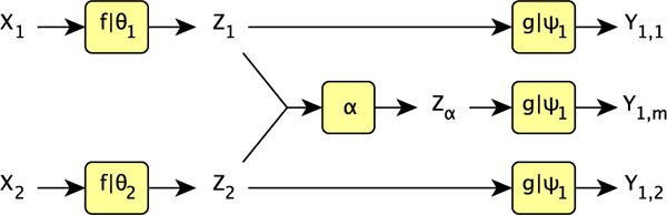
Fig. 1.

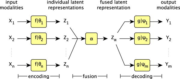
Schematic for our model. X₁, …, X_n represent the n input modalities and Y₁, …, Y_m represent the m output modalities. The f represent encoders, parametrised by their respective θ_i, which map inputs into latent representations, α fuses those latent representations, and the decoders g, each parametrised by their own ψ_j, decode the representation into outputs. Full details of each component is given in the main text.

The paper is organised as follows. Section II reviews relevant prior work. Section III discusses the requirements of a multi-input fusion method. Section IV details our model. Section V describes experimental setup and datasets used. We present results in Section VI, and conclude in Section VII.

II. Previous Work

Machine vision techniques have been extensively used in MR image processing for image synthesis. They can be broadly divided into those that use only one input modality (unimodal) and those that use more (multimodal). We discuss these below and mention some limitations. Since in the multimodal case latent representation learning becomes important, we also review key machine learning literature on this topic.

Unimodal

MR synthesis has often been treated as a patch-based regression task [15], [16], [3], [17]. In this setting mappings are learnt, using various techniques, which take a patch of an image or volume in one modality, and predict the intensity of the central pixel of the corresponding patch in a target modality. The performance of these approaches has been shown to be aided by the addition of hand-crafted features that capture elements of the global structure of the image [9].

Another common approach to synthesis is the use of an atlas, such as in [16], [2], [18]. Here, rather than learning a mapping, an atlas of image pairs is leveraged, and reconstructing a new volume from a source modality is achieved by matching the volume with the entries in the atlas of the same modality, and constructing the synthetic images from the corresponding atlas images in the target modality.

A sparse dictionary representation of the source and target modality has been proposed in [19], which synthesises new images with patch matching. In [20], joint dictionary learning is used to learn a cross-modality dictionary of the pair of source and target modalities that minimises the statistical distribution between them via optimisation. Image synthesis has also been treated directly as an optimisation problem in an unsupervised setting [8]. The target modality candidates are generated by a search method and then combined to obtain a synthetic image.

More recently, neural networks have been applied to MR synthesis and segmentation, and like many of the sparse coding based methods, often they approach the problem as a patch based regression [21]. The Location Sensitive Deep Network (LSDN) [7] is a patch-based neural network that, given as input a patch and its spatial position within the volume, can learn a position-dependent intensity map between two modalities. Motivated by the observation that conditioning on the location in the volume greatly reduces the complexity of the intensity transforms needing to be learnt, LSDN has been shown to produce state of the art MR synthesis results. Another neural network approach is [22], in which a deep encoder-decoder network synthesises images of a target modality.

Neural networks have also been employed to synthesise pseudo-healthy images. In [23], a denoising variational autoencoder was used to synthesise pseudo-healthy images for the purpose of image registration. Using the denoising mechanism of [24], the variational autoencoder of [23] models lesions as noise, learning to synthesise images without damaged tissues.

One main drawback of these approaches is their inability to robustly exploit multiple input modalities. In addition, patch- and atlas-based methods can be prohibitively slow at test time. Further, the overhead of having many unimodal models from an application standpoint is significant since all these different models have to be trained and maintained. Certainly, there could be a benefit to learning a single multi-purpose model.

Multimodal synthesis

Multimodal image analysis is on the rise, as evidenced by recent multimodal analysis methods for example to solve segmentation (e.g. [25], [26]) or classification (e.g. [27]) tasks. This is natural as the inputs image the same subject, but provide different information to be exploited.

The single input, multi-output method, Extended Modality Propagation [28], warrants mention. Unlike related methods, where the input is expected to be an image in some source modality, in [28] the input is a label map, which delineates the areas of interest (e.g., white and grey matter), and the algorithm synthesises multimodal images accordingly. However, it uses a single input and solves a somewhat different problem.

Although for segmentation rather than synthesis, Hetero-Modal Image Segmentation (HeMIS), a convolutional neural network model, uses a robust fusion method to address the challenge of missing input data [26]. We discuss this approach in more detail in Section IV-E, and use their proposed multi-input fusion method as a benchmark in our experiments.

The model we propose here addresses the challenge of multi-input, multi-output synthesis, and does so in a robust way: outperforming existing approaches, and, when inputs are missing, performing as well as a model trained specifically for that fewer input case. Central to our approach to multimodal data is the embedding of inputs into a latent space, and we now review key relevant literature on this task.

Shared representation learning

Perhaps one of the reasons that multimodal synthesis has been difficult to accomplish is the need to map data into a common shared representation. Previous work on multimodal data fusion and shared representation in neural networks [29] has shown the plausibility of shared latent representations for generative tasks. There has also been relevant work on common representation learning, in which different data types are embedded into a common representation space. Key early work on multimodal learning that was robust to missing data is the multimodal autoencoder [30], in which a bimodal deep autoencoder was learnt for audio and video data of speech. This model could reconstruct both modalities from either the audio or the video, and was trained by minimising this reconstruction error. However, as noted in [31], there is no direct learning signal encouraging a shared common representation. In an attempt to address these shortcomings Correlational Neural Networks [31] both directly encourage correlation in the common representation space, and minimise the cross reconstruction error. However, their current formulation restricts them to the bi-modal setting, due to the use of explicit correlation calculations.

Here we are interested in fusing any number of modalities, and we do not use the formulation of Correlational Neural Network directly. Instead, as our inputs are already similar, in that they are all images of the same organ, are aligned and differ only in intensity patterns, we propose a simple method of training that enforces the same constraints: minimising reconstruction error and the distance between the embeddings in the common space, which indirectly maximises the correlation. Thus, our approach is broadly similar to the statistical regularisation approach in [32], in which cross-modal scene representations are learnt. However, in [32], the regularisation is done by encouraging the latent representation activations for all modalities to follow the same distribution. Whereas here, as the various inputs are sufficiently similar, we directly encourage the activations to be equal. Our approach to latent representation learning is detailed in Section IV-D.

III. Fusion Requirements

Many synthesis approaches learn to synthesise one modality from another. Thus, when n modalities are being considered, there exist n(n − 1) possible one input one output synthesis tasks, and a separate model would be required for each one. This approach not only becomes infeasible as n grows, it also does not benefit from other input sources despite the fact they may be available. On the other hand, if the accuracy of a model is improved by leveraging multiple input modalities, but all inputs are required, the applicability is reduced to only those situations in which all required modalities are available.

The challenge is to build a model which can take as input any subset of the n image modalities to produce its output. The model we introduce here achieves this goal by approaching the task in three stages. Firstly, all inputs are projected into a shared latent representation space, then these latent representations are fused into a single representation and, finally, mapped to the required output modality. The fusion step, (detailed in Sections IV-B and IV-E), can be performed on any number of latent representations and having all of the input modalities improves results.

IV. Proposed Approach

Our proposed model is a fully convolutional deep neural network, that can map multiple input modalities to multiple output modalities. It takes as input full 2D volume slices of any subset of its inputs, and synthesises the corresponding 2D slices in all output modalities. The model is trained end-to-end with gradient descent, and simultaneously learns both encoders and decoders. Through the use of a multi-component cost function the model is encouraged to learn latent representations that balance modality-invariance with the retention of modality specific information. During the fusion step, the latent representations produced by each of the encoders are combined to form a single latent representation, which is then decoded to produce the final output. Below, we will first describe the three sections of our model in order: encoders, fusion method, and decoders. We then discuss in depth the importance of learning good latent representations, and detail our multi-component cost function, providing the motivations for each component.

A. Encoding

We learn one independent encoder for each input modality of our model, with an architecture as shown in Figure 2. The encoders embed single-channel input images into a multichannel latent space. Specifically, if our input images are slices of size W × H then out latent representation is an L channel image of that same size. We took inspiration from U-Net [33] to make our encoder modules. The idea behind the U-Net’s down-sampling followed by up-sampling and skip connection architecture is to allow the network to exploit information at larger spatial scales than those of the filters, whilst also not losing useful local information. In addition, skip connections facilitate gradient flow during training, as discussed in [34]. Our encoders are shallower than the original U-Net having only two downsample (and upsample) steps compared to U-Net’s four downsample (and upsample) steps. This reduces the training and run times for the model. Although the final quality of synthesis shown herein already outperforms the compared approaches, it may be possible to decrease the error further through the use of deeper encoders. We also replaced the ReLU [35] in the standard U-Net with Leaky ReLU [36], as we found that the network is easier to train and it improves the quality of the latent representations.² Throughout the network, we use a stride of 1, and pad the images by repeating the border pixels so that the final output has the same width and height as the original input. An encoder f is trained for each input modality X_i to learn the set of parameters θ_i (the network’s weights) that fully describes the map from the i-th input modality to the latent space Z_i. In our model we use a 16-channel latent representation. Experiments with different latent representation sizes showed that this produced good results, whilst keeping the model small enough to easily train (see Section VI-A).

Fig. 2.

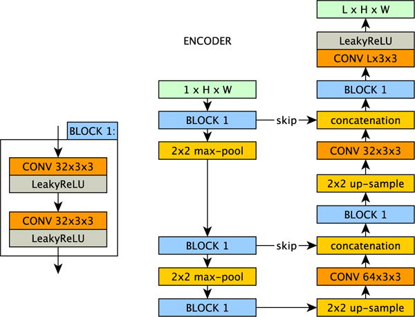
Our U-Net [33] like encoder(s) f(·|θ). Each input modality i has its own encoder, parametrised by θ_i, that maps the input image in modality i to the latent space Z_i. We use L = 16 channels in the latent space.

B. Fusion

During the fusion step, our model uses a fusion operation, α, to combine each of the individual representations produced by the encoders into a single fused representation, which we call Z_α. It is this fusion step that gives the model its robustness to missing input data. In theory, α could be chosen to be any function that takes as input any number of latent representations, and returns a single fused latent representation. We want this fused representation to integrate information present in the various inputs, in a way that we not only preserve commonly represented features, but also retain unique features expressed in one modality but not the others. Additionally, the fused representation should be robust to varying numbers of inputs and if some input modalities are missing, it should accommodate such missing inputs. Specifically, the aim is that, given any subset of latent representations, we produce a fused latent representation that is at least as good as each of the constituent latent representations, in terms of synthesis quality.

To this end, we use the pixel-wise max function (1) to combine our latent representations into a fused latent representation. The use of the max means that, in each channel, each pixel of the latent representation has exactly the value of the corresponding pixel in one of the original latent representations. In particular, if the signal is large and positive in one constituent latent representation, then it will be chosen for the fused representations. Our fusion operator α is defined as:

$$Z_{\alpha }=\alpha (Z_1,\dots Z_n)=\mathit{\text{max}}(Z_1,\dots Z_n),$$ (1)

for n input modalities and corresponding individual latent representations. The fused representation is exactly the same size and shape as the individual latent representations Z_i. The performance of this fusion method is intimately linked with the nature of the latent representations learnt, which is detailed in Section IV-D. Note that the use of max does not bias the method towards bright final outputs, as the intensities of the synthesised image depend on the decoding step.

Although we use max fusion in our model, there is potential to learn the fusion operation itself, for example by learning an additional hyper-parameter that interpolates between mean and max fusion. This may further regularise the model as non-max fusion allows gradient from the fused output to flow to all inputs, rather than just the max.

C. Decoding

The decoding stage of the model uses a fully-convolutional network to map the latent representation to a target output modality. Here the input is a multi-channel image-sized latent representation, and the output is a single channel image of the required modality. The exact architecture of our decoder g is shown in Figure 3. We train one decoder for each output modality m, learning the parameters ψ_j, i.e. the network’s weights, to map the latent space Z_α to the j-th output modality. We kept the decoder shallower than the encoder to encourage the latent representation to contain the useful information in a simple way. Deeper decoders showed no considerable improvement, whilst increasing the computational overhead.

Fig. 3.

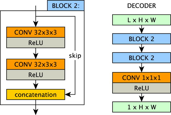
The decoder module g(·|ψ), which is built from two residual blocks. Each output modality j has its own decoder, parametrised by ψ_j, that maps latent representations to the outputs of that modality. In our experiments we set the channels in the latent space L to be 16.

D. Learning Modality-Invariant Latent Representations

The nature of the latent representation learnt by our model depends critically on the cost function used to train it. We train our network to minimise a cost function constituted from three cost components which we will introduce below. The final cost drives the network to achieve three goals:

1. Each modality’s individual latent representation should produce all outputs as accurately as possible.

2. The latent representations from all input modalities should be close in the Euclidean sense.

3. The fused latent representation resulting from α should produce all outputs as accurately as possible.

Together these constraints are sufficient to ensure that our architecture works well with a variety of fusion operations, as well as our pixel-wise max approach discussed in IV-B.

It is the fusion step that gives the model its robustness to missing input data as the fusion operation α, can be applied to any number of latent representations, and always yields a single fused latent representation. However, the quality of this fused representation depends critically on both the latent representations produced by the encoders, and the nature of this fusion operation. As noted in [31], simply embedding inputs into the same representation space does not ensure that they share a meaningful latent representation. The embeddings, if not encouraged to do so, have no reason to use the latent space in a comparable way. If this is the case, then decoding one latent representation is distinct from decoding the other, and moreover, fusion becomes difficult, as operations such as taking the mean are no longer meaningful. Another way to state this same problem is that, if the different embeddings use the latent space in different ways, then in order to know how to decode a latent representation, you need to know from which modality it originally came, i.e. the meaning of the latent representation is dependent on its initial modality. Thus, in order to overcome this issue we need to produce a latent representation that is independent of the originating modality.

Let $Z_i^k$ be the latent representation of image k in modality i, i.e. $Z_i^k=f(X_i^k|{\theta }_i)$. One requirement of our model is that any input alone should produce good synthesis results, since the model should work well with any subset of inputs, including a single input. Thus, if $Y_j^k$ is the k-th image in our target output modality j, then we want $g(Z_i^k|{\psi }_j)$ to equal $Y_j^k$ for every input modality i. Essentially, each modality’s individual latent representation should produce all outputs as accurately as possible, when decoded.

Cost component c₁

This desire gives rise to the first component of our cost function. Given n input and m output modalities then our model is fully described by the parameters for the n encoders θ = θ₁, …, θ_n, and the parameters for the m decoders, ψ = ψ₁, …, ψ_m. We define c₁ as:

$$c_1(k|\mathit{\theta },\psi )=\frac{1}{m}{\displaystyle \sum _{i=1}^n{\displaystyle \sum _{j=1}^m\mathit{\text{MAE}}(g(f(X_i^k|{\theta }_i)|{\psi }_j),Y_j^k)}}$$ (2)

where $X_i^k$ is the k-th slice of input in modality i, $Y_j^k$ is the corresponding slice in output modality j, and MAE is the mean absolute error, where here the mean is taken over all pixels in the image. Note that we divide by m to average over all outputs. Thus, this cost can be seen as the sum of each input modality’s average reconstruction error across all outputs.

Note that decoders, g, are shared, i.e. for each output modality there is exactly one decoder, which is used to decode the latent representations from each of the input modalities. This provides some encouragement for the encoders to come to a shared, modality-invariant representation during training. However, due to the highly non-linear, non-injective nature of the decoder, it is possible for very different latent representations (i.e. ones with a large Euclidean distance between them) to be decoded into very similar output images. Thus, although (2) encourages the latent representations to be mutually compatible with a shared decoder, it does not necessarily result in embeddings that share the same semantics. In order to ensure that we can meaningfully fuse latent representations, we exploit the fact that the input images are already highly correlated, since they are images of the same subject, and we directly encourage the encoders for the different modalities to produce similar embeddings for a given image.

Cost component c₂

To this end, we introduce a second cost that captures the desire that representations from all input modalities should be similar. Although what we really mean by similar here is related to both the details of the fusion operation α and the decoder, we encourage the representations to be close under the Euclidian norm, as if they are sufficiently similar under this metric they will also be sufficiently similar in the required way. In order to bring all of the latent representations together, we minimise their mean pixel-wise variance (c and p index the channels and pixels respectively):

$$c_2(k|\mathit{\theta })=\frac{1}{|C||P|}{\displaystyle \sum _{c\in C}{\displaystyle \sum _{p\in P}\mathit{\text{var}}(f{(X_1^k|{\theta }_1)}_{p,c},\dots ,}f{(X_n^k|{\theta }_n)}_{p,c})}$$ (3)

Cost component c₃

Although c₁, c₂ encourage the encoders to learn a shared, modality-independent latent representation, so far there is nothing to encourage this representation to be especially suitable for the fusion operation α used in the model. In fact, so far the particular fusion method chosen has no bearing on the training of the network. The shared representation learnt should be admissible for a wide range of fusion options, but if we decide on a fusion operation in advance, then there is potential to learn a shared representation that works particularly well with that fusion method. As well as meeting the two constraints from above, there may also be sufficient flexibility in the final representation for it to specialise towards the fusion operation in use. To this end, we include a final component in our cost function:

$$c_3(k|\mathit{\theta },\psi )=\frac{1}{m}{\displaystyle \sum _{j=1}^m\mathit{\text{MAE}}}(g(\alpha (f(X_1^k|{\theta }_1),\dots ,(f(X_n^k|{\theta }_n))|{\psi }_j),Y_j^k)$$ (4)

to directly encourage the minimisation of the reconstruction error from the fused representation. This is the only one of the three costs that involves the fusion operation α.

E. Other Approaches to Fusion

Our multi-component cost function encourages modality-invariant, yet informative, latent representation that can be used with a variety of fusion techniques. Here we discuss alternatives to our pixel-wise max approach (which we also compare with in our experiments).

Latent mean fusion

One simple way to fuse a number of latent representations is to average over them. With this approach to fusion, the final fused latent representation is simply the pixel-wise mean of the individual latent representations.

$$Z_{\alpha }=\mathit{\text{mean}}(Z_1,\dots Z_n)$$ (5)

This approach should work well if the individual latent representations are approximately noisy versions of a common latent representation. On the other hand, in situations where in one of the input modalities it is possible to detect details that cannot be seen in the others, this averaging would smooth out these details. Also, it is unable to preferentially select specific input modalities. Therefore, the information in the latent representation from a highly informative input could be partially lost through averaging with the latent representations from several other less informative inputs.

HeMIS-like fusion

One approach to the creation of a fused latent representation, introduced in [26], is to define the latent representation as the concatenation of the mean and variance of the individual latent representations Z_i.

$$Z_{\alpha }=\mathit{\text{concat}}(\mathit{\text{mean}}(Z_1,\dots Z_n),\mathit{\text{var}}(Z_1,\dots Z_n))$$ (6)

This method was shown in [26] to work very well for image segmentation, producing state of the art results. Our experiments using this fusion showed competitive results also for modality synthesis. HeMIS uses both the mean and the variance over the individual representations as its fused latent representation, and thus the decoder has information about where the latent representations most disagree, as well as their average value. However, it is still the case that all input representations contribute equally to the final latent representation. Unlike max fusion, HeMIS-like fusion can’t explicitly rely on more informative inputs. To achieve a 16-channel latent representation with this method we generate eight channels with the encoder, so that the concatenation of the mean and variance is sixteen channels.

Output mean

As a final baseline, we also compare with the results produced by taking the average of the synthesised images decoded from each individual latent representation Z₁, …, Z_n independently. Thus, instead of decoding a fused representation to get a single synthesised output, we decode each individual representation into a synthetic image and take the average of those individual images.

V. Experimental Setup

Datasets

We use three datasets to test our model. Firstly we used 28 pre-processed volumes from the Ischemic Stroke Lesion Segmentation (ISLES) 2015 challenge.³ The volumes have been skull-stripped and re-sampled to an isotropic spacing of 1mm³ (SISS) resp. and co-registered to the FLAIR sequences. The provided volumes were imaged in T1w, T2w, FLAIR and DWI. We also used data from the multimodal Brain Tumour Segmentation (BRATS) 2015⁴ challenge. Data are skull-striped, co-aligned, and interpolated to 1mm³ resolution. The dataset consists of high and low grade glioma cases, from which we used the latter containing 54 volumes, imaged in T1w, T1c, T2w, and FLAIR. Both datasets are released with segmentation masks of lesions. Finally, we used 28 volumes from the Information eXtraction from Images (IXI) dataset⁵, which contains co-registered T1, T2 and PD-weighted images from healthy subjects, in order to evaluate our method in non skull-stripped images. Our architecture uses 2D slice of the volumes. If not otherwise stated, we use axial-plane slices for our experiments (examples of which are in Figure 5).

Fig. 5.

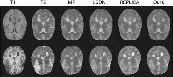
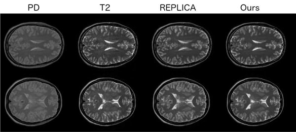
Comparison of the unimodal models for T 1 → T 2 on a healthy and unhealthy test case. The columns show the input image, the target output image and then the synthesis results of MP, LSDN, REPLICA, and our model respectively. The first row is for a healthy brain, and the second row shows the results on a brain with a large lesion.

Pre-Processing

We perform all experiments on the data at its full resolution, trimming excess border pixels resulting in volumes of 224 × 160 pixel images for the ISLES dataset, 240 × 240 for the BRATS dataset and 256 × 256 for the IXI dataset. Trimming is done to remove uninformative background areas, and is done in such a way that the resulting image size is divisible by 4, so that the two 2 × 2 max-pooling, followed by the two 2 × 2 upsampling operations of the encoder do not change the image size. We keep all slices, which is ≈ 150, although the number of slices differs slightly between volumes. As a final pre-processing step we normalise each volume by dividing by the volume’s average intensity. As well as centralising all the volumes across all modalities to a mean of 1, this also keeps all values positive, all background values as 0, and maintains the slight differences in volume variance seen between healthy and unhealthy volumes. For our DeepMedic [25] test, we instead normalised the data by subtracting the mean and dividing by the standard deviation, as this is a requirement for the model.

Training and Implementation Details

We train our model w.r.t. a cost function given by the three constituent parts described in Section IV-D. Our final cost function is:

$${\displaystyle \sum _{t=1}^3{\displaystyle \sum _{k\in K}{c}_t}}(k|\mathit{\theta },\psi ).$$ (7)

where K is the set of images in the current minibatch.

The model is trained using Adam [37] with default parameters, to minimise the cost w.r.t the parameters θ and ψ. We use a batch size of 16 images. All our code is written in Python with Keras⁶, and we run it using the Theano backend [38] on a single NVidia Titan X GPU. We train all models using 5-fold cross-validation. For each cross-validation split, we divide the datasets into training, validation (used to determine when to stop training to avoid overfitting), and test examples. In each fold different test and validation volumes are used, and the remaining volumes are used for training. In the case of ISLES the training, validation and test sets consist of 22, 3 and 3 volumes respectively, with one unhealthy volume in each of the validation and test sets, and the remaining 7 in the training set. For BRATS, the training, validation and test sets consist of 42, 6 and 6 volumes respectively, except when using FLAIR images, when we excluded three volumes from the training set as large portions of those volumes were missing in the FLAIR data. For IXI, we use 22 volumes for training, 3 for validation and 3 for testing. Training takes around one hour for each ISLES and IXI split and two hours for each BRATS split. When trained, synthesising a volume with our model takes approximately one second.

Once the model has been trained its test-time structure is that shown in Figure 1. However, during training additional outputs are required for calculation of the cost in eq. 7, and thus the network has the layout shown in Figure 4.

Fig. 4.

The setup of the model during training for a two input one output case. As we are dealing with a single output there is only one decoder, g|ψ₁, used three times: once to decode each of the two individual latent representations Z₁, Z₂, and once to decode the fused representation Z_α. At test time we use the synthesis result from the fused representation as our output. Here we write Y_1,i to mean output modality Y₁ synthesised from latent representation Z_i.

Benchmark Methods Details

As well as comparing the results of our model with those produced by the various fusion approaches discussed in section IV-E we also compare with three synthesis methods detailed below:

Modality Propagation (MP)

This is a standard benchmark for synthesis methods [2], which we implemented in Python to include as a baseline. All parameters are taken from the original paper. As it is prohibitively slow to synthesise a volume, and it has been shown that the method is outperformed by LSDN [7], we run MP on the ISLES dataset to show that it performs as expected, that is, with a slightly higher mean squared error that LSDN. See Table II for details.

TABLE II.

T1 → T2 and T1 → FLAIR Synthesis From Unimodal Models On Isles Dataset

T2	MP [2]	LSDN [7]	REPLICA [9]	Proposed
MSE	0.397 (0.15)	0.345 (0.12)	0.325 (0.12)	0.299 (0.11)
SSIM	0.798 (0.02)	0.811 (0.03)	0.823 (0.24)	0.831 (0.03)
PSNR	25.22 (0.96)	25.22 (1.36)	25.51 (1.20)	25.78 (1.39)

FLAIR	MP [2]	LSDN [7]	REPLICA [9]	Proposed
MSE	0.343 (0.12)	0.286 (0.10)	0.301 (0.11)	0.268 (0.10)
SSIM	0.802 (0.03)	0.820 (0.03)	0.814 (0.03)	0.831 (0.04)
PSNR	28.81 (2.13)	29.61 (2.17)	29.43 (2.25)	29.99 (2.24)

Location Sensitive Deep Network (LDSN)

We implemented the LSDN as described in [7]. Specifically, we implemented the larger 400,40 neuron version (referred to as LSDN-2 in the paper) without the shrink-connect optimisation, as this is the variant shown to produce the best results in the paper. We train the model to minimise the mean squared error using stochastic gradient descent with a batch size of 128. This approach is slightly outperformed by [8] from the same authors. Here we compare with LSDN, as both LSDN and our approach are neural network based.

Regression Ensembles with Patch Learning for Image Contrast Agreement (REPLICA)

Our final baseline method is REPLICA [9], a supervised random forest image synthesis approach which uses multi-scale features to achieve accurate synthesis results. As this method is able to handle multi-input situations, we compare it to our model in unimodal and multimodal settings. We implemented REPLICA in Python.

Evaluation metrics

To evaluate the performance of the methods, we use mean squared error (MSE), structural similarity index (SSIM) and peak signal-to-noise ratio (PSNR). Given two volumes $y,\widehat{y}\in Y$, where y is the ground-truth image in the output modality, and $\widehat{y}$ is the prediction, the MSE is computed as: $\mathit{\text{MSE}}(\widehat{y},y)=|{\mathrm{\Omega }}_Y{|}^{-1}{\displaystyle {\sum }_{x\in {\mathrm{\Omega }}_Y}{(\widehat{y}(x)-y(x))}^2}$ where Ω_Y is the set of 3D coordinates of pixels for modality Y, and |Ω_Y| is the number of voxels in Ω_Y. SSIM is computed as: $\mathit{\text{SSIM}}(\widehat{y},y)=\frac{(2{\mu }_{\widehat{y}}{\mu }_y+c_1)(2{\sigma }_{\widehat{y}y}+c_2)}{({\mu }_{\widehat{y}}^2+{\mu }_y^2+c_1)({\sigma }_{\widehat{y}}^2+{\sigma }_y^2+c_2)}$ where μ_y and ${\sigma }_y^2$ are the mean and variance of volume y and ${\sigma }_{\widehat{y}y}$ the covariance between the volume y and the prediction. Finally, PSNR is computed as: $10{\log }_{10}(\frac{MA{X}_I^2}{\mathit{\text{MSE}}})$, where MAX_I is the maximum pixel value of the image.

Significance tests

In order to assess our results we compare our method to the best baseline method in each experiment using a paired t-test and testing for significance at the 5% level. Significant results are shown in bold in the tables.

VI. Results and Discussion

Here we present the results of a series of experiments examining our proposed model and comparing it to other approaches. In VI-A we first perform experiments to determine the number of channels to use in our latent representation. In VI-B we show the performance of our model on unimodal synthesis. Subsequently, in VI-C we demonstrate that adding inputs increases performance. We also demonstrate robustness to missing inputs comparing against individual models trained specifically for the inputs present. In VI-D we show the importance of each of the three components of our cost function. Next, in VI-E, we proceed to demonstrate that we can train a new decoder for an unseen output without learning a new latent representation. In VI-F we show that our model can be used with other fusion methods. In VI-G we demonstrate that our model also works for non skull-stripped data. In VI-H we show that segmentation masks can be used to further improve our model’s results, and that they permit the generation of synthetic lesions. In VI-I we show that our model can synthesise images from views not seen during training, and also demonstrate that our synthetic volumes have off-plane consistency.

A. Latent representation size

We first ran experiments to determine the best latent representation size. Table I results show that the 16 channel latent representation outperforms both the 4 and 8 channel versions statistically significantly in both MSE and PSNR, and also by a small margin in SSIM. Thus, as the 16 channel representation achieves the best results, while keeping the network’s size manageable, we use it for our model in all experiments. Although we could optimally tune the latent representation size for each experimental setup, here we are interested in demonstrating that a single model can perform well in a range of tasks, and thus fix the latent representation size throughout.

TABLE I.

Comparison of different sized latent Representations For T1, T2, DWI → FLAIR

	4 channels	8 channels	16 channels
MSE	0.184 (0.07)	0.191 (0.08)	0.171 (0.06)
SSIM	0.866 (0.02)	0.865 (0.02)	0.869 (0.02)
PSNR	31.61 (1.69)	31.50 (1.72)	31.10 (1.59)

B. Unimodal synthesis

In our first experiment we train two unimodal models to generate T2 and FLAIR images respectively from T1 inputs. We repeat the experiment for the ISLES and BRATS dataset and compare our models with the benchmark methods described in Section V. The results are presented in Tables II and III and show that our model outperforms the other methods. In addition, statistically significant differences are produced on the ISLES dataset for SSIM, and on the BRATS dataset for all metrics. Examples images are shown in Figure 5.

TABLE III.

T1 → T2 AND T1 → FLAIR SYNTHESIS FROM UNIMODAL MODELS ON BRATS DATASET

T2	LSDN [7]	REPLICA [9]	Proposed
MSE	0.449 (0.12)	0.573 (0.17)	0.333 (0.13)
SSIM	0.909 (0.02)	0.901 (0.01)	0.929 (0.17)
PSNR	30.12 (1.62)	28.62 (1.69)	30.96 (1.85)

FLAIR	LSDN [7]	REPLICA [9]	Proposed
MSE	0.332 (0.16)	0.432 (0.17)	0.283 (0.14)
SSIM	0.887 (0.01)	0.870 (0.01)	0.897 (0.01)
PSNR	29.68 (1.56)	28.32 (1.38)	30.32 (1.61)

C. Multimodal synthesis

To assess the performance of our method on multiple inputs we compare two experimental setups using the ISLES dataset, with T1, T2, DWI as inputs, and FLAIR as output. In Experiment A we train distinct instances of our model for each possible combination of T1, T2, and DWI inputs, synthesising FLAIR in all the cases. Thus, in total we train 7 different models: 3 unimodal, 3 bi-modal, and 1 tri-modal. As a baseline comparison we also train 7 REPLICA models for the same tasks. In Experiment B we take our trained tri-modal model from Experiment A, and at test time, provide different subsets of the inputs (e.g. only T1 images, only T2 and DWI images, etc), to evaluate robustness to missing inputs.

The results of both setups are reported in Table IV, and a test example is shown in Figure 6. In the table we show in bold results where REPLICA is outperformed with statistical significance. Overall, in all three experiments, we observe the positive effect of multimodal inputs. With our model, this gain does not penalise flexibility as its performance when data is missing (Experiment B) is never worse than the performance of a model trained specifically for the fewer input case (Experiment A). This demonstrates that our model, due to the effectiveness of the latent representation, is able to exploit the input modalities when available, without becoming reliant on them. Our model outperforms REPLICA in 6 of the 7 experimental setups, with statistically significant improvements in 5 cases, when using one model with missing inputs (Table IV).

TABLE IV.

Synthesis of FLAIR images when training in the experiment A and experiment B Setups.

Combinations of Input			MSE (FLAIR modality)
T1	T2	DWI	REPLICA	Proposed: Exp. A	Proposed: Exp. B
✓	—	—	0.301 (0.11)	0.268 (0.10)	0.249 (0.09)
—	✓	—	0.374 (0.16)	0.328 (0.14)	0.321 (0.12)
—	—	✓	0.278 (0.09)	0.303 (0.13)	0.285 (0.13)
—	✓	✓	0.235 (0.08)	0.215 (0.09)	0.214 (0.09)
✓	—	✓	0.225 (0.08)	0.208 (0.09)	0.198 (0.02)
✓	✓	—	0.271 (0.12)	0.218 (0.08)	0.214 (0.08)
✓	✓	✓	0.210 (0.08)	0.171 (0.06)	0.171 (0.06)
Average:			0.271	0.244	0.236

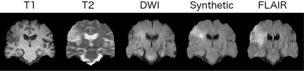
Fig. 6.

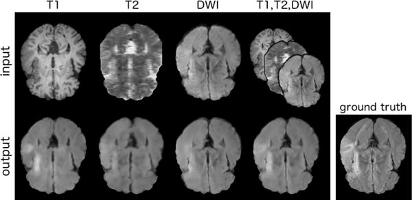
Example multimodal synthesis from our model, using all three inputs to synthesise FLAIR. The first row shows the T1, T2 and DWI inputs respectively. In the second row, the images below each input show the synthesis result from that input’s latent representation alone (i.e. single input results), the fourth image shows the synthesis result from the fused latent representation, and the final image is the FLAIR ground-truth.

This experiment’s setup also allows us to compare our model for different input combinations. Three observations can be made: Firstly, T2 alone gives the highest error, and all other input combinations, (including T1 alone and DWI alone) result in statistically significant improvements over just T2. Secondly, in all two-input cases, the results are better than the results for the constituent modalities individually, and this improvement is also statistically significant in each case (e.g. when T1 and DWI are given as input the results outperform those for either T1 or DWI alone). Lastly, when T1, T2 and DWI are all provided as input the results are significantly better than in all other cases. To summarise: in all cases adding an additional input modality resulted in a statistically significant improvement, when compared to the results without that additional input. It is worth noting that, as all outputs are coming from the same fixed FLAIR decoder, these significant differences can be understood both as significant differences in the final outputs, and/or as significant differences in the fused latent representations. We also visualise the behaviour of our max-fusion operator α in the three input case, (Figure 7). As can be seen, all inputs contribute to the final fused latent representation, and the contributions of the different modalities are not related to tissue classes in a simple way.

Fig. 7.

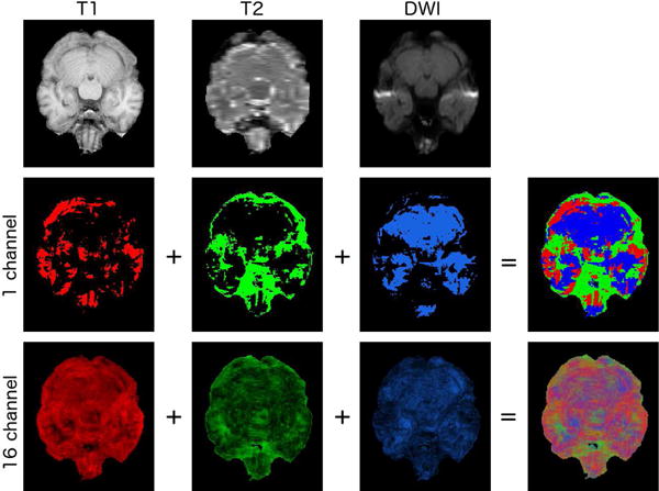
Visualisation of the max-fusion behaviour, showing from which inputs the values in the latent representation originate. As can be seen, there is no simple relationship between the input selected and the underlying anatomy. The first row shows T1, T2 and DWI inputs. The first three images in the second row show, for a single channel, the pixels of the individual latent representations that are selected from the max-fusion operator. The fourth image shows the three results simultaneously, with pixels coming from T1, T2 and DWI shown in red, green and blue respectively. The final row is the same as the second row, but rather than showing the results for a single channel, it shows the result averaged over all 16. Note that this figure shows only which inputs are chosen, not the values of the latent representations themselves.

D. Influence of each cost component

Here we demonstrate that the robustness seen previously stems from the composition of our cost function. To show this, we evaluate the effect of each of the three components described in Section IV-D by assessing model performance when each component is individually removed. We train three models for synthesising FLAIR from T1, T2, DWI using the ISLES dataset, each with one of the cost components removed. These results, along with the results for training with the full cost function are shown in Table V. The best result is achieved when all cost components are employed. Specifically, without c₁ the synthesis result is very good when the model has all inputs, but considerably worse when inputs are missing. Without c₂, the results for single inputs are good, but results with multiple inputs are worse. Finally, when component c₃ is excluded from the cost, there is a slight degradation in the results with a single missing input, and when all three inputs are given the model is significantly worse. Thus, it can be seen that our multi-component cost enables the model to achieve high accuracy whilst retaining robustness to missing data.

TABLE V.

Synthesis of FLAIR images when training with different cost functions

Inputs			MSE (FLAIR)
T1	T2	DWI	all costs	no c1	no c2	no c3
✓	—	—	0.249 (0.09)	0.546 (0.19)	0.261 (0.10)	0.250 (0.10)
—	✓	—	0.321 (0.12)	0.903 (0.47)	0.331 (0.14)	0.316 (0.13)
—	—	✓	0.285 (0.13)	0.497 (0.19)	0.293 (0.14)	0.286 (0.13)
—	✓	✓	0.214 (0.09)	0.324 (0.16)	0.262 (0.12)	0.276 (0.11)
✓	—	✓	0.198 (0.02)	0.252 (0.10)	0.240 (0.09)	0.228 (0.09)
✓	✓	—	0.214 (0.08)	0.329 (0.12)	0.345 (0.17)	0.277 (0.10)
✓	✓	✓	0.171 (0.06)	0.185 (0.08)	0.176 (0.07)	0.278 (0.11)
Average:			0.236	0.434	0.273	0.273

The influence of the cost components can also be seen visually in the latent representations learnt by our model, see Figure 8. Observe the similarity of all latent representations achieved by minimising their variance through cost function component eq. (3). At the same time the fusion operation α, preserves unique information across the latent components corresponding to bright pixels of the individual latent representations. Note that these bright pixels represent strong features, and do not necessarily correspond to bright pixels in the output.

Fig. 8.

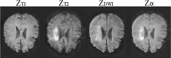
A channel from the 16-channel latent representation of our model with T1, T2, DWI inputs. The first three images show the latent representations learnt by the three inputs, T1, T2, DWI respectively. The fourth column shows the fused representation. The high-intensity regions in Z_T2, which correspond to lesions, are preserved in the fused representation Z_α despite the latent representations Z_T1 and Z_DWI showing minimal or no lesion information.

E. Adding new decoders

One aim of our latent representations is to introduce modality invariance. This should allow adding inputs and outputs to an already trained network, with minimal performance change. Here we demonstrate that an additional output can be appended to an already trained network. We train a model with inputs T1 and T2, and outputs DWI and Flair. At test time, the mean squared error of DWI images is 0.218. Next, we train another model with the same inputs, but only Flair as output; to this already trained model, we add just a DWI decoder that we then train in isolation. The test error for DWI was 0.263, which is ∼ 17% higher, and not a statistically significant difference, compared with the previous case.

F. Alternative fusion operations

In this experiment we demonstrate that our model is still effective with other fusion methods, such as those described in Section IV-E. To this end, we train one model for each of these fusion methods with T1, T2, and DWI as inputs, and FLAIR as output on the ISLES dataset. We get the best MSE with our max fusion method, which is equal to 0.171. HeMIS MSE is 0.178, while latent and output mean follow with 0.187 and 0.193 respectively. We also experiment with missing inputs with the HeMIS and latent mean fusion methods. On average, across all seven input combinations, our model achieved an MSE of 0.236 as shown in Table V, whereas HeMIS and latent mean achieved 0.239 and 0.246 respectively, demonstrating that the model still works well with missing inputs in these cases, but performs best with our suggested fusion approach.

G. Non skull-stripped data

In these experiments we explore the model in situations where the brain data has not been skull-stripped. As also discussed in [9], synthesising non skull-stripped volumes is difficult because of the intensity inhomogeneity in MR images caused by the dark skull regions surrounded by bright skin and fat regions. REPLICA [9], which is being used as a baseline has been demonstrated to be effective on non skull-stripped data, producing state of the art results, and we compare our method with this approach for evaluation. For this experiment we use 28 volume pairs of PD-weighted and T2 modalities of the IXI dataset. The results are given in Table VI. As can be seen, our method outperforms REPLICA, with statistical significance, in all three error metrics. Non skull-stripped example results are shown in Figure 9. Although we initially used 28 subjects to be comparable to the ISLES dataset size, to demonstrate that our model scales well and benefits from more training data we trained our model on the full IXI dataset, which consists of 577 volumes (347 training, 115 validation and 115 testing). This significantly improved the performance (compare with Table VI), with MSE dropping to 0.067, and SSIM and PSNR rising to 0.872 and 35.20 respectively.

TABLE VI.

Results from PD to T2 synthesis on the non skull-stripped IXI dataset.

	REPLICA [9]	Proposed
MSE	0.293 (0.05)	0.129 (0.04)
SSIM	0.854 (0.03)	0.865 (0.03)
PSNR	28.93 (1.20)	32.92 (1.06)

Fig. 9.

Non skull-stripped synthesis examples. The two rows show slices from different test volumes. The columns show the input PD image, the ground truth T2 image, the REPLICA synthetic T2 and our model’s synthetic T2 respectively. Our method can be seen to produce more accurate outputs.

H. Augmenting inputs with segmentation masks

The ISLES dataset includes segmentation masks that delineate unhealthy regions. We provide the segmentation mask as an additional input channel. With this augmented input, the model can directly modulate its behaviour on affected regions. Specifically, when we train a network with DWI input and FLAIR output, we obtain a MSE of 0.303. When we train a similar network where the mask is provided as an extra channel in the input, the MSE reduces to 0.290. Even though the improvement is in the range of ≈ 3%, we observed that affected regions in the synthesised images are sharper (also note unhealthy regions are only a small part of a few volumes).

With the same augmented inputs, we can also generate synthetic lesions. To achieve this at test time, we use the lesion mask from an unhealthy brain on a healthy brain, and then run the synthesis as normal. A visual example is shown in Figure 10. We then train DeepMedic [25] to segment lesions using the FLAIR modality of the ISLES dataset as input. In order to test the quality of our synthetic images, we use DeepMedic to segment the synthetic lesion and get ≈ 84% accuracy (Dice coefficient) on a single test-case.

Fig. 10.

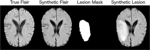
Synthesis of a lesion by including a segmentation mask when synthesising an otherwise healthy image. This subject is taken from ISLES dataset in the FLAIR modality.

I. View-transfer synthesis

We demonstrate that our architecture can synthesise images (at test time) taken from a different perspective of the 3D volume. Here, we train a model with T1, T2 and DWI inputs and FLAIR output on axial-plane slices as normal, but we test on coronal view slices. An example result is shown in Figure 11. Observe that the synthetic image contains all the details including the ischemic lesion, seen in the other modalities and in the ground-truth FLAIR image, visually demonstrating transfer learning capabilities w.r.t. the point of views (axial-coronal planes in this example). Finally, as our method synthesises volumes slice by slice, we evaluate intensity consistency between slices in off-plane reconstructions. As the examples in Figure 12 show, consistency is good.

Fig. 11.

A visual demonstration of robustness of our model to view transfer. We take the model trained on axial-plane slices and test using coronal-plane slices (shown). The image show the T1, T2 and DWI input slices, the synthesised FLAIR slice, and the ground-truth FLAIR image respectively.

Fig. 12.

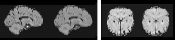
Off-plane reconstruction examples. The volume was constructed by synthesising axial slices. Sagittal and coronal slices are taken from this reconstructed volume and compared them to ground truth images. From left to right, the images show a target T1 image, and the off-plane reconstruction, a target FLAIR image, and the corresponding off-plane reconstruction.

VII. Conclusion

We proposed a multi-input, multi-output end-to-end deep convolutional network for synthesis of MR images, capable of fusing information contained in different modalities. Most current synthesis approaches are single-input single-output and thus do not take advantage of the correlated information available within clinical exams. We designed a modular architecture composed of three parts: encoder, latent representation fusion, and decoder. These modules are learnt end-to-end, using a cost function that encourages representations to be modality-invariant, whilst the individual reconstruction error is kept low.

When trained with a single input, our method outperforms the current best methods in all three metrics in each experiment. In particular, significantly outperforming in SSIM in all experiments, and in all metrics on the BRATS dataset. We also demonstrate improved performance on non skull-stripped brain images compared to previous methods. When more inputs are added, the error is further reduced, and our approach is shown to outperform REPLICA statistically significantly in all multi-input experiments. We also show in our experiments that our architecture and cost function can be used in conjunction with various fusion methods, including the one proposed in HeMIS [26], and the model can be trained end-to-end without the need for the added complexity of curriculum learning [14]. We also demonstrate that the model is robust to missing inputs: for any subset of inputs it performs as well as a model trained specifically for the subset. Central to our design is the quest towards modality-invariant latent representations. This is achieved by via a cost function that aims to unearth shared information whilst still preserving unique (to a specific input) semantics. Such modality invariance has many benefits such as the ability to train new decoders (as demonstrated in VI-E).

We used MSE, SSIM, and PSNR as evaluation criteria, but these may not directly reflect diagnostic quality. Investigations of new, useful for synthesis, metrics, is an ongoing process in the community. Application-specific metrics are also sought-after and our application driven DeepMedic-based evaluation of pseudo-lesion synthesis points to that direction. This work used three datasets independently, but there is potential for combining information across many sources. This has benefited deep learning in many domains: its application in our context requires that we find suitable pre-processing schemes to alleviate intensity distribution differences between the different sources. Finally, we opted for encoders/decoders that were “small” and fast but still performed exceptionally well. Fine-tuning their design could improve performance further.

Although our approach outperforms the baseline methods in all three metrics, the images produced by LSDN appear sharper than those produced by our method. We believe this is a result of LSDN independently processing small 3 × 3 × 3 voxel cubes to predict a single output voxel. However, although the LSDN approach promotes sharpness, the numerical results show sharpness does not necessarily translate to accuracy: it is certainly possible to have a very sharp, but inaccurate synthetic output. This said, we believe that in future work steps could be taken to improve sharpness of our model, for example through the use of perceptual similarity metrics [39].

Finally, our work here considers co-registered data and does not explore the effect of mis-registration between inputs. Recent preliminary findings on low resolution data, using a model similar to the one presented herein but with an additional registration layer [13], show that it is possible to add robustness to input misalignment.

In summary, we presented a multi-input, multi-output end-to-end deep convolutional network for synthesis of MR images, which we tested on three different brain datasets. We showed that the model is robust, performs well and can handle a variety of different challenges such as robustness to missing input, learning just a new decoder for an unseen modality and even synthesising new (unseen) views of the data. We see that such multimodal models could be well placed to impute data on large databases (e.g. biobanks) w.r.t unimodal approaches. From a deployment perspective they are less complex (one vs many different models to deploy/maintain), more flexible (new outputs can be added with minimal training) and more importantly are robust by taking advantage of information across input modalities, without being reliant on any of them.

References

- 1.van Tulder G, de Bruijne M. MICCAI. Springer; 2015. Why does synthesized data improve multi-sequence classification? pp. 531–538. [Google Scholar]
- 2.Ye DH, Zikic D, Glocker B, Criminisi A, Konukoglu E. MICCAI. Springer; 2013. Modality propagation: coherent synthesis of subject-specific scans with data-driven regularization; pp. 606–613. [DOI] [PubMed] [Google Scholar]
- 3.Bowles C, Qin C, Ledig C, Guerrero R, Gunn R, Hammers A, Sakka E, Dickie DA, Hernández MV, Royle N, et al. SASHIMI. Springer; 2016. Pseudo-healthy image synthesis for white matter lesion segmentation; pp. 87–96. [Google Scholar]
- 4.Burgos N, Cardoso MJ, Thielemans K, Modat M, Pedemonte S, Dickson J, Barnes A, Ahmed R, Mahoney CJ, Schott JM, et al. Attenuation correction synthesis for hybrid PET-MR scanners: application to brain studies. IEEE transactions on medical imaging. 2014;33(12):2332–2341. doi: 10.1109/TMI.2014.2340135. [DOI] [PubMed] [Google Scholar]
- 5.Roy S, Wang WT, Carass A, Prince JL, Butman JA, Pham DL. PET attenuation correction using synthetic CT from ultrashort echo-time MR imaging. Journal of Nuclear Medicine. 2014;55(12):2071–2077. doi: 10.2967/jnumed.114.143958. [DOI] [PMC free article] [PubMed] [Google Scholar]
- 6.Iglesias JE, Konukoglu E, Zikic D, Glocker B, Van Leemput K, Fischl B. MICCAI. Springer; 2013. Is synthesizing MRI contrast useful for inter-modality analysis? pp. 631–638. [DOI] [PMC free article] [PubMed] [Google Scholar]
- 7.Van Nguyen H, Zhou K, Vemulapalli R. MICCAI. Springer; 2015. Cross-domain synthesis of medical images using efficient location-sensitive deep network; pp. 677–684. [Google Scholar]
- 8.Vemulapalli R, Van Nguyen H, Kevin Zhou S. Unsupervised cross-modal synthesis of subject-specific scans. ICCV. 2015:630–638. [Google Scholar]
- 9.Jog A, Carass A, Roy S, Pham DL, Prince JL. Random forest regression for magnetic resonance image synthesis. Medical Image Analysis. 2017;35:475–488. doi: 10.1016/j.media.2016.08.009. [DOI] [PMC free article] [PubMed] [Google Scholar]
- 10.Long J, Shelhamer E, Darrell T. Fully convolutional networks for semantic segmentation. CVPR. 2015:3431–3440. doi: 10.1109/TPAMI.2016.2572683. [DOI] [PubMed] [Google Scholar]
- 11.Wang J, Yang Y, Mao J, Huang Z, Huang C, Xu W. CNN-RNN: A unified framework for multi-label image classification. CVPR. 2016:2285–2294. [Google Scholar]
- 12.LeCun Y, Bengio Y, Hinton G. Deep learning. Nature. 2015;521(7553):436–444. doi: 10.1038/nature14539. [DOI] [PubMed] [Google Scholar]
- 13.Joyce T, Chartsias A, Tsaftaris SA. MICCAI. Springer; 2017. Robust multi-modal MR image synthesis; pp. 347–355. [Google Scholar]
- 14.Bengio Y, Louradour J, Collobert R, Weston J. ICML. ACM; 2009. Curriculum learning; pp. 41–48. [Google Scholar]
- 15.Roy S, Chou YY, Jog A, Butman JA, Pham DL. SASHIMI. Springer; 2016. Patch based synthesis of whole head MR images: Application to EPI distortion correction; pp. 146–156. [DOI] [PMC free article] [PubMed] [Google Scholar]
- 16.Jog A, Roy S, Carass A, Prince JL. 2013 IEEE 10th International Symposium on Biomedical Imaging. IEEE; 2013. Magnetic resonance image synthesis through patch regression; pp. 350–353. [DOI] [PMC free article] [PubMed] [Google Scholar]
- 17.Huynh T, Gao Y, Kang J, Wang L, Zhang P, Lian J, Shen D. Estimating CT image from MRI data using structured random forest and auto-context model. IEEE transactions on medical imaging. 2016;35(1):174–183. doi: 10.1109/TMI.2015.2461533. [DOI] [PMC free article] [PubMed] [Google Scholar]
- 18.Jog A, Carass A, Roy S, Pham DL, Prince JL. MR image synthesis by contrast learning on neighborhood ensembles. Medical image analysis. 2015;24(1):63–76. doi: 10.1016/j.media.2015.05.002. [DOI] [PMC free article] [PubMed] [Google Scholar]
- 19.Roy S, Carass A, Prince JL. Magnetic resonance image example-based contrast synthesis. IEEE transactions on medical imaging. 2013;32(12):2348–2363. doi: 10.1109/TMI.2013.2282126. [DOI] [PMC free article] [PubMed] [Google Scholar]
- 20.Huang Y, Beltrachini L, Shao L, Frangi AF. SASHIMI. Springer; 2016. Geometry regularized joint dictionary learning for cross-modality image synthesis in magnetic resonance imaging; pp. 118–126. [Google Scholar]
- 21.Li R, Zhang W, Suk HI, Wang L, Li J, Shen D, Ji S. MICCAI. Springer; 2014. Deep learning based imaging data completion for improved brain disease diagnosis; pp. 305–312. [DOI] [PMC free article] [PubMed] [Google Scholar]
- 22.Sevetlidis V, Giuffrida MV, Tsaftaris SA. SASHIMI. Springer International Publishing; 2016. Whole image synthesis using a deep encoder-decoder network; pp. 97–107. [Google Scholar]
- 23.Yang X, Han X, Park E, Aylward S, Kwitt R, Niethammer M. SASHIMI. Springer International Publishing; 2016. Registration of pathological images; pp. 97–107. [DOI] [PMC free article] [PubMed] [Google Scholar]
- 24.Vincent P, Larochelle H, Bengio Y, Manzagol PA. Extracting and composing robust features with denoising autoencoders. ICML. 2008:1096–1103. [Google Scholar]
- 25.Kamnitsas K, Ledig C, Newcombe VF, Simpson JP, Kane AD, Menon DK, Rueckert D, Glocker B. Efficient multi-scale 3D CNN with fully connected CRF for accurate brain lesion segmentation. Medical Image Analysis. 2017;36:61–78. doi: 10.1016/j.media.2016.10.004. [DOI] [PubMed] [Google Scholar]
- 26.Havaei M, Guizard N, Chapados N, Bengio Y. MICCAI. Springer; 2016. HeMIS: Hetero-modal image segmentation; pp. 469–477. [Google Scholar]
- 27.Suk HI, Lee SW, Shen D, Initiative ADN, et al. Hierarchical feature representation and multimodal fusion with deep learning for AD/MCI diagnosis. NeuroImage. 2014;101:569–582. doi: 10.1016/j.neuroimage.2014.06.077. [DOI] [PMC free article] [PubMed] [Google Scholar]
- 28.Cordier N, Delingette H, Lê M, Ayache N. Extended modality propagation: Image synthesis of pathological cases. IEEE Transactions on Medical Imaging. 2016;35(12):2598–2608. doi: 10.1109/TMI.2016.2589760. [DOI] [PubMed] [Google Scholar]
- 29.Chen G, Srihari SN. Generalized K-fan multimodal deep model with shared representations. arXiv preprint arXiv:1503.07906. 2015 [Google Scholar]
- 30.Ngiam J, Khosla A, Kim M, Nam J, Lee H, Ng AY. Multimodal deep learning. ICML. 2011:689–696. [Google Scholar]
- 31.Chandar S, Khapra MM, Larochelle H, Ravindran B. Correlational neural networks. Neural computation. 2016 doi: 10.1162/NECO_a_00801. [DOI] [PubMed] [Google Scholar]
- 32.Castrejon L, Aytar Y, Vondrick C, Pirsiavash H, Torralba A. Learning aligned cross-modal representations from weakly aligned data. CVPR. 2016:2940–2949. [Google Scholar]
- 33.Ronneberger O, Fischer P, Brox T. U-Net: Convolutional Networks for Biomedical Image Segmentation. MICCAI. 2015:234–241. [Google Scholar]
- 34.Drozdzal M, Vorontsov E, Chartrand G, Kadoury S, Pal C. International Workshop on Large-Scale Annotation of Biomedical Data and Expert Label Synthesis. Springer; 2016. The importance of skip connections in biomedical image segmentation; pp. 179–187. [Google Scholar]
- 35.Nair V, Hinton GE. Rectified linear units improve restricted boltzmann machines. ICML. 2010:807–814. [Google Scholar]
- 36.Maas AL, Hannun AY, Ng AY. Rectifier Nonlinearities Improve Neural Network Acoustic Models. ICML. 2013:6. [Google Scholar]
- 37.Kingma D, Ba J. Adam: A method for stochastic optimization. arXiv preprint arXiv:1412.6980. 2014 [Google Scholar]
- 38.Theano Development Team. Theano: A Python framework for fast computation of mathematical expressions. arXiv e-prints. 2016 May;abs/1605.02688 [Google Scholar]
- 39.Dosovitskiy A, Brox T. Generating images with perceptual similarity metrics based on deep networks. arXiv preprint arXiv:1602.02644. 2016 [Google Scholar]