Theta band oscillations reflect more than entrainment: behavioral and neural evidence demonstrate an active chunking process

Abstract

Parsing continuous acoustic streams into perceptual units is fundamental to auditory perception. Previous studies have uncovered a cortical entrainment mechanism in the delta and theta bands (~1–8 Hz) that correlates with formation of perceptual units in speech, music, and other quasi-rhythmic stimuli. Whether cortical oscillations in the delta-theta bands are passively entrained by regular acoustic patterns or play an active role in parsing the acoustic stream is debated. Here we investigate cortical oscillations using novel stimuli with 1/f modulation spectra. These 1/f signals have no rhythmic structure but contain information over many timescales because of their broadband modulation characteristics. We chose 1/f modulation spectra with varying exponents of f, which simulate the dynamics of environmental noise, speech, vocalizations, and music. While undergoing magnetoencephalography (MEG) recording, participants listened to 1/f stimuli and detected embedded target tones. Tone detection performance varied across stimuli of different exponents and can be explained by local signal to noise ratio computed using a temporal window around 200 ms. Furthermore, theta band oscillations, surprisingly, were observed for all stimuli, but robust phase coherence was preferentially displayed by stimuli with exponents 1 and 1.5. We constructed an auditory processing model to quantify acoustic information on various timescales and correlated the model outputs with the neural results. We show that cortical oscillations reflect a chunking of segments, >200 ms. These results suggest an active auditory segmentation mechanism, complementary to entrainment, operating on a timescale of ~200 ms to organize acoustic information.

Graphical Abstract

Parsing continuous natural sounds into perceptual units is fundamental to auditory perception. We used magnetoencephalography to investigate how the human auditory system groups sounds with 1/f modulation spectra, which mimic modulation profiles of natural sounds and indicate irregular temporal structure. The results revealed an active chunking mechanism reflected by theta band oscillations.

Introduction

Cortical oscillations are entrained not only by strictly periodic stimuli but also by quasi-rhythmic structures in sounds, such as the amplitude envelope of speech (Luo & Poeppel, 2007; Kerlin et al., 2010; Cogan & Poeppel, 2011; Peelle et al., 2013; Zion Golumbic et al., 2013; Doelling et al., 2014; Kayser et al., 2015) and music (Doelling & Poeppel, 2015), the frequency modulation envelope (Henry & Obleser, 2012; Herrmann et al., 2013; Henry et al., 2014), and even abstract linguistic structure (Ding et al., 2015). These studies have advanced our understanding of how the auditory system exploits regular temporal structure to organize acoustic information. It is not clearly understood, though, whether cortical oscillations tracking sounds are a result of neural responses passively driven by rhythmic structures or reflect a built-in constructive processing scheme, namely that the auditory system employs a windowing process to actively group acoustic information (Ghitza & Greenberg, 2009; Ding & Simon, 2014).

It has been proposed that cortical oscillations in the auditory system reflect an active parsing mechanism - the auditory system chunks sounds into segments of around 150 – 300 ms, roughly a cycle of the theta band, for grouping acoustic information (Ghitza & Greenberg, 2009; Schroeder et al., 2010; Ghitza, 2012). A slightly different (but related) view hypothesizes that the auditory system processes sounds using temporal integration windows of multiple sizes concurrently: within a short temporal window (~ 30 ms), temporally fine-grained information is processed; a more ‘global’ acoustic structure is extracted within a larger temporal window (~ 200 ms) (Poeppel, 2003; Giraud & Poeppel, 2012). These frameworks are largely based on studying speech signals that contain these timescales as relatively obvious components: the temporal modulations of speech peak around 4–5 Hz (Ding et al., 2017). However, if such a segmentation scale or integration window exists at the timescale of ~ 200 ms in the auditory system intrinsically, then we should find evidence of its deployment even when the sounds have broadband spectra and are irregularly modulated over a wide range of timescales. In contrast, if cortical oscillations are solely or primarily stimulus-driven, one ought not to find robust oscillatory activity using such irregular sounds.

Natural sounds, such as environmental noise, speech, and some vocalizations, often have broadband modulation spectra that show a 1/f pattern: the modulation spectrum has larger power in the low frequency range and the modulation strength decreases as frequency increases (Voss & Clarke, 1978; Singh & Theunissen, 2003; Theunissen & Elie, 2014). This characteristic of modulation spectra can be delineated using a straight line at a logarithmic scale, with its exponent indicating how sounds are modulated across various timescales. For example, environmental noise has a relatively shallow 1/f modulation spectrum with an exponent of 0.5, while speech has a steeper spectrum with an exponent of f between 1 and 1.5 (Singh & Theunissen, 2003). As 1/f spectra reflect acoustic dynamics across many timescales, and not rhythmic structure centered at a narrow frequency range, 1/f stimuli are well suited to test how the auditory system spontaneously organizes acoustic information across various timescales.

We generated frequency modulated sounds having 1/f modulation spectra with different exponents, to imitate irregular dynamics in natural sounds (Garcia-Lazaro et al., 2006) and inserted a tone of short duration (50 ms) as a detection target. We recorded participants’ neurophysiological responses while they listened to the 1/f stimuli and detected the embedded tones. We were interested to see what timescale of acoustic information is used to detect salient changes (i.e. embedded tones) and at what frequencies robust oscillatory activity is evoked by irregular 1/f stimuli. We then used an auditory processing model to quantify acoustic information over different timescales. By employing mutual information analysis, we determine the timescale over which acoustic information is grouped. By designing our experiment in this manner, we are able to investigate the temporal structure imposed by the neural architecture of the auditory system to sample information from the environment.

Materials and Methods

Participants

Fifteen participants (age 23 – 49, one left-handed, eight females) took part in the experiment. Handedness was determined using the Edinburgh Handedness Inventory (Oldfield, 1971). All participants had normal hearing and no neurological deficits. Written informed consent was obtained from every participant before the experiment. The experimental protocol was approved by the New York University Institutional Review Board.

Stimuli and Design

We followed the methods used in Garcia-Lazaro et al. (2006) to generate similar (but modified) stimuli with modulation spectra of 1/f. A schematic plot of the stimulus generation process is shown in Fig. 1A.

Figure 1. Stimulus generation and modulation power spectrum.

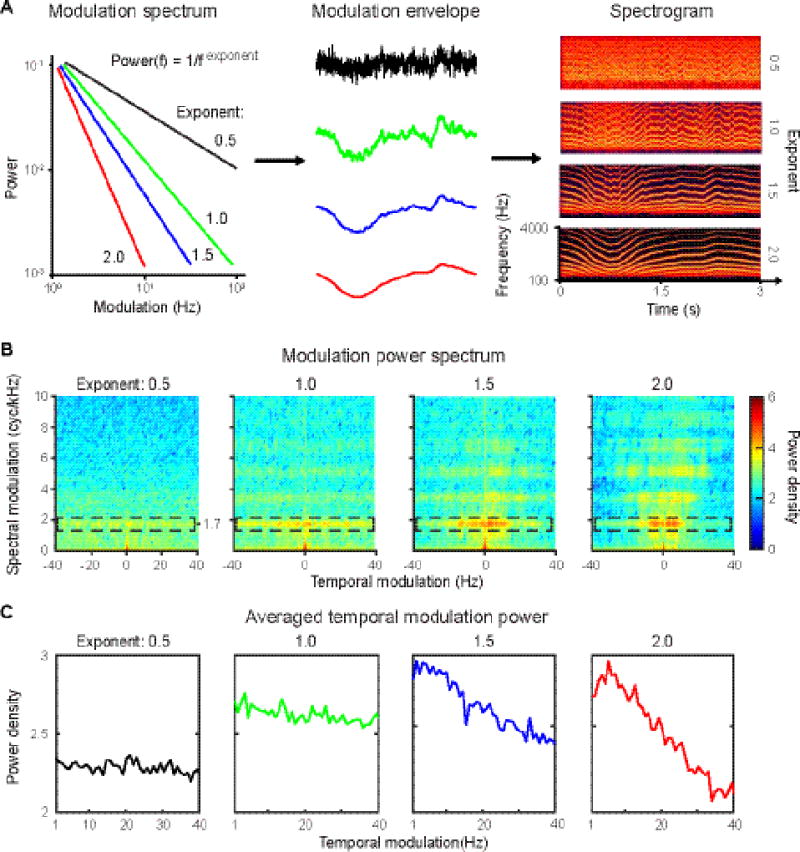
A, Schematic plot of stimulus generation. Left panel: schematic plot of modulation spectra used to generate modulation envelopes. The color code represents the spectra of different exponents. Black: 0.5; green: 1.0; blue: 1.5; red 2.0. Middle panel: modulation envelopes generated using the four different exponents. (Color code as in the modulation spectra.) Right panel: spectrograms of the four ‘frozen’ stimuli (see Methods) used in the experiment. Sound files of the stimuli can be accessed here: http://edmond.mpdl.mpg.de/imeji/collection/kZalRMtxa19mlRyG. B, Modulation power spectra of the four frozen stimuli. The dashed boxes show increased power density at a spectral modulation of around 1.7 cycles per 1000 Hz in the stimuli. C, The averaged temporal modulation spectrum. The averaged temporal modulation was computed by averaging along the spectral modulation dimension of the modulation power spectrum (in B). From left to right, the averaged temporal modulation spectrum of each stimulus becomes steeper as the exponent increases. Note that there are no prominent peaks in the averaged temporal modulation spectra that indicate regular modulations centered at a narrow frequency band.

We first generated spectral modulation envelopes with ‘random-walk’ profiles using an inverse Fourier method. We fit the modulation spectra to have a 1/f shape, with exponents at 0.5, 1, 1.5 and 2 (Fig. 1A left panel) and converted the spectra from the frequency domain back to the temporal domain using inverse Fourier transformation. The phase spectra were obtained from pseudo-random numbers drawn uniformly from the interval [0, 2π]. Because we fixed stimulus length to 3 seconds and the sampling rate to 44100 Hz, we created modulation spectra of 44100 * 3 points with a frequency range of 0 – 22050 Hz. Using different random number seeds for the phase spectra, we were able to generate spectral modulation envelopes (Fig.1A middle panel) with different dynamics for each exponent. The modulation envelopes were normalized to have unit standard deviation.

Second, we created tone complexes comprising tonal components spaced at third-octave intervals and then used the spectral modulation envelopes generated as above to modulate the tone complexes. We set the fundamental frequency to 200 Hz and limited the frequency range of the stimuli to between 200 Hz to 4000 Hz, well within humans’ sensitive hearing range. The frequencies of each tonal component were modulated through the frequency range from 200 Hz to 4 kHz by the envelopes generated in the first step. Modulated tonal components outside this frequency range at one end would re-enter it at the opposite end so that the number and spacing of the tonal components within this frequency range was always constant.

We used the same random seed to generate one stimulus for each of four exponents, 0.5, 1, 1.5, and 2, so that all four stimuli have the same phase spectrum but different modulation spectra. During the experiment, we presented these four stimuli 25 times, and we term these four the ‘frozen’ stimuli. Next, we used distinct random seeds to generate 25 ‘distinct’ stimuli with different phase spectra for each exponent. Each of these were presented once, creating four groups of ‘distinct’ stimuli. In total, there were eight stimulus groups, comprising four groups of ‘frozen’ stimuli and four groups of ‘distinct’ stimuli. In total, 200 stimuli (25 stimuli×4 exponents×2 stimulus types) were used in the study.

A 1000 Hz pure tone of 50 ms duration was inserted into the ‘distinct’ stimuli, and the onset of the tone was randomly distributed between 2.2 and 2.7 s. The signal-to-noise ratio of the tone to these distinct stimuli was fixed at −15 dB, because in preliminary testing we determined that a tone at SNR −15 dB can be detected at an adequate rate (i.e. avoiding ceiling or floor effects). We applied a cosine ramp-up function in a window of 30 ms at the onset of all stimuli and normalized the stimuli to ~70 dB SPL (sound pressure level).

Stimulus Analysis

To characterize the spectral and temporal modulations in our stimuli, we computed modulation power spectra (MPS) for the four ‘frozen’ stimuli used in the experiment (Fig. 1B) (Singh & Theunissen, 2003; Elliott & Theunissen, 2009). We first created time-frequency representations of the stimuli using the log amplitude of their spectrograms obtained with Gaussian windows. We then applied the 2D Fourier Transform to the spectrograms and created MPS by taking the amplitude squared as a function of the Fourier pairs of the time and frequency axes. As temporal modulations in our stimuli represent acoustic dynamics across timescales, we averaged the MPS across the spectral modulation dimension to show averaged temporal modulation spectra for each stimulus (Fig. 1C). Figure 1B shows that the prominent spectral modulation centers around 1.7 cycles per 1000 Hz; specifically, at this modulation frequency there is increased modulation power from exponent 0.5 to 2. Figure 1C shows that the averaged temporal modulations vary with the modulation spectra we used to generate each stimulus. The stimulus with exponent 0.5 shows a flat averaged temporal modulation spectrum and has low modulation power, whereas the stimulus with exponent 2.0 has the steepest averaged temporal modulation spectrum. Note, importantly, that the averaged temporal modulation spectra of all four stimuli show no peak of power density between 4 – 7 Hz (Fig. 1C).

MEG recording, preprocessing, and protocol

MEG signals were measured with participants in a supine position and in a magnetically shielded room using a 157-channel whole-head axial gradiometer system (KIT, Kanazawa Institute of Technology, Japan). A sampling rate of 1000 Hz was used, with an online 1–200 Hz analog band-pass filter and a notch filter centered around 60 Hz. After the main experiment, participants were presented with 1 kHz tone beeps of 50 ms duration as a localizer to determine their M100 evoked responses (Roberts et al., 2000). 20 channels with the largest M100 responses in both hemispheres (10 channels in each hemisphere) were selected as auditory channels for further analysis for each participant individually.

MEG data analysis was conducted in MATLAB 2015b (The MathWorks, Natick, MA) using the Fieldtrip toolbox 20160106 (Oostenveld et al., 2011) and the wavelet toolbox in MATLAB. Raw MEG data were noise-reduced offline using the time-shifted principle component analysis (de Cheveigné & Simon, 2007). Trials were visually inspected, and those with artifacts such as channel jumps and large fluctuations were discarded. An independent component analysis was then used to correct for artifacts caused by eye blinks, eye movements, heartbeat, and system noise. After preprocessing, 0 to (at most) 5 trials were removed for each exponent of each stimulus type, leaving a minimum of 20 trials per condition. To avoid biased estimation of inter-trial phase coherence, we included exactly 20 trials in the analysis for all exponents of all stimulus types. Each trial was divided into a 5 second epoch, with a 1 sec pre-stimulus period and a 4 sec post-stimulus period. Each trial was baseline corrected by subtracting the mean of the whole trial prior to further analysis.

During MEG scanning, all stimuli, both ‘frozen’ and ‘distinct’, were presented in a pseudo-randomized order for each participant. After each stimulus was presented, participants were required to push one of two buttons to indicate whether they heard a tone in the stimulus. Between 1–2s after participants responded, the next stimulus was presented. The participants were required to keep their eyes open and to fix on a white cross in the center of a black screen. The stimuli were delivered through plastic air tubes connected to foam ear pieces (E-A-R Tone Gold 3A Insert earphones, Aearo Technologies Auditory Systems).

Behavioral data analysis

Behavioral data were analyzed in MATLAB using the Palamedes toolbox 1.5.0 (Prins & Kingdom, 2009). For each exponent, there were 50 stimuli, half of which had a tone embedded. A two-by-two confusion matrix was created for each exponent by treating the trials with the tone embedded as ‘target’ and the other trials as ‘noise’. Correct detection of the tone in the ‘target’ trials was counted as ‘hit’, while reports of hearing a tone in the ‘noise’ trials were counted as ‘false alarm’; d-prime values were computed based on hit rates and false alarm rates of each table. A half artificial incorrect trial was added to the table with all correct trials (Macmillan & Creelman, 2004).

Evoked responses to tones

We calculated the root mean square (RMS) of evoked responses to the onset of tones for each ‘distinct’ group across 20 auditory channels and across 20 trials. Baseline was corrected using the MEG signal from 200-msec pre-onset of the tone in each selected channel. After baseline correction, we averaged RMS across 20 auditory channels.

Evoked responses to stimulus onset

We calculated RMS of evoked responses to the onset of stimulus for each ‘frozen’ group and each ‘distinct’ group across 20 auditory channels and across 20 trials. Baseline was corrected using the MEG signal from 200-msec pre-onset of the stimuli in each selected channel. After baseline correction, we averaged RMS across 20 auditory channels.

Local SNR of the embedded tones

The exponents of stimuli result in different modulation profiles and can modulate local SNR of the embedded tones across stimuli. Because the differences of local SNR could potentially explain the behavioral performance of tone detection, we computed the local SNR of the embedded tones using rectangular temporal windows combined with equivalent rectangular bandwidth (ERB) at 1000 Hz (Glasberg & Moore, 1990). We chose five temporal window sizes, 50, 100, 200, 300 and 500 ms, and five bandwidths, 0.25, 0.5, 1, 1.5, and 2 ERB (33, 66, 133, 199 and 265 Hz). Across different bandwidths, we centered the temporal window in the middle of the tone – 25 ms after tone onset – and computed power of the ‘distinct’ stimuli without the tone in this temporal window. Then, to compute local SNR, we divided the power of the tone by the power of the ‘distinct’ stimuli within the temporal window and the narrow band. We transformed the values of local SNR into decibels by taking a log with base 10 and multiplying by 10.

Phase coherence and power analysis

To extract time-frequency information, single-trial data from each MEG channel were transformed using functions of Morlet wavelets embedded in the Fieldtrip toolbox, with frequencies ranging from 1 to 50 Hz in steps of 1 Hz. As all the stimuli used are 3 seconds long, to be able to extract low frequency oscillations (e.g. 1 Hz) and to balance spectral and temporal resolution of time-frequency transformation, window length increased linearly from 1.5 cycles to 7 cycles from 1 to 20 Hz and then was kept constant at 7 cycles above 20 Hz. Phase and power responses were extracted from the wavelet transform output at each time-frequency point.

The ‘inter-trial phase coherence’ (ITPC) was calculated for all eight groups of stimuli at each time-frequency point (details can be seen in (Lachaux et al., 1999). ITPC is a measure of consistency of phase-locked neural activity entrained by a stimulus across trials. ITPC of a specific frequency band is thought to reflect cortical entrainment to temporal modulations in sounds (Luo et al., 2013; Ding & Simon, 2014; Doelling et al., 2014; Kayser et al., 2015) and therefore can be used as an index to indicate temporal coding of each stimulus type at certain frequency band here. Although event-evoked responses and ITPC both measure evoked neural responses and are highly correlated (Mazaheri & Picton, 2005), evoked responses show energy that spreads across a broad frequency range (VanRullen et al., 2014) and are limited by event rates (Lakatos et al., 2013). Furthermore, phase reset of ongoing oscillations of certain frequency band is not always correlated with sensory events (Mazaheri & Jensen, 2006; 2010). Therefore, we chose to use ITPC in our current study.

The induced power response was calculated for all eight groups of stimuli and was normalized by dividing the mean power value in the baseline range (−.6 ~ −.1 s) and converted to decibel units.

The ITPC and power response for four groups of ‘frozen’ stimuli were averaged from 0.25 s to 2.8 s post-stimulus to avoid effects of neural responses evoked by the stimulus onset and offset. We applied the same calculation of ITPC and power response to four groups of ‘distinct’ stimuli, but used the results as a baseline for the ITPC and power response of the ‘frozen’ stimuli. The differentiated ITPC (dITPC) and differentiated induced power were obtained by subtracting the ITPC and power response for ‘distinct’ stimuli out from ‘frozen’ stimuli for each participant. These two indices reflect phase-locked responses to the repeated temporal structure in the ‘frozen’ stimuli.

Auditory Processing model

The 1/f stimuli have a broadband modulation spectrum and contain information across all timescales. To quantify acoustic information on each timescale and later to examine on what timescale the auditory system groups acoustic information, we constructed an auditory processing model inspired by the concept of cochlear-scaled entropy (Stilp & Kluender, 2010; Stilp et al., 2010) using temporal filters of different sizes. By convolving temporal filters with the envelopes of the stimuli in each cochlear band, we can extract acoustic changes, which represent critical acoustic information on different timescales - and can be seen as an analogue to features in visual stimuli resulting from convolution with Gabor filters (Olshausen & Field, 2004). An illustration of this auditory processing model can be seen in Figure 4.

Figure 4. Illustration of the auditory processing model and differentiated mutual information results.

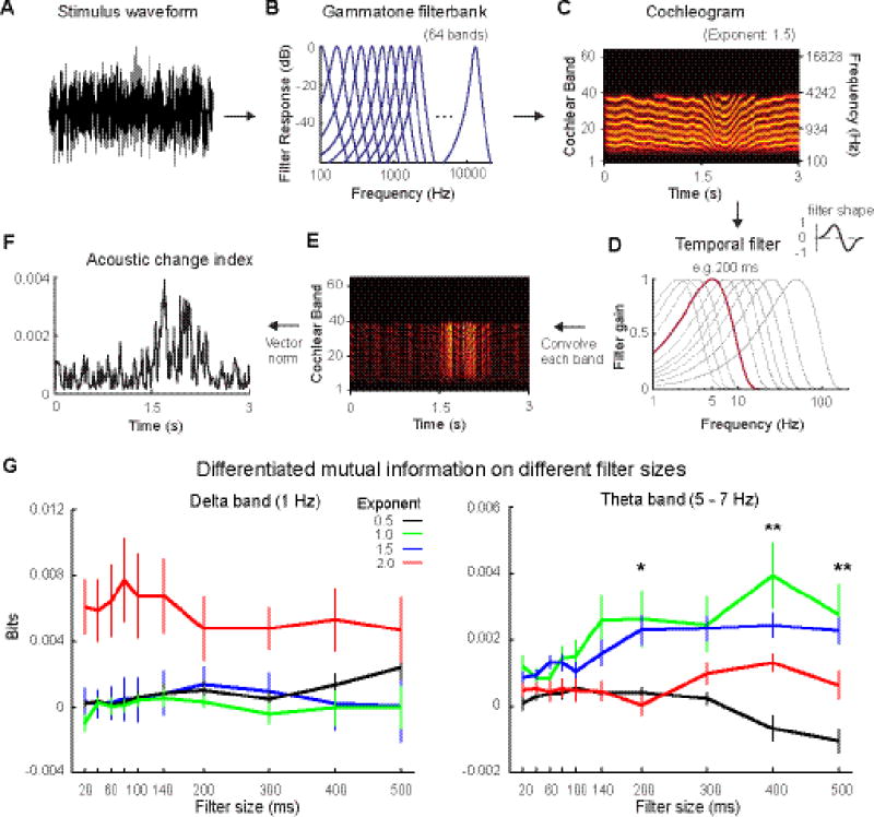
A, The waveform of a stimulus of exponent 1.5. B, A schematic plot of the Gammatone filter bank of 64 bands used in the model. C, The cochleogram of the stimulus. The left y-axis represents the number of the cochlear channels and the right y-axis represents the center frequency of each channel. D, Frequency responses of temporal filters. The frequency responses of all temporal filters were plotted. Beside the plot, the filter shape on temporal dimension is showed. We highlighted the frequency response of the temporal filter of 200 ms, which is used here for further illustrations. E, Convolution of the temporal filter with each band in the cochleogram. After convolving with the temporal filter, large values appear at time points where the modulation changes abruptly (depending on the temporal filter size). F, Acoustic change index (ACI) resulted from taking the vector norm of (E). G, Differentiated mutual information in the delta and theta bands across different filter sizes. X-axis: filter size of the temporal filter used in the auditory processing model. Y-axis: bits of differentiated mutual information. The color code is as in Figure 1. In the delta band, the differentiated mutual information does not vary with the filter size. Differentiated mutual information in the theta band varied with filter size (Asterisks indicate main effect of Exponent). The mutual information results demonstrate that the auditory processing model with temporal windows of > 200 ms is consistent with neural auditory processing extracting temporal regularities from irregular sounds. Lines and bars represent mean while error bars represent +/− SEM.

First, the stimuli were filtered using a gammatone filterbank of 64 bands. The envelope of each cochlear band was extracted by using Hilbert transformation on each band and taking the absolute values (Glasberg & Moore, 1990; Søndergaard & Majdak, 2013). We then convolved the envelope of each band with the temporal filters that we constructed (described below). The values calculated from the convolution were centered on the middle point of the temporal filters and were normalized according to the length of the temporal filter used. We padded 500 ms time points at the beginning and the end of the stimuli. After convolution, we took out padded points and only saved the time points of the original stimuli. We then took a vector norm at each time point across 64 cochlear bands.

The temporal filter was constructed by multiplying a Gaussian temporal window with one period of a sinusoid wave. We chose Gaussian temporal windows of ten sizes: 20, 40, 60, 80, 100, 140, 200, 300, 400, and 500 ms, with the mean centered in the middle of the temporal window and the standard deviation being one fifth of window length. We then created sinusoid waves from 0 to 2*pi with periods corresponding to each Gaussian temporal window. Then we multiplied one period of the sinusoid waves with 10 Gaussian temporal windows of corresponding sizes to create 10 temporal filters.

These temporal filters function as a one-dimensional filter that extracts changes in each cochlear band, which can be compared to narrowband spectral-temporal receptive fields often found in inferior colliculus (Escabí et al., 2003; Andoni et al., 2007; Carlson et al., 2012). Within a temporal window in which the envelope fluctuates abruptly, the output of the convolution would give a large value. The calculation of the vector norm summarizes temporal changes across all cochlear bands and generates a value at each time point that represents broadband spectro-temporal changes within this temporal window. This is intended to roughly correspond to auditory processes of cortical areas employing spectral-temporal receptive fields with broadband tuning properties (Theunissen et al., 2000; Machens et al., 2004; Theunissen & Elie, 2014). For example, if the frequency modulation changes abruptly and harmonics sweep across frequency bands within a temporal window, the convolution would generate large values that differ across frequency bands. Taking a vector norm would generate a high value. Therefore, we can quantify acoustic changes along both temporal and spectral domains using output from this model.

The model outputs calculated at each time point indicate the presence of acoustic changes on the timescale corresponding to the temporal filter size. We refer to the model outputs as Acoustic Change Index (ACI). Finally, we down-sampled the ACI from 44100 Hz to 100 Hz to match the sampling rate of the phase series in the MEG signals (100 Hz).

Differentiated mutual information between ACI and phase series

To determine at what timescale acoustic information is extracted by the auditory system, we computed mutual information between phase series of MEG signals and ACI. Mutual information is an index to quantify how much information is shared between two time series and suggests correlation between two series (Cogan & Poeppel, 2011; Gross et al., 2013; Ng et al., 2013; Kayser et al., 2015). We chose to compute mutual information instead of a linear correlation because ACI is an index of real numbers while the phase series is both circular and derived from imaginary numbers. A linear correlation cannot correctly measure the relationship between these two metrics. While ITPC cannot tell us which features in the stimulus drive robust phase coherence, if the phase series in the theta band is found to have high mutual information with ACI of this stimulus at a timescale of 200 ms, we can reasonably conclude that the auditory system extracts acoustic information in this stimulus on a timescale of 200 ms.

We computed the mutual information between the phase series of each frequency (1 – 50 Hz) collected under the frozen stimuli and ACI of different timescales for each corresponding ‘frozen’ stimulus type. Then we computed the mutual information between phase series collected under the ‘distinct’ stimuli and ACI of different timescales for each corresponding ‘frozen’ stimulus type. Next, we calculated the differences between the mutual information using trials collected under ‘frozen’ stimuli and the mutual information using trials under ‘distinct’ stimuli. By doing this, we subtracted out mutual information contributed by spontaneous phase responses evoked by sounds in general, and also normalized the mutual information across frequencies to remove the effects caused by 1/f characteristics of neural signals (He et al., 2010; He, 2014). This differentiated mutual information, resulted from using trials collected under ‘distinct’ stimuli as a baseline, highlighted the mutual information between the structure of ACI and the phase series of MEG signals. For example, we computed the mutual information between ACI for a frozen stimulus of exponent 1 and 20 phase series collected under this frozen stimulus from MEG signals, and then computed the mutual information between ACI for this frozen stimulus and 20 phase series collected from MEG signals when subjects were listening to 20 ‘distinct’ stimuli of exponent 1. We took a difference between these two values of mutual information and used this difference as the differentiated mutual information.

Mutual information was calculated with the Information Breakdown Toolbox in MATLAB (Pola et al., 2003; Magri et al., 2009). For each frequency of the MEG response, the phase distribution was composed of six equally spaced bins: 0 to pi/3, pi/3 to pi * 2/3, pi * 2/3 to pi, pi to pi * 4/3, pi * 4/3 to pi * 5/3, and pi * 5/3 to pi * 2. The ACI was grouped using 8 bins equally spaced from the minimum value to the maximum value. Eight bins were chosen to have enough discrete precision to capture changes in acoustic properties while making sure that each bin has sufficient counts for mutual information analysis, since the greater number of bins would lead to zero counts in certain bins.

The estimation of mutual information is subject to bias caused by finite sampling of the probability distributions because limited data was supplied in the present study. Therefore, a quadratic extrapolation embedded in the Information Breakdown Toolbox was applied to correct bias. Mutual information is computed on the data set of each condition. A quadratic function is then fit to the data points, and the actual mutual information is taken to be the zero-crossing value. This new value reflects the estimated mutual information for an infinite number of trials and greatly reduces the finite sampling bias (Montemurro et al., 2007; Panzeri et al., 2007). The mutual information value of each frequency was calculated for each subject and for each channel across trials before averaging.

Results

Tone detection performance increases with exponent though SNR is constant

Behavioral results

Subjects detected tones inserted into the ‘distinct’ stimuli. The behavioral results (Fig. 2A) demonstrate that participants’ sensitivity to tones (d-prime) increased to sounds with increasing exponent, although, importantly, the SNR is the same across all stimuli. The behavioral performance in detecting tones was examined using a repeated measures one-way ANOVA (rmANOVA) with the main factor of Exponent. There is a significant main effect of Exponent (F(3,42) = 34.07, p < 0.001, η_p² = .709), and a linear trend test showed a significant upward trend (F(1,14) = 59.19, p < 0.001, η_p² = .809).

Figure 2.

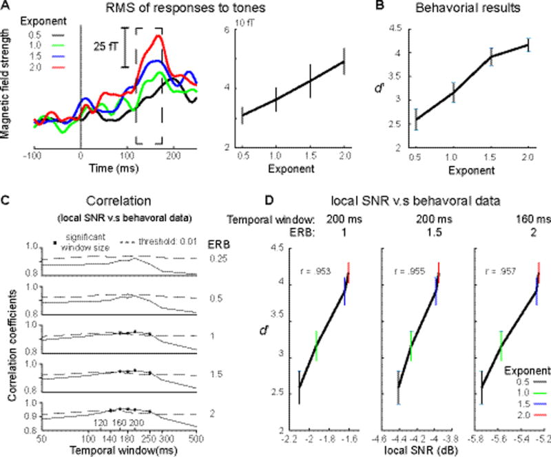
A, Root mean square (RMS) of MEG waveform responses to tones. Left panel: RMS of evoked fields to tones from 200 ms before tone onset to 250 ms after tone onset. (Color code as in Figure 1) The dashed box indicates the time range from 120 ms to 175 ms that show significant effects of the Exponent (p < 0.05, one-way rmANOVA). Right panel: RMS averaged from 120 ms to 175 ms. The behavioral and the RMS results show the same upward trend along exponent values. B, Behavioral results of tone detection. C, Correlations between tone detection performance and local SNR. ERB indicates bandwidth used to compute local SNR. ERB refers to one equivalent rectangular bandwidth (133 Hz) of the narrowband centered on 1000 Hz. Y axis indicates values of correlation coefficients. X axis shows different temporal window sizes. The dashed lines indicate significant thresholds (p < 0.01, one-sided) and the square highlights significant correlation results. Local SNRs computed using the temporal window ranging between 140 to 250 ms and the bandwidths larger than 1 ERB can explain the differences of tone detection rate across the different stimuli. D, local SNR plotted again behavioral data for the highest correlation of each bandwidth. From left to right, the bandwidth is 1, 1.5 and 2 ERB. Temporal window indicates the temporal window used to compute the high correlation of each bandwidth. X axis indicates local SNR. The color of error bars codes for different exponents. This result suggests that the auditory system uses a temporal window of ~ 200 ms to chunk the acoustic stream for separation of targets from background sounds. Lines represent mean, error bars represent +/− SEM.

RMS of Tone Evoked Responses

As the listeners’ performance on detecting tones varied across stimuli with different exponents of the 1/f stimuli, we examined whether the evoked responses elicited by the tones also show an effect of Exponent (Fig. 2B, upper panel). We calculated the RMS of the MEG signal elicited by tones, averaged over 20 auditory channels, and conducted, on each time point from the onset point of tones to 250 ms after tone onset, a one-way rmANOVA with Exponent as the main factor. After adjusted FDR correction, we found a significant main effect of Exponent from 120 ms to 175 ms (p < 0.01) after tone onset. To investigate this further, we averaged across this window and found a significant linear trend (F(1,14) = 25.16, p < 0.001, η_p² = .642). The result is shown in Figure 2B (lower panel). The RMS results correspond to behavioral results and demonstrate that exponents do modulate detection of tones. The behavioral results are not likely caused by response bias.

Local SNRs

The behavioral results and RMS results demonstrate that tone detection varies with exponent. Although the global SNR was matched across the stimuli with different exponents, local SNR varies with exponent and could cause differences of tone detection performance across different stimuli. Therefore, we computed local SNR using rectangular temporal windows of different sizes combined with ERBs of different bandwidths across all 25 trials for each of four exponents. The trial number marched the trails used in behavioral analysis. Pearson’s correlation between behavioral results and the local SNRs across four exponents was then calculated to assess whether the local SNR can explain tone detection performance.

We found high correlation coefficients (> 0.8) between behavioral results and local SNR computed using all combinations of temporal window sizes and ERB bandwidths (Fig. 2D). To rule out spurious correlations, we established a significant threshold by using a shuffling procedure. We first shuffled the labels of the four types of ‘distinct’ stimuli and generated a new set of stimuli, and then computed local SNR of each type of stimuli. We then correlated the local SNR with behavioral results to get a correlation coefficient for each combination of temporal window size and ERB bandwidth. We repeated this shuffling procedure 1000 times and used a right-sided alpha level of 99% as the significance threshold level. Significant correlations between behavioral results and local SNR were found for the temporal window sizes between 140 and 250 ms, combined with ERB bandwidths from 1 to 2. We plotted local SNR against tone detection performance on each exponent separately for the significant peak correlation computed using each ERB bandwidth (Fig. 2E). These results show that tone detection performance can be explained by the local SNR modulated by exponents. The acoustic structure of the stimuli becomes sparser with larger exponents and, therefore, local SNR increases, which facilitates tone detection in the stimuli. Most importantly, the local SNR computed using the temporal window of around 200 ms can best capture the behavioral variance. This suggests that a temporal window of ~ 200 ms is used by the auditory system to group acoustic information and extract salient changes in acoustic streams.

Exponent modulates onset responses and differentiated inter-trial phase coherence in the delta and theta bands

RMS of onset responses

As the acoustic structures of the 1/f stimuli vary with exponents, we examined whether the onset responses to the stimuli also show an effect of Exponent (Fig. 3A). We calculated the RMS of the MEG signal elicited by eight stimulus groups (four ‘frozen’ groups and four ‘distinct’ groups), averaged over 20 auditory channels, and conducted a one-way rmANOVA with Exponent as the main factor, separately for the ‘frozen’ stimuli and the ‘distinct’ stimuli. The one-way rmANOVA was conducted on each time point from the onset point to 250 ms after stimulus onset. After adjusted FDR correction, we found a significant main effect of Exponent for the ‘frozen’ stimuli from 90 ms to 115 ms and for the ‘distinct’ stimuli from 95 ms to 105 ms and from 115 ms to 130 ms (p < 0.01). The RMS results demonstrate that onset responses increase with exponents. As onset responses are sensitive to acoustic structures of sounds and are modulated by spectral complexity (Shahin et al., 2007), the results here are likely caused by the spectral sparsity – as the exponent increases, spectral modulation of the stimuli becomes more centered (Fig. 1) and, therefore, spectral sparsity increases with exponents.

Figure 3. RMS of responses to stimulus onset and differentiated inter-trial phase coherence (dITPC).

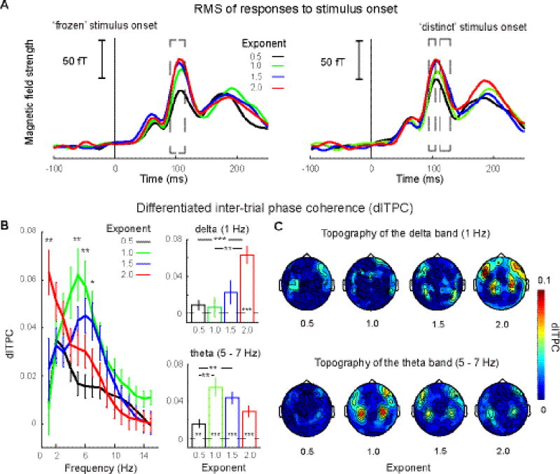
A, RMS of response to the ‘frozen’ and ‘distinct’ stimuli. Left panel: RMS of responses to the ‘frozen’ stimuli. Right panel: RMS of responses to the ‘distinct’ stimuli (color code as in Figure 1). The dashed box of the left panel indicates the time range from 90 ms to 115 ms that shows significant effects of the Exponent for the ‘frozen’ stimuli (p < 0.05, one-way rmANOVA). The dashed boxes of the right panel indicate the time ranges from 95 ms to 105 ms and from 115 ms to 130 ms that show significant effects of the Exponent for the ‘distinct’ stimuli. B, dITPC on auditory channels. Left panel: dITPC from 1 Hz to 15 Hz (color code as in Figure 1.) We found significant main effects of Exponent in two frequency bands: delta (1 Hz) and theta (5 – 7 Hz). Right panels: averaged dITPC within frequency bands. Asterisks inside bars indicate that dITPC is significantly above zero. The theta band activity tracks all stimuli, even if there is no regular temporal structure present; delta band activity is more narrowly responsive to stimuli with exponent 2. C, Topographies of dITPC in the delta and theta bands. Typical auditory response topographies can be seen in both bands. This underscores that the robust phase coherence results originate from auditory processing regions. Error bars represent +/− SEM.

Differentiated inter-trial phase coherence

The dITPC, the difference of phase coherence between the ‘frozen’ stimuli and the ‘distinct’ stimuli on the independently defined auditory channels, was calculated from 1 to 50 Hz. The results are shown in Figure 3B. We observed robust phase coherence in the theta band (5 – 7 Hz) for stimuli of all four exponents and some degree of selectivity for the stimuli with exponents 1 and 1.5. In the delta band (1 Hz) there was a preference in phase coherence for the stimuli with exponent 2. The topographies of dITPC for four exponents in the delta and theta bands are shown in Figure 3C.

To measure the effects of exponent on dITPC across frequencies, we conducted a one-way rmANOVA with Exponent as the main factor from 1 to 50 Hz. After adjusted FDR correction, this revealed a main effect of Exponent from 5 – 7 Hz (p < 0.05), which is in the theta band range, and a main effect at 1 Hz (p < 0.05), which is in the delta band. We then averaged dITPC within two frequency ranges separately and conducted a two-way rmANOVA with factors of Exponent and Frequency band (delta: 1 Hz; and theta: 5 – 7 Hz) on dITPC. We found a main effect of Exponent (F(3,42) = 5.24, p = 0.004, η_p² = .273) and an interaction between Exponent and Frequency band (Greenhouse-Geisser corrected: F(3,42) = 11.64, p < 0.001, η_p² = .454). A one-way rmANOVA with a factor of Exponent conducted separately for each frequency band shows a main effect both in the delta band (Greenhouse-Geisser corrected: F(3,42) = 7.69, p < 0.001, η_p² = .355) and in the theta band (F(3,42) = 8.28, p < 0.001, η_p² = .372). A post hoc paired t-test conducted in the theta band (5 – 7 Hz) showed that dITPC of stimuli with exponents 1 and 1.5 are significantly larger than the stimuli with exponent 0.5 (exponent 1: t(14) = 4.27, p = 0.006, d = 2.28; exponent 1.5: t(14) = 4.08, p = 0.006, d = 2.18) after Bonferroni correction. Comparison of dITPC for stimuli of exponents 1 and 1.5 with stimuli of exponent 2 were significant but did not survive correction for multiple comparisons (exponent 1: t(14) = 2.31, p = 0.036, d = 1.23; exponent 1.5: t(14) = 2.34, p = 0.035, d = 1.25). In the delta band (1 Hz), the paired t-test shown that dITPC of stimuli with exponent 2 is significantly larger than the stimuli with exponent 0.5 (t(14) = 7.12, p < 0.001, d = 3.81) and exponent 1.0 (t(14) = 4.16, p = 0.006, d = 2.22).

Because dITPC reflects the difference of phase coherence between the ‘frozen’ stimuli and the ‘distinct’ stimuli, a one-sample t-test against zero on dITPC of each stimulus type in each band tests whether there is robust phase-coherence across trials evoked by the ‘frozen’ stimuli. In the delta band (Fig. 3B, right upper panel), we found dITPC was significantly above zero when the exponent is 2 (t(14) = 6.80, p < 0.001, d = 3.63). In the theta band (Fig. 3B, right lower panel), we found significant dITPC above zeros across all exponents (Exponent 0.5: t(14) = 3.59, p = 0.024, d = 1.92; Exponent 1.0: t(14) = 5.45, p < 0.001, d = 2.91;Exponent 1.5: t(14) = 6.63, p < 0.001, d = 3.54; Exponent 2.0: t(14) = 4.64, p < 0.001, d = 2.48). Bonferroni correction was applied in each band.

In summary, the results show that all four types of ‘frozen’ stimuli evoked robust phase coherence in the theta band. This supports the hypothesis that phase coherence observed in the theta band (and in many studies) is not solely a result of stimulus driven entrainment, as no regular temporal modulation exists in the stimuli.

The stimuli with exponent 1 and 1.5 revealed higher phase coherence values than the stimuli with exponent 0.5. This phase coherence pattern in the theta band showed a similar pattern to findings in ferrets using single unit recording (Garcia-Lazaro et al., 2006). Our results further show that this coding preference comes from the theta band, which indicates an underlying auditory process on a timescale of ~150 ms – 250 ms. The auditory processing on a timescale of 150 – 250 ms, reflected by robust phase coherence in the theta band, may be critical and is possibly the reason for the preference found in Garcia-Lazaro et al (2006).

Surprisingly, we observed in the delta band that the stimuli of exponent 2 evoked robust phase coherence. The differences of dITPC patterns between the theta and delta bands indicate that the auditory system independently tunes to information on the timescales corresponding to the theta and delta bands (Cogan & Poeppel, 2011).

Differentiated Induced Power shows no effect

We examined effects of exponents on induced power from 1 to 50 Hz by conducting a one-way rmANOVA with Exponent as the main factor. We found no significant effect on Exponent from 1 to 50 Hz after adjusted FDR correction (p > 0.05). This suggests that the power response does not differentially code temporal information critically, which is also consistent with previous studies (Cogan & Poeppel, 2011; Luo & Poeppel, 2012; Ng et al., 2013; Doelling et al., 2014; Kayser et al., 2015).

Raw Power shows no effect and does not bias ITPC estimation

We examined effects of the exponents on raw power (without baseline correction) from 1 to 50 Hz by conducting a one-way rmANOVA with Exponent as the main factor. We did such tests on the ‘frozen’ stimuli and the ‘distinct’ stimuli, separately. We found no significant effect of Exponent for the ‘frozen’ stimuli from 1 to 50 Hz after adjusted FDR correction (p > 0.05). Similarly, we found no significant effect of Exponent for the ‘distinct’ stimuli from 1 to 50 Hz after adjusted FDR correction (p > 0.05). This suggests that the power is homogenous across different exponents and, therefore, estimation of ITPC for stimuli of different exponents should not be biased by the power.

Differentiated mutual information between phase and ACI on distinct scales

Next we used a mutual information approach to quantify at what timescale the acoustic information in the stimuli robustly entrained cortical oscillations in the delta (1 Hz) and theta (5 – 7 Hz) bands. In Figure 4A-F, we illustrate how ACI was generated by the auditory processing model. The waveforms of stimuli were filtered through the Gammatone filter bank of 64 bands (Fig. 4B) and cochleograms were generated for the ‘frozen’ stimuli (Fig. 4C). We convolved each band of the cochleogram with temporal filters of various lengths (Fig. 4D) and created a convovled cochleogram for each filter length (Fig. 4E). Vector norm was applied on the convolved cochleogram, which resulted in ACI. An example of ACI computed using a filter length of 200 ms was shown in Figure 4F. The ACI of each ‘frozen’ stimulus was used to compute mutual information. From the mutual information results, we found that the delta band oscillation was unaffected by the temporal filter size, whereas in the theta band the mutual information showed an effect of the filter size starting from 200 ms (Fig 4G).

A three-way Frequency band × Exponent × Filter size rmANOVA was conducted on differentiated mutual information. We found a significant main effect of Exponent (Greenhouse-Geisser corrected: F(4,42) = 5.22, p = 0.004, η_p² = .272). We also found significant interaction effects between Frequency band and Exponent (Greenhouse-Geisser corrected: F(3,42) = 8.42, p < 0.001, η_p² = .387), between Exponent and Filter size (F(27,378) = 1.58, p = 0.036, η_p² = .101), and between Frequency band and Exponent and Filter size (F(27,378) = 2.42, p < 0.001, η_p² = .147)

We then conducted a two-way Filter Size × Exponent rmANOVA in the delta band. We found a significant main effect of Exponent (Greenhouse-Geisser corrected: F(3,42) = 6.84, p = 0.007, η_p² = .328) but not of Filter size (Greenhouse-Geisser corrected: F(9,126) = .59, p = 0.802, η_p² = .041). The interaction was not significant (F(27,378) = 1.34, p = 0.123, η_p² = .087).

In the theta band, we conducted a two-way Filter Size × Exponent rmANOVA and found significant main effects of Exponent (Greenhouse-Geisser corrected: F(3,42) = 10.14, p < .001, η_p² = .420) and of Filter size (Greenhouse-Geisser corrected: F(9,126) = 7.19, p < .001, η_p² = .339). The interaction between Exponent and Filter size is also significant (F(27,378) = 5.10, p < .001, η_p² = .267). To test which filter size differentiates among stimulus types, we conducted a one-way rmANOVA on each filter size with Exponent as main factor. After Bonferroni correction, we found main effects of Exponent on the filter sizes: 200 ms (Greenhouse-Geisser corrected: F(3,42) = 7.69, p = .048, η_p² = .354), 400 ms (Greenhouse-Geisser corrected: F(3,42) = 12.74, p = .006, η_p² = .476) and 500 ms (Greenhouse-Geisser corrected: F(3,42) = 9.87, p = .010, η_p² = .414). Then, we examined what stimulus type was affected by filter size by conducting a one-way rmANOVA with Filter size as a main factor. We found a main effect on Filter size for the stimuli with exponent 0.5 (Greenhouse-Geisser corrected: F(9,126) = 6.82, p = .008, η_p² = .291), exponent 1.0 (Greenhouse-Geisser corrected: F(9,126) = 5.76, p = .036, η_p² = .328) and exponent 1.5 (Greenhouse-Geisser corrected: F(9,126) = 7.45, p < .001, η_p² = .347) but not for the stimuli with exponent 2 (F(9,126) = 2.22, p = .100, η_p² = .137).

To summarize the results of the differentiated mutual information analysis, we found that, although the stimuli in our experiment have a 1/f modulation spectrum and show no dominant temporal modulation frequencies or regular temporal patterns, the phase patterns of the theta band cortical oscillations were captured by the ACI extracting temporal information larger than 200 ms. On the other hand, cortical oscillations in the delta band are not captured by ACI computed on the timescales less than 500 ms.

The finding that the delta band is unaffected by the filter size is probably because the delta band oscillations tune to acoustic changes on a long timescale (e.g. > 1 s). The acoustic information represented by ACI is on a timescale smaller than 500 ms, which does not contribute to the global change of the stimuli extracted by a large temporal window (e.g. >1 s). Another explanation is that the delta band tunes to high-level information in the stimuli that our model fails to reveal.

That theta phase shows greater MI with ACI of timescales larger than 200 ms is consistent with the results of phase coherence in the theta band (Fig. 4). A reasonable hypothesis is that the auditory system uses a default temporal window of > 200 ms to chunk the continuous acoustic stream (VanRullen & Koch, 2003; Ghitza & Greenberg, 2009; Ghitza, 2012; Giraud & Poeppel, 2012; VanRullen, 2016). This temporal window size is reflected in the dominant theta oscillations found in both our results and in other studies (Ding & Simon, 2013; Luo et al., 2013; Andrillon et al., 2016). In stimuli without overt rhythmic structure, the auditory system actively parses the acoustic stream and extracts acoustic changes using a temporal window corresponding to roughly a cycle of a theta band oscillation. Because this chunking process has a limited time constant, i.e. 150 – 300 ms, only the acoustic changes on a timescale of larger than 200 ms are captured within acoustic dynamics across all timescales in our stimuli. Our auditory processing model using a temporal filter with different sizes simulated this hypothesized chunking process. The model used temporal windows to chunk acoustic streams and computed acoustic changes within each temporal window. The ACI on the timescale of ~ 200 ms, therefore, reflects the acoustic information extracted by this chunking process in the auditory system.

In summary, the results suggest that the auditory system uses a temporal windowing process to chunk acoustic information and extracts acoustic changes from irregular stimuli, and this temporal window is larger than 200 ms. The preference of the auditory system for stimuli with exponents 1 and 1.5, shown in our results in the theta band and in Garcia et al.(2006), is likely a result of this chunking process.

Discussion

We investigated neurophysiological responses to stimuli with 1/f modulation spectra and tested how listeners detect embedded tones. We found that cortical oscillations in the theta band track the irregular temporal structure and show a preference to 1/f stimuli with exponents 1 and 1.5, which roughly correspond to signals with the modulation spectrum of speech. The delta band oscillations are entrained by stimuli with exponent 2, which has the slowest temporal modulation. The fact that we find robust phase coherence in theta band in the absence of regular dynamics suggests that theta oscillations are not a simple consequence of the acoustic input but rather may represent the temporal structure of internal neural processing. By computing mutual information between the model outputs and the phase series in the delta and theta bands, we found that phase coherence in the theta band can be best explained by acoustic changes captured by temporal windows at least as large as 200 ms. Further supporting this finding, the local SNR computed using a temporal window of 200 ms predicts the tone detection rates and confirms the mechanism by which the auditory system uses a temporal window (~ 200 ms) to group acoustic information and extract salient acoustic changes.

Robust phase coherence in the theta band is not solely stimulus driven

Since the 1/f stimuli were not specifically modulated between 5 to 7 Hz to drive theta band oscillations (Fig. 1C), the robust theta oscillatory activity, therefore, must partly originate from an intrinsic auditory processing mechanism. In most of studies using rhythmic stimuli, the observed cortical entrainment in the theta band could be due to the fact that the regular temporal structure overlaps with the timescale of this architecturally intrinsic and probably innate grouping mechanism. Robust phase tracking in the theta band seems to be ubiquitously evoked by sounds. It has been shown, for example, that repeated noise induces phase coherence in the theta band, and the magnitude of phase coherence correlates with behavioral performance (Luo et al., 2013; Andrillon et al., 2016). In such studies, there is no regular temporal structure in sounds centered in the theta band that entrains the theta band oscillations.

One reason for theta band tracking of sounds of various temporal structures, regular and irregular, is possibly that the theta band oscillations play an active role in perceptual grouping of acoustic information, rather than being passive, stimulus driven neural activities (Ghitza & Greenberg, 2009; Schroeder et al., 2010; Ghitza, 2012; Riecke et al., 2015). Our auditory processing model simulates this chunking process across timescales, and the mutual information results between the model outputs and phase series in the theta band differentiate stimuli of different exponents on a timescale larger than 200 ms and echoes the results of dITPC. Therefore, the robust phase coherence can be explained by the chunking process simulated by our auditory processing model (Fig. 4A-F).

The active chunking process is probably a trade-off between integrating a long period of acoustic information for precise analysis and making timely perceptual decisions. Although acoustic streams are continuous, the auditory system cannot integrate acoustic information over an arbitrary long period because of limited information capacity of the auditory system and of requirements for humans to make fast perceptual decisions. This chunking process of ~ 200 ms divides continuous acoustic streams into discrete perceptual units, so that further auditory analysis could be conducted timely within a ~ 200 ms temporal window for humans to make immediate perceptual decisions.

Preferential tuning to exponents 1 and 1.5 due to chunking

Our results of dITPC in the theta band indicate a preference of the auditory system for stimuli with exponents 1 and 1.5, which replicate the response pattern found in Garcia et al. (2006) using single unit recording in ferret primate auditory cortex. Furthermore, the mutual information results (Fig. 4) suggest that this preference is likely caused by the chunking process with temporal windows larger than 200 ms in the auditory system. Although all of the 1/f stimuli have dynamics across all timescales, the chunking process mainly extracts dynamics on a timescale corresponding to the theta band. The stimuli with exponents less than 1 and larger than 1.5 are either modulated too rapidly or too slowly, so that the dynamics on the timescale of the theta band range has less ‘chunking potency’ than in the stimuli with exponents 1 and 1.5.

Tone detection results explained by local SNR confirms a chunking process of ~200 ms

We found that although the long-term SNR of tones is the same across all four types of stimuli, the detection rates differ because of local SNR modulated by the exponents. These results are illuminated by the informational masking literature, which suggests that the structure of background sounds (maskers) matters when listeners try to detect a target (Brungart, 2001; Kidd et al., 2007). The key finding here is that participant behavior is modulated by the structure of background maskers in the same 200 ms window. This suggests the auditory system is extracting 200 ms windows for temporal analysis. This finding supports our interpretation of the neural data, discussed above, that the auditory system groups acoustic information on a timescale of ~ 200 ms and further suggests that this chunking process is probably fundamental for further auditory analysis. That is to say, the separation of targets from background sounds is probably built on this chunking process.

Delta band oscillations are invariant to acoustic details on timescales less than 500 ms

We found that only the stimuli with exponent 2 evoked robust phase coherence in the delta band, which supplements the findings by Garcia et al. (2006). The mutual information results in the delta band do not vary with the filter sizes used in the auditory processing model. This surprising result further suggests that the delta band oscillations are probably not sensitive to low-level acoustic details, but probably to a high-level perceptual cues, such as linguistic structure in speech (Ding et al., 2015), and attention-related rhythmic processing (Lakatos et al., 2008; Schroeder et al., 2010).

Memory and attention as potential confounds

As the ‘frozen’ stimuli were repeatedly presented to the participants while each of the ‘distinct’ stimuli was only presented once, one might surmise that the participants are able to memorize the ‘frozen’ stimuli. Previous studies have shown, though, that it is challenging, and perhaps even impossible, for humans to memorize acoustic local details of sounds textures of more than 200 ms long (McDermott et al., 2013; Teng et al., 2016), well short of the 3-second length of our stimuli. (Obviously, speech or music can be encoded and recalled.) As the ‘frozen’ and the ‘distinct’ stimuli were comparable in terms of long-term acoustic properties, such as spectral modulation and spectrum, the participants had to remember the acoustic details to be able to tell apart the ‘frozen’ stimuli from the ‘distinct’ stimuli with corresponding exponents. It would be very challenging indeed for the participants to differentiate one ‘frozen’ stimulus out of 25 ‘distinct’ stimuli with similar long-term acoustic properties. If the participants could successfully identify each ‘frozen’ stimulus, we would not expect memory to be affected by the exponent of frequency modulation, as we have found here. Therefore, we conjecture that memory does not contribute significantly to our results.

With regard to attention, as we only presented the target tones in the ‘distinct’ stimuli, so it would be possible that the participants could choose to only attend to the distinct stimuli to detect the tone. If the participants could distinguish the ‘frozen’ and ‘distinct’ stimuli by memorizing the ‘frozen’ stimuli and figure out that tones are contained only in each of the distinct stimuli (we did not tell the participants this information), we would expect that the tone detection performance should be similar across all exponents, as the participants could simply choose the ‘distinct’ stimuli as the target. But we did find a difference of tone detection across different exponents and this difference, importantly, can be explained by our acoustic analysis on local SNRs (Fig. 2).

Therefore, although it is true that memory and attention are always relevant considerations, the effects caused by memory and attention are unlikely to form the explanatory basis of our main results.

Conclusion: active chunking on a timescale of ~ 200 ms in the auditory system

Our results demonstrate an active chunking scheme in the auditory system (Poeppel, 2003; Ghitza & Greenberg, 2009; Panzeri et al., 2010; Ghitza, 2012; Giraud & Poeppel, 2012; VanRullen, 2016): on the timescale of ~ 200 ms, the auditory system actively groups acoustic information to parse a continuous acoustic stream into segments. The robust phase coherence in the theta band is not solely driven by external stimuli but also reflects active chunking. This chunking scheme is prevalent in auditory processing of sounds of various dynamics and may serve as a fundamental step for further perceptual analysis.

Abbreviations

MEG

magnetoencephalography

dB

decibel

SPL

sound pressure level

MPS

modulation power spectra

RMS

root mean square

SNR

Signal to noise ratio

ERB

equivalent rectangular bandwidth

ITPC

Inter-trial phase coherence

dITPC

differentiated ITPC

ACI

acoustic change index

MI

mutual information

References

- Andoni S, Li N, Pollak GD. Spectrotemporal receptive fields in the inferior colliculus revealing selectivity for spectral motion in conspecific vocalizations. Journal of Neuroscience. 2007;27:4882–4893. doi: 10.1523/JNEUROSCI.4342-06.2007. [DOI] [PMC free article] [PubMed] [Google Scholar]
- Andrillon T, Kouider S, Agus T, Pressnitzer D. Perceptual Learning of Acoustic Noise Generates Memory-Evoked Potentials. Curr Biol. 2016;25:2823–2829. doi: 10.1016/j.cub.2015.09.027. [DOI] [PubMed] [Google Scholar]
- Brungart DS. Informational and energetic masking effects in the perception of two simultaneous talkers. J Acoust Soc Am. 2001;109:1101–1109. doi: 10.1121/1.1345696. [DOI] [PubMed] [Google Scholar]
- Carlson NL, Ming VL, Deweese MR. Sparse Codes for Speech Predict Spectrotemporal Receptive Fields in the Inferior Colliculus. PLoS Comput Biol. 2012;8:1–15. doi: 10.1371/journal.pcbi.1002594. [DOI] [PMC free article] [PubMed] [Google Scholar]
- Cogan GB, Poeppel D. A mutual information analysis of neural coding of speech by low-frequency MEG phase information. J Neurophysiol. 2011;106:554–563. doi: 10.1152/jn.00075.2011. [DOI] [PMC free article] [PubMed] [Google Scholar]
- de Cheveigné A, Simon JZ. Denoising based on time-shift PCA. J Neurosci Meth. 2007;165:297–305. doi: 10.1016/j.jneumeth.2007.06.003. [DOI] [PMC free article] [PubMed] [Google Scholar]
- Ding N, Simon JZ. Adaptive Temporal Encoding Leads to a Background-Insensitive Cortical Representation of Speech. J Neurosci. 2013;33:5728–5735. doi: 10.1523/JNEUROSCI.5297-12.2013. [DOI] [PMC free article] [PubMed] [Google Scholar]
- Ding N, Simon JZ. Cortical entrainment to continuous speech: functional roles and interpretations. Front. Hum. Neurosci. 2014;8:1–7. doi: 10.3389/fnhum.2014.00311. [DOI] [PMC free article] [PubMed] [Google Scholar]
- Ding N, Melloni L, Zhang H, Tian X, Poeppel D. Cortical tracking of hierarchical linguistic structures in connected speech. Nat Neurosci. 2015;19:158–164. doi: 10.1038/nn.4186. [DOI] [PMC free article] [PubMed] [Google Scholar]
- Doelling KB, Poeppel D. Cortical entrainment to music and its modulation by expertise. Proc. Natl. Acad. Sci. U. S. A. 2015;112:E6233–E6242. doi: 10.1073/pnas.1508431112. [DOI] [PMC free article] [PubMed] [Google Scholar]
- Doelling KB, Arnal LH, Ghitza O, Poeppel D. Acoustic landmarks drive delta–theta oscillations to enable speech comprehension by facilitating perceptual parsing. NeuroImage. 2014;85(Part 2 IS):761–768. doi: 10.1016/j.neuroimage.2013.06.035. [DOI] [PMC free article] [PubMed] [Google Scholar]
- Elliott TM, Theunissen FE. The Modulation Transfer Function for Speech Intelligibility. PLoS Comput Biol. 2009;5:1–14. doi: 10.1371/journal.pcbi.1000302. [DOI] [PMC free article] [PubMed] [Google Scholar]
- Escabí MA, Miller LM, Read HL, Schreiner CE. Naturalistic Auditory Contrast Improves Spectrotemporal Coding in the Cat Inferior Colliculus. J Neurosci. 2003;23:11489–11504. doi: 10.1523/JNEUROSCI.23-37-11489.2003. [DOI] [PMC free article] [PubMed] [Google Scholar]
- Garcia-Lazaro JA, Ahmed B, Schnupp JWH. Tuning to Natural Stimulus Dynamics in Primary Auditory Cortex. Curr Biol. 2006;16:264–271. doi: 10.1016/j.cub.2005.12.013. [DOI] [PubMed] [Google Scholar]
- Ghitza O. On the role of theta-driven syllabic parsing in decoding speech: intelligibility of speech with a manipulated modulation spectrum. Front Psychol. 2012 doi: 10.3389/fpsyg.2012.00238. [DOI] [PMC free article] [PubMed] [Google Scholar]
- Ghitza O, Greenberg S. On the Possible Role of Brain Rhythms in Speech Perception: Intelligibility of Time-Compressed Speech with Periodic and Aperiodic Insertions of Silence. Phonetica. 2009;66:113–126. doi: 10.1159/000208934. [DOI] [PubMed] [Google Scholar]
- Giraud A-L, Poeppel D. Cortical oscillations and speech processing: emerging computational principles and operations. Nat Neurosci. 2012;15:511–517. doi: 10.1038/nn.3063. [DOI] [PMC free article] [PubMed] [Google Scholar]
- Glasberg BR, Moore BCJ. Derivation of auditory filter shapes from notched-noise data. Hear Res. 1990;47:103–138. doi: 10.1016/0378-5955(90)90170-t. [DOI] [PubMed] [Google Scholar]
- Gross J, Hoogenboom N, Thut G, Schyns P, Panzeri S, Belin P, Garrod S. Speech rhythms and multiplexed oscillatory sensory coding in the human brain. PLoS Biol. 2013;11:e1001752. doi: 10.1371/journal.pbio.1001752. [DOI] [PMC free article] [PubMed] [Google Scholar]
- He BJ. Scale-free brain activity: past, present, and future. Trends Cogn Sci. 2014:1–8. doi: 10.1016/j.tics.2014.04.003. [DOI] [PMC free article] [PubMed] [Google Scholar]
- He BJ, Zempel JM, Snyder AZ, Raichle ME. The Temporal Structures and Functional Significance of Scale-free Brain Activity. Neuron. 2010;66:353–369. doi: 10.1016/j.neuron.2010.04.020. [DOI] [PMC free article] [PubMed] [Google Scholar]
- Henry MJ, Obleser J. Frequency modulation entrains slow neural oscillations and optimizes human listening behavior. Proc. Natl. Acad. Sci. U. S. A. 2012;109:20095–20100. doi: 10.1073/pnas.1213390109. [DOI] [PMC free article] [PubMed] [Google Scholar]
- Henry MJ, Herrmann B, Obleser J. Entrained neural oscillations in multiple frequency bands comodulate behavior. Proc. Natl. Acad. Sci. U. S. A. 2014;111:14935–14940. doi: 10.1073/pnas.1408741111. [DOI] [PMC free article] [PubMed] [Google Scholar]
- Herrmann B, Henry MJ, Grigutsch M, Obleser J. Oscillatory Phase Dynamics in Neural Entrainment Underpin Illusory Percepts of Time. J Neurosci. 2013;33:15799–15809. doi: 10.1523/JNEUROSCI.1434-13.2013. [DOI] [PMC free article] [PubMed] [Google Scholar]
- Kayser SJ, Ince RAA, Gross J, Kayser C. Irregular Speech Rate Dissociates Auditory Cortical Entrainment, Evoked Responses, and Frontal Alpha. Journal of Neuroscience. 2015;35:14691–14701. doi: 10.1523/JNEUROSCI.2243-15.2015. [DOI] [PMC free article] [PubMed] [Google Scholar]
- Kerlin JR, Shahin AJ, Miller LM. Attentional gain control of ongoing cortical speech representations in a "cocktail party". Journal of Neuroscience. 2010;30:620–628. doi: 10.1523/JNEUROSCI.3631-09.2010. [DOI] [PMC free article] [PubMed] [Google Scholar]
- Kidd G, Jr, Mason CR, Richards VM, Gallun FJ, Durlach NI. Informational Masking. In: Yost WA, Popper AN, Fay RR, editors. Auditory Perception of Sound Sources, Springer Handbook of Auditory Research. Springer US; Boston, MA: 2007. pp. 143–189. [Google Scholar]
- Lachaux J-P, Rodriguez E, Martinerie J, Varela FJ. Measuring phase synchrony in brain signals. Hum. Brain Mapp. 1999;8:194–208. doi: 10.1002/(SICI)1097-0193(1999)8:4<194::AID-HBM4>3.0.CO;2-C. [DOI] [PMC free article] [PubMed] [Google Scholar]
- Lakatos P, Karmos G, Mehta AD, Ulbert I, Schroeder CE. Entrainment of Neuronal Oscillations as a Mechanism of Attentional Selection. Science. 2008;320:110–113. doi: 10.1126/science.1154735. [DOI] [PubMed] [Google Scholar]
- Lakatos P, Musacchia G, O’Connel MN, Falchier AY, Javitt DC, Schroeder CE. The spectrotemporal filter mechanism of auditory selective attention. Neuron. 2013;77:750–761. doi: 10.1016/j.neuron.2012.11.034. [DOI] [PMC free article] [PubMed] [Google Scholar]
- Luo H, Poeppel D. Phase patterns of neuronal responses reliably discriminate speech in human auditory cortex. Neuron. 2007;54:1001–1010. doi: 10.1016/j.neuron.2007.06.004. [DOI] [PMC free article] [PubMed] [Google Scholar]
- Luo H, Poeppel D. Cortical oscillations in auditory perception and speech: evidence for two temporal windows in human auditory cortex. Front Psychol. 2012;3:170. doi: 10.3389/fpsyg.2012.00170. [DOI] [PMC free article] [PubMed] [Google Scholar]
- Luo H, Tian X, Song K, Zhou K, Poeppel D. Neural Response Phase Tracks How Listeners Learn New Acoustic Representations. Curr Biol. 2013;23:968–974. doi: 10.1016/j.cub.2013.04.031. [DOI] [PubMed] [Google Scholar]
- Machens CK, Wehr MS, Zador AM. Linearity of Cortical Receptive Fields Measured with Natural Sounds. J Neurosci. 2004;24:1089–1100. doi: 10.1523/JNEUROSCI.4445-03.2004. [DOI] [PMC free article] [PubMed] [Google Scholar]
- Macmillan NA, Creelman CD. Detection Theory. Psychology Press; 2004. [Google Scholar]
- Magri C, Whittingstall K, Singh V, Logothetis NK, Panzeri S. A toolbox for the fast information analysis of multiple-site LFP, EEG and spike train recordings. BMC Neurosci. 2009;10:81. doi: 10.1186/1471-2202-10-81. [DOI] [PMC free article] [PubMed] [Google Scholar]
- Mazaheri A, Jensen O. Posterior α activity is not phase-reset by visual stimuli. Proc. Natl. Acad. Sci. U. S. A. 2006;103:2948–2952. doi: 10.1073/pnas.0505785103. [DOI] [PMC free article] [PubMed] [Google Scholar]
- Mazaheri A, Jensen O. Rhythmic pulsing: linking ongoing brain activity with evoked responses. Front. Hum. Neurosci. 2010;4 doi: 10.3389/fnhum.2010.00177. [DOI] [PMC free article] [PubMed] [Google Scholar]
- Mazaheri A, Picton TW. EEG spectral dynamics during discrimination of auditory and visual targets. Cognitive Brain Res. 2005;24:81–96. doi: 10.1016/j.cogbrainres.2004.12.013. [DOI] [PubMed] [Google Scholar]
- McDermott JH, Schemitsch M, Simoncelli EP. Summary statistics in auditory perception. Nat Neurosci. 2013;16:493–498. doi: 10.1038/nn.3347. [DOI] [PMC free article] [PubMed] [Google Scholar]
- Montemurro MA, Senatore R, Panzeri S. Tight data-robust bounds to mutual information combining shuffling and model selection techniques. Neural Comput. 2007;19:2913–2957. doi: 10.1162/neco.2007.19.11.2913. [DOI] [PubMed] [Google Scholar]
- Ng BSW, Logothetis NK, Kayser C. EEG phase patterns reflect the selectivity of neural firing. Cereb. Cortex. 2013;23:389–398. doi: 10.1093/cercor/bhs031. [DOI] [PubMed] [Google Scholar]
- Oldfield RC. The assessment and analysis of handedness: The Edinburgh inventory. Neuropsychologia. 1971;9:97–113. doi: 10.1016/0028-3932(71)90067-4. [DOI] [PubMed] [Google Scholar]
- Olshausen BA, Field DJ. Sparse coding of sensory inputs. Curr Opin Neurobiol. 2004;14:481–487. doi: 10.1016/j.conb.2004.07.007. [DOI] [PubMed] [Google Scholar]
- Oostenveld R, Fries P, Maris E, Schoffelen J-M. Fieldtrip: open source software for advanced analysis of MEG, EEG, and invasive electrophysiological data. Comput Intell Neurosci. 2011;2011:1–9. doi: 10.1155/2011/156869. [DOI] [PMC free article] [PubMed] [Google Scholar]
- Panzeri S, Brunel N, Logothetis NK, Kayser C. Sensory neural codes using multiplexed temporal scales. Trends Neurosci. 2010;33:111–120. doi: 10.1016/j.tins.2009.12.001. [DOI] [PubMed] [Google Scholar]
- Panzeri S, Senatore R, Montemurro MA, Petersen RS. Correcting for the Sampling Bias Problem in Spike Train Information Measures. J Neurophysiol. 2007;98:1064–1072. doi: 10.1152/jn.00559.2007. [DOI] [PubMed] [Google Scholar]
- Peelle JE, Gross J, Davis MH. Phase-locked responses to speech in human auditory cortex are enhanced during comprehension. Cerebral Cortex. 2013;23:1378–1387. doi: 10.1093/cercor/bhs118. [DOI] [PMC free article] [PubMed] [Google Scholar]
- Poeppel D. The analysis of speech in different temporal integration windows: cerebral lateralization as “asymmetric sampling in time”. Speech Commun. 2003;41:245–255. [Google Scholar]
- Pola G, Thiele A, Hoffmann KP, Panzeri S. An exact method to quantify the information transmitted by different mechanisms of correlational coding. Network. 2003;14:35–60. doi: 10.1088/0954-898x/14/1/303. [DOI] [PubMed] [Google Scholar]
- Prins N, Kingdom FAA. Palamedes: Matlab routines for analyzing psychophysical data. 2009 http://www.palamedestoolbox.org.
- Riecke L, Sack AT, Schroeder CE. Endogenous Delta/Theta Sound-Brain Phase Entrainment Accelerates the Buildup of Auditory Streaming. Curr Biol. 2015;25:3196–3201. doi: 10.1016/j.cub.2015.10.045. [DOI] [PubMed] [Google Scholar]
- Roberts TP, Ferrari P, Stufflebeam SM, Poeppel D. Latency of the auditory evoked neuromagnetic field components: stimulus dependence and insights toward perception. J Clin Neurophysiol. 2000;17:114–129. doi: 10.1097/00004691-200003000-00002. [DOI] [PubMed] [Google Scholar]
- Schroeder CE, Wilson DA, Radman T, Scharfman H, Lakatos P. Dynamics of Active Sensing and perceptual selection. Curr Opin Neurobiol. 2010;20:172–176. doi: 10.1016/j.conb.2010.02.010. [DOI] [PMC free article] [PubMed] [Google Scholar]
- Shahin AJ, Roberts LE, Miller LM, McDonald KL, Alain C. Sensitivity of EEG and MEG to the N1 and P2 Auditory Evoked Responses Modulated by Spectral Complexity of Sounds. Brain Topogr. 2007;20:55–61. doi: 10.1007/s10548-007-0031-4. [DOI] [PMC free article] [PubMed] [Google Scholar]
- Singh NC, Theunissen FE. Modulation spectra of natural sounds and ethological theories of auditory processing. J Acoust Soc Am. 2003;114:3394–3411. doi: 10.1121/1.1624067. [DOI] [PubMed] [Google Scholar]
- Stilp CE, Kluender KR. Cochlea-scaled entropy, not consonants, vowels, or time, best predicts speech intelligibility. Proc. Natl. Acad. Sci. U. S. A. 2010;107:12387–12392. doi: 10.1073/pnas.0913625107. [DOI] [PMC free article] [PubMed] [Google Scholar]
- Stilp CE, Kiefte M, Alexander JM, Kluender KR. Cochlea-scaled spectral entropy predicts rate-invariant intelligibility of temporally distorted sentencesa) J Acoust Soc Am. 2010;128:2112–2126. doi: 10.1121/1.3483719. [DOI] [PMC free article] [PubMed] [Google Scholar]
- Søndergaard PL, Majdak P. The Auditory Modeling Toolbox. In: Blauert J, editor. The Technology of Binaural Listening. Springer Berlin Heidelberg; Berlin, Heidelberg: 2013. pp. 33–56. [Google Scholar]
- Teng X, Tian X, Poeppel D. Testing multi-scale processing in the auditory system. Scientific Reports. 2016;6 doi: 10.1038/srep34390. 34390EP–. [DOI] [PMC free article] [PubMed] [Google Scholar]
- Theunissen FE, Elie JE. Neural processing of natural sounds. Nat Rev Neurosci. 2014;15:355–366. doi: 10.1038/nrn3731. [DOI] [PubMed] [Google Scholar]
- Theunissen FE, Sen K, Doupe AJ. Spectral-temporal receptive fields of nonlinear auditory neurons obtained using natural sounds. J Neurosci. 2000;20:2315–2331. doi: 10.1523/JNEUROSCI.20-06-02315.2000. [DOI] [PMC free article] [PubMed] [Google Scholar]
- VanRullen R. Perceptual Cycles. Trends Cogn Sci. 2016:1–13. doi: 10.1016/j.tics.2016.07.006. [DOI] [PubMed] [Google Scholar]
- VanRullen R, Koch C. Is perception discrete or continuous? Trends Cogn Sci. 2003;7:207–213. doi: 10.1016/s1364-6613(03)00095-0. [DOI] [PubMed] [Google Scholar]
- VanRullen R, Zoefel B, Ilhan BA. On the cyclic nature of perception in vision versus audition. Philos Trans R Soc Lond B Biol Sci. 2014;369:20130214–20130214. doi: 10.1098/rstb.2013.0214. [DOI] [PMC free article] [PubMed] [Google Scholar]
- Voss RF, Clarke J. ’’1/f noise’’ in music: Music from 1/f noise. J Acoust Soc Am. 1978;63:258–263. [Google Scholar]
- Zion Golumbic EM, Ding N, Bickel S, Lakatos P, Schevon CA, McKhann GM, Goodman RR, Emerson RG, Mehta AD, Simon JZ, Poeppel D, Schroeder CE. Mechanisms Underlying Selective Neuronal Tracking of Attended Speech at a “Cocktail Party”. Neuron. 2013;77:980–991. doi: 10.1016/j.neuron.2012.12.037. [DOI] [PMC free article] [PubMed] [Google Scholar]