Self-organization across scales: from molecules to organisms

Abstract

Creating ordered structures from chaotic environments is at the core of biological processes at the subcellular, cellular and organismic level. In this perspective, we explore the physical as well as biological features of two prominent concepts driving self-organization, namely phase transition and reaction–diffusion, before closing with a discussion on open questions and future challenges associated with studying self-organizing systems.

This article is part of the theme issue ‘Self-organization in cell biology’.

1. Introduction

A frequently used definition for self-organization is the dynamic emergence of order from the collective behaviour of individual agents [1]. As a consequence, self-organization can occur at various length and time scales. From non-equilibrium thermodynamics [2], it has been known for a long time that a system kept off equilibrium can self-organize by forming oscillations, chemical waves and stationary patterns [3–5]. Intriguingly, a living organism, fuelled by ATP and GTP hydrolysis, can also be considered a system far from equilibrium [6–8]. On the following pages, we will separately discuss the principles driving self-organization in biological systems, focusing mainly on phase transition and reaction–diffusion. For both concepts, we will first introduce the principles underlying self-organization from a physical perspective, before discussing biological examples on the molecular, cellular and organismal level. We will then reflect on the benefits of such self-organizing structures within a living system, before closing with open questions and future challenges.

2. Phase transition: from disordered to ordered state

(a). Phase transition from the physical perspective

Phase transition describes the ability of a physical system to switch between different states, resulting in the change of the overall collective behaviour or some intrinsic property of the whole system. To introduce the underlying principle, we would like to start with a small thought experiment. Let us assume a system composed of identical elements that diffuse, fuelled by Brownian motion, freely through the medium. Following the rules of classical statistical mechanics, in a completely random environment composed of identical elements the probability for every possible combination is equal. Thus, the probability of having such a system in state x is

where Z is the partition function of the system, E is the energy of the system in state x, and β is the thermodynamic parameter. For simplicity, we rescale the system so β = 1. To characterize the order of a system, generally an order-parameter, such as a pattern that emerges due to spatial constraints among individual elements, is used. Now in terms of the order parameter s_o, determined by the number of ordered micro-states N_o, we have

Analogously, s_do is determined by the number of disordered micro-states N_do

Considering no changes in temperature and constants rescaled to 1, we can put

where

and similarly

Intuitively, one would assume that bringing constraints into a system should lower the probability of occurrence, as the number of options is restricted by a specific set of rules. Thus, and . This, however, means that if then. Hence, from a statistical perspective it is more probable to end up with a disorganized state than an organized state of the system. The apparent question arising from this line of thought is why self-organization should emerge in the first place. Theoretically, this could be achieved by turning to , which can be achieved by introducing interaction potentials. Alternatively, one could also change to , by defining the interacting potentials as dominant compared with random fluctuations and collisions.

(i). Example 1—density and phase transition

In the following, we present one example of how an ordered, self-organized system may emerge. As above, we consider a dissipative system composed of an infinite number of identical elements A. So we have

where A_o refers to an ordered system following a particular spatio-temporal pattern that can be expressed by an analytical function. A_do represents the disordered state containing a random pattern or distribution. At steady state, we thus have

where k_o and k_do represent the rate constants towards their respective states. Under steady-state condition the system will fluctuate between the ordered and disordered states, whereby the overall state at a given point in time will be the linear combination of all possible states. So we have

whereby

Now let us include a coulombic-type interaction with enthalpy of reaction and ) and k_do proportional to thermal noise in the system. For simplicity, we further assume that thermal noise as well as G_do, which represents entropy without internal bonding, remains constant. Next, we slowly increase the density of elements in the system. In an initial scenario, no internal interactions exist owing to super-low density of A (figure 1a, top panel in blue). We thus have , and . This intuitively makes sense, since the probability of creating order in a noisy system in the absence of interaction is very unlikely. Next, let us assume we slightly increase internal interactions by elevating the density of A (figure 1a, top panel in green). Specifically, we decrease , thereby increasing the interacting force to the point that . Under these conditions, we obtain and . On first sight, this appears counterintuitive, as ordered and disordered phase are equal in energy. However, as the order parameter follows and , the relation is satisfied when since . Thus, at steady state the system will fluctuate with equal probabilities between ordered and disordered phases. Finally, we strongly increase density, thus maximizing interaction potential, so that (figure 1a, top panel in yellow). This will decrease , causing with and . Under these conditions, the system will arrest itself in the organized state.

Figure 1.

Self-organization across scales via density-dependent phase transitions. (a) Energy profiles depicting phase transition under various densities (top) and upon introduction of nonlinear interactions (bottom). (b) Density-dependent phase transitions in sliding actin filaments. Tracks (top) and directionality (middle) of rhodamine-labelled actin filaments plated on immobilized myosin at low concentration (left panels) and high concentration (right panels), respectively. At the bottom, density-dependent alignment (indicated by Kuiper statistic (KS) score) is plotted as function of actin filament length. (c) Density-dependent phase transitions in collective migration of keratinocytes. Cells were plated at 1.8 (top, left), 5.3 (top, middle) and 14.7 (top, right) cells/10 000 µm². Tracing cell migration (middle panels) as well as analysis of order parameter (bottom) both show a density-dependent transition from random to collective cell migration. (d) Density-dependent phase transitions in fish school behaviour. Typical configurations in fish school include swarm state, polarized state and milling. Below, phase transition for individual fish densities are plotted based on polarization and rotation of individual animals within groups. Images were obtained from (b) [9], (c) [10] and (d) [11].

(ii). Example 2—phase transition in dissipative systems

As illustrated in Example 1, phase-transition can be achieved by altering the density of A. However, the energy profiles are static for a given conditions. How then can a dynamic, self-organizing system emerge without changing external parameters? This can be achieved by introducing nonlinearity into the system. In our second example, we will do so by including a second agent B (figure 1a, bottom), where , and the positive number n defines the strength of the feedback loop. We now can write

For simplicity, we assume that and , while , which means that the entropy of the disordered state does not change significantly with introduction of matter into the system. Making it a function of time, we can rewrite the equation as

As the disorganized system absorbs free agent B (figure 1a, bottom panel in blue), new B enters the system from the connected reservoir. The resulting increase in [B(t)] leads to decrease in and elevates , thereby creating a positive feedback loop. Consequentially, the system transitions into an organized state (figure 1a, bottom panel in yellow), thereby recapitulating the phenomena of self-organization of a dissipative system away from thermodynamic equilibrium.

(b). Phase transition from the biological perspective

Phase transition for proteins in solution was described over 40 years ago [12]. Since then, it has been established that proteins in solution can form crystals and polymers as well as gels and dense liquids [13]. Here, the main contributors to the free energy (i.e. enthalpy) of the phase transition are water structures at the molecular surface [14] and protein properties such as surface charges [15]. Likewise, phase separation is an important concept for the organization of lipids [16] and proteins [17] within membranes. Intriguingly, recent work suggests that phase transitions also occur at the cellular level, where for instance liquid states have been observed for P-bodies [18], nucleoli [19] and stress granules [20]. Intriguingly, phase transition and phase separation were also described to play a relevant role on the multicellular level, where differences in the strength of adhesion between various cell types can lead to pattern formation [21], or collective cell rearrangements [22,23]. Considering that phase transition of molecules and cells is the focus of several perspectives in this issue, we refer readers interested in learning more on this topic to these essays as well as to other reviews on this exciting subject [14,24].

Phase transitions have also been observed to coordinate movement of individual agents. Experiments based on self-propelled particles, where vibration is used to create motion of macroscopic objects, showed that contact and shape are sufficient to elicit collective behaviour [25,26]. Likewise, density-dependent phase transition can also be observed with actin filaments in vitro [9]. Using a two-dimensional motility assay with immobilized myosin, on top of which actin filaments can move, showed self-organization that manifested as parallel alignment of actin filaments in a density-dependent manner (figure 1b). Notably, filament gliding takes up a preferred orientation at densities found in living cells, while orientation extends over length scales similar to the size of mammalian cells. Density-dependent phase transition can also be observed at the level of collective cell movement. For instance, transition from disorganized to organized state was observed for moving fish keratinocytes (figure 1c) [10]. Importantly, independent theoretical work based on an escape and capture model argues that density-dependent phase transition in collective cell migration does not correlate to cell–cell interaction strength [27]. Finally, phase transition can also be observed at the organismic level. Here, phase transitions occur in response to changes in population size or density (figure 1d) in fish [11], ants [28] and locusts [29]. Furthermore, changes in the behaviour of individuals within a swarm are sufficient to trigger phase transition, for instance during flash expansion in the case of predator exposure [30]. This is relevant, as it suggests that swarms transition stimulus-dependently between various collective states [31], thus creating complex decentralized input–output relations. However, determining accurately the physical energy of such complex systems is not always feasible. Thus, some phenomena, in particular in multicellular systems, may better be considered as a kind of phase transition using conceptual energy. For readers interested in this topic, we refer to excellent reviews published elsewhere [32,33].

3. Reaction–diffusion mechanisms

(a). Reaction–diffusion from the physical perspective

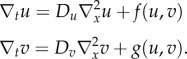
Fuelled by Brownian motion, each chemical reaction is subject to diffusion. Intriguingly, under particular conditions, reaction–diffusion systems can form complex patterns out of chaotic initial conditions. In this section, we will develop the basic idea behind reaction–diffusion systems. The simplest equation of a reaction–diffusion system is the one-component system with one single reaction and diffusion term

where u represents the concentration, D is the diffusion rate and R(u) is the reaction term. One requirement for creating spatio-temporal patterns in a one-component system is a wave-like solution. So looking for the above equation for travelling wave solutions of the form

yields

where c is the propagation speed of the wave, x represents the spatial coordinate and t the time. Converting this second-order differential equation into two first-order differential equations, we have

Before we further proceed with the theory, let us first introduce some terms that will be used in the following section.

Phase portrait: Every nonlinear dynamic system can be represented by the rate of change of its state variables in a phase portrait. For example, a one-component dynamic system can be represented as a two-dimensional coordinate system, where one axis depicts the state variable and the other axis represents the rate of change of the state variable. The resulting vector field trajectories of the phase portrait indicate how a particular system will evolve.

Critical points: These are points in the phase portrait that represent static positions in a dynamical system. In other words, these are the equilibrium points of the system, where the rate of change of the state variables is zero. Critical points come in three types that differ from each other as follows. Stable point/attractors are equilibrium points towards which, upon small perturbation, the dynamic system converges back in the phase portrait. In other words, the rate vectors around this point are directed towards it. Upon linearization, the sign of the rate along the eigendirection is towards the critical point, which is indicated by a negative eigenvalue. In contrast to stable points, the system diverges away from an unstable point in the phase portrait upon small perturbation. In this case, the rate vectors point away from that critical point. Similarly, upon linearization, the eigenvalues are positive. Finally, saddle points are neither local maxima nor local minima. Upon a small perturbation, the system will evolve to a particular direction unlike the case of a stable or unstable point. Importantly, a dynamical system can be linearized around those critical points.

Having established the basics, let us now return to the theory. Intuitively, we can think of the two first-order differential equations described before as a damped system, with c analogous to the drag coefficient and D analogous to the mass. Just for convenience, let us say , so the system can be described as

Considering that reaction–diffusion systems are nonlinear in nature, in the sense that the state variables of the system have nonlinear dependencies represented by and , we need to linearize the above problem around the critical points via Taylor expansion. Taking only the linear term, we have

For convenience, we take

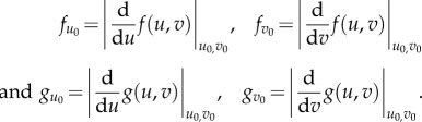So, near the critical point for small perturbation, we have

where 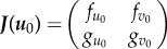is the Jacobian matrix. The nature of eigenvalues determines the trajectories of the above linear system around its critical point. As already mentioned above, in the case of a stable point the eigenvalues are negative, for an unstable point the eigenvalues are positive, and assuming a two-dimensional case, for a saddle one eigenvalue is positive and the other one is negative. Thus, the sum of eigenvalues is always negative for stable points, positive for unstable points, and either positive or negative for saddle points. If we now look into the product of the eigenvalues, then stable and unstable points are both positive, while saddle points are negative. Importantly, for a linear system, the sum and the product of eigenvalues are given by the trace and the determinant of the Jacobian matrix, respectively. Thus, as we linearized the system, the nature of the critical points can be determined simply by looking into the trace and determinant of the Jacobian.

(i). Example 1—one-component systems

Let us assume a monostable case such as Fisher's equation [34]

Here, the critical points are and , and the corresponding Jacobians are and 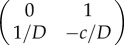. So looking at the trace and determinant of the Jacobian at each critical point indicates that u₊ is a stable fixed point with a negative sign, while u₀ is a saddle. What does that mean? To better understand the nature of the system, let us consider its phase portrait diagram as a landscape, wherein the curves depicting the potential represent the contours of a hill. Now, we can place a ball on that landscape, such that its position represents the position of the wave u(x − ct) in u space. Thus, by looking at the potential landscape, it is intuitive that the ball will for the monostable case roll towards the stable point where u = 0. Physically, this means that with time the wave invades space with lower u (figure 2a).

Figure 2.

Self-organization across scales via reaction–diffusion mechanisms. (a) One-component reaction–diffusion simulations of monostable (a) and bistable (a′) examples. (a) To the left, scheme of the potential landscape (i.e. V(u)) for propagating waves in monostable one-component case. Using the rolling ball analogy, the direction of the propagation of the wave can be determined (red arrow). Here, the ball rolls into the potential well, indicating that the wave will propagate in the direction of lower u or where u = 0. In the middle, the state variable u at time t = 0 is shown. The arrows indicate the direction of propagation of the wave, indicating invasion of space with lower u. To the right, temporal wave evolution is shown. (a′) Scheme of potential landscape (i.e. V(u)) for bistable one-component case with fixed points corresponding to u = 0, 1 and 2. Using the rolling ball analogy, we can see that the two balls will roll into the potential well u = 1 (red arrow). In the middle, again the state variable u at time t = 0 is shown. In this case, we have the sum of two waves analogous to the two balls in the left figure. Here, the arrows indicate the direction of propagation, indicating that the waves invade space with u = 1. To the right, temporal wave evolution is shown. (b) Simulations of reaction–diffusion systems starting with random noise. From the left to the right, systems were computed containing single-component monostable (R(u) =−u(u − 1)), single-component bistable (R(u) = −(u − 1)(u − 2)), and two-component activator–inhibitor (f(u, v) = c₁*u²/v − c₂*u and g(u,v) = c₃*u² − c₄*v). Starting from random noise, the plots depict the propagation of individual reactions through time. Note that two components are required for the formation of stable organized patterns in the presence of diffusion (code for simulation is provided in the supplementary material). (c) Arrangement of cilia in hair cells. At the top, scanning electron micrograph (SEM) of hair bundle (left) and freeze–fracture SEM (right) from the apical surface of a bullfrog hair cell. Below, blue and red lines (left) depict gradient distribution used to compute hair cell pattern (right). (d) Growth-dependent rearrangement of stripe pattern in the fish Pomacanthus imperator. Below, stripe pattern of fish (left) and simulation (right) are shown. (e) Emergence of fairy circles in arid grassland based on biomass–water feedback. At the top, aerial view of fairy circles formed by spinifex grass in Australia. Below, examples of real fairy circles (left) and from simulations (right) are shown. Images were obtained from (c) [35], (d) [36] and (e) [37].

Next, let us observe the system under bistable conditions such as

Here, the critical points are and the corresponding Jacobians are and . Here, trace and determinant of the Jacobians indicate that u₋ and u₊ are saddle fixed points while u₀ is the stable fixed point. Again, employing the ‘rolling ball analogy’, we consider the landscape derived from phase portrait. In this case, waves will propagate from the two saddle points representing two state values to the minima/stable fixed point u = 1. Physically, this means that waves with amplitude greater than 1 will move towards regions with offset 1, and waves with amplitude less than 1 will also move to amplitude 1. Thus, at infinite time, simple patterns emerge (figure 2a′). However, it should be noted that the system will not necessarily end up in two coexisting states, but may under certain initial conditions form only one state.

In summary, reaction–diffusion systems containing only one component can form either homogeneous or transient inhomogeneous random patterns. However, formation of dynamical complex patterns in one-component reaction–diffusion systems is unlikely.

(ii). Example 2—two-component systems

Turing first stated that in the presence of stochastic noise a two-component reaction–diffusion system may form a long-lived pattern, a finding that 20 years later was rediscovered by Gierer & Meinhardt [38,39]. In the following, we will explore the necessary condition for the formation of such patterns. A two-component reaction–diffusion system in its simplest form can be written as

Or, we can also write the equations together as

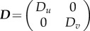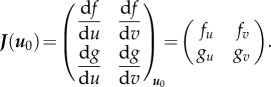
where , and 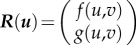. As we are interested in the equilibrium points u₀, we will solely look at the linear dependence close to equilibrium. So we can consider R(u) as . As J(u) is the Jacobian, it can also be written as the first-order linear dependency matrix

Next, let us consider a small plane wave perturbation such that . Here, diffusion near the static, homogeneous equilibrium leads to the new linear dependency matrix given by

Considering , the instability condition for the onset of plane wave/front generation is given by

Together, the first two conditions explain the stability condition of an equilibrium point in the absence of diffusion terms. Under the given conditions, the eigenvalues are negative, and so the sum of eigenvalues is negative and their product is positive. By contrast, the last condition introduces linear instability into the system with the help of diffusion. Here, appropriate selection of diffusion coefficients for u and v will result in the onset of bifurcation, which will trigger the generation of fronts/waves required for pattern formation. The instability brought by the linear diffusion in the locally stable equilibria can then be used to form a stable limit cycle, which leads unlike the monostable and bistable case to formation of oscillations in the system and thus to the formation of complex spatio-temporal patterns (figure 2b). At the bifurcation or critical point , we have the critical wave number, which leads to specific wave patterns depending on the type of diffusion coefficients satisfying the conditions below with

and so the spectrum of plane waves satisfying the instability condition

will lead to the formation of waves or linear combination of them and thus complex patterns. The system following the above set of constraints is often coined an activator–inhibitor system.

(b). Reaction–diffusion from the biological perspective

Components required for self-organization via reaction–diffusion are ubiquitous in cells. For instance, simple diffusion waves and/or gradients have been put forward, for example, for lipids and calcium in migrating cells [40,41], or Cdc42 during yeast budding [42]. Likewise, basic reaction types, such as ultrasensitivity [43], bistablity [44] and oscillators [45], are readily available in nature. Not surprisingly, reaction–diffusion systems, as introduced by Turing and later by Gierer & Meinhardt [38,39], were proposed to control cellular features (figure 2c) such as cell shape [46] and cell polarization [47] as well as cell migration [48]. As on the single cell level, two-component reaction–diffusion mechanisms were suggested to contribute to tissue organization (figure 2d), including limb development [49,50] and digit patterning [51], as well as pigmentation of skin [52,53]. Intriguingly, patterns similar to Turing-type patterns were even discussed on the organismal level (figure 2e) [37]. However, it should be noted that different molecular mechanisms can yield surprisingly similar patterns. For instance, self-organization reminiscent of Turing-type patterns can be generated by differential adhesion without resorting to reaction–diffusion processes [21]. Another example is the Min complex, where a pole-to-pole oscillation is used to determine spatial information within the cell [54]. Not surprisingly, more recent models have challenged the validity of previously published reaction–diffusion models (e.g. [55,56] versus [57]). Collectively, these data argue that a plethora of mechanisms are employed for self-organization across scales in space and time. As above, we recommend to the interested reader excellent reviews on this evolving topic [58,59].

4. Future challenges

Self-organization is a physico-chemical phenomenon of great importance for the formation of functional units at the cellular, tissue and organismic level. However, despite substantial advancements in recent years, we are still far from a comprehensive view.

In this perspective, we have focused on two distinct concepts driving self-organization—phenomena based on phase transition and models based on reaction–diffusion. While the physical principles driving phase transition and reaction–diffusion were introduced separately, we would like to note that these reactions are by no means independent from each other. For instance, considering that phase separation may alter diffusion rates as well as concentration of individual molecules, it is plausible to envision that a specific reaction–diffusion system may differ in different phases within the same cell. Future experiments will show whether individual reaction–diffusion systems based on the same components may coexist within the same cell and/or whether induced transition of individual molecules between phases may act as a signal analogous to phosphorylation.

How could a better understanding of the underlying principles be harnessed to advance life science? Recent work has established that misguided self-organization via errors in phase transition [60,61] or reaction–diffusion [51] are medically relevant. It would thus be interesting to revisit some disease models from such a perspective. Furthermore, it would also be intriguing to explore self-organization in synthetic systems [62]. Synthetic biology aims at both constructing biological systems bottom-up and redesigning biological systems to perform novel tasks [63,64]. As such, it provides the unique possibility to study the relevance of self-organization uncoupled from co-occurring events present in biological systems. Indeed, such studies have already yielded essential insights on the principles of self-organization (e.g. microtubules [65,66], contractile FtsZ rings [67]) and self-production (e.g. autopoiesis of micelles [68,69]) of subcellular structures. Considering the rapid advancement of synthetic biology, self-organizing principles emerging from these studies may provide features critical to structure and stabilize future, increasingly complex artificial systems.

Data accessibility

This article has no additional data.

Authors' contributions

T.S. and M.G. prepared the images and wrote the perspective together.

Competing interests

The authors declare no competing interests.

Funding

This work was supported by funds from the German research foundation to T.S. and M.G. (DFG EXC-1003).

References

- 1.Karsenti E. 2008. Self-organization in cell biology: a brief history. Nat. Rev. Mol. Cell Biol. 9, 255–262. ( 10.1038/nrm2357) [DOI] [PubMed] [Google Scholar]
- 2.Groot SD, Mazur P. 1984. Non-equilibrium thermodynamics. New York, NY: Dover Publications. [Google Scholar]
- 3.Briggs TS, Rauscher WC. 1973. An oscillating iodine clock. J. Chem. Educ. 50, 496 ( 10.1021/ed050p496) [DOI] [Google Scholar]
- 4.Epstein IR, Pojman JA, Steinbock O. 2006. Introduction: self-organization in nonequilibrium chemical systems. Chaos 16, 37101 ( 10.1063/1.2354477) [DOI] [PubMed] [Google Scholar]
- 5.De Kepper P, Epstein IR, Kustin K. 1981. Bistability in the oxidation of arsenite by iodate in a stirred flow reactor. J. Am. Chem. Soc. 103, 6121–6127. ( 10.1021/ja00410a023) [DOI] [Google Scholar]
- 6.Ornes S. 2017. Core concept: how nonequilibrium thermodynamics speaks to the mystery of life. Proc. Natl Acad. Sci. USA 114, 423–424. ( 10.1073/pnas.1620001114) [DOI] [PMC free article] [PubMed] [Google Scholar]
- 7.Hernández-Lemus E. 2012. Nonequilibrium thermodynamics of cell signaling. J. Thermodyn. 2012, 1–10. ( 10.1155/2012/432143) [DOI] [Google Scholar]
- 8.Ahsendorf T, Wong F, Eils R, Gunawardena J. 2014. A framework for modelling gene regulation which accommodates non-equilibrium mechanisms. BMC Biol. 12, 102 ( 10.1186/s12915-014-0102-4) [DOI] [PMC free article] [PubMed] [Google Scholar]
- 9.Butt T, Mufti T, Humayun A, Rosenthal PB, Khan S, Khan S, Molloy JE. 2010. Myosin motors drive long range alignment of actin filaments. J. Biol. Chem. 285, 4964–4974. ( 10.1074/jbc.M109.044792) [DOI] [PMC free article] [PubMed] [Google Scholar]
- 10.Szabo B, Szollosi GJ, Gonci B, Juranyi Z, Selmeczi D, Vicsek T. 2006. Phase transition in the collective migration of tissue cells: experiment and model. Phys. Rev. E Stat. Nonlin. Soft Matter Phys. 74, 61908 ( 10.1103/PhysRevE.74.061908) [DOI] [PubMed] [Google Scholar]
- 11.Tunstrøm K, Katz Y, Ioannou CC, Huepe C, Lutz MJ, Couzin ID. 2013. Collective states, multistability and transitional behavior in schooling fish. PLoS Comput. Biol. 9, e1002915 ( 10.1371/journal.pcbi.1002915) [DOI] [PMC free article] [PubMed] [Google Scholar]
- 12.Tanaka T, Ishimoto C, Chylack L. 1977. Phase separation of a protein-water mixture in cold cataract in the young rat lens. Science 197, 1010–1012. ( 10.1126/science.887936) [DOI] [PubMed] [Google Scholar]
- 13.Vekilov PG. 2012. Phase diagrams and kinetics of phase transitions in protein solutions. J. Phys. Condens. Matter 24, 193101 ( 10.1088/0953-8984/24/19/193101) [DOI] [PubMed] [Google Scholar]
- 14.Vekilov PG. 2010. Phase transitions of folded proteins. Soft Matter 6, 5254 ( 10.1039/c0sm00215a) [DOI] [Google Scholar]
- 15.Li P, et al. 2012. Phase transitions in the assembly of multivalent signalling proteins. Nature 483, 336–340. ( 10.1038/nature10879) [DOI] [PMC free article] [PubMed] [Google Scholar]
- 16.Heberle FA, Feigenson GW. 2011. Phase separation in lipid membranes. Cold Spring Harb. Perspect. Biol. 3, a004630 ( 10.1101/cshperspect.a004630) [DOI] [PMC free article] [PubMed] [Google Scholar]
- 17.Banjade S, Rosen MK. 2014. Phase transitions of multivalent proteins can promote clustering of membrane receptors. eLife 3, e04123 ( 10.7554/eLife.04123) [DOI] [PMC free article] [PubMed] [Google Scholar]
- 18.Brangwynne CP, Eckmann CR, Courson DS, Rybarska A, Hoege C, Gharakhani J, Jülicher F, Hyman AA. 2009. Germline P granules are liquid droplets that localize by controlled dissolution/condensation. Science 324, 1729–1732. ( 10.1126/science.1172046) [DOI] [PubMed] [Google Scholar]
- 19.Brangwynne CP, Mitchison TJ, Hyman AA. 2011. Active liquid-like behavior of nucleoli determines their size and shape in Xenopus laevis oocytes. Proc. Natl Acad. Sci. USA 108, 4334–4339. ( 10.1073/pnas.1017150108) [DOI] [PMC free article] [PubMed] [Google Scholar]
- 20.Wippich F, Bodenmiller B, Trajkovska MG, Wanka S, Aebersold R, Pelkmans L. 2013. Dual specificity kinase DYRK3 couples stress granule condensation/dissolution to mTORC1 signaling. Cell 152, 791–805. ( 10.1016/j.cell.2013.01.033) [DOI] [PubMed] [Google Scholar]
- 21.Bonforti A, Duran-Nebreda S, Montañez R, Solé R. 2016. Spatial self-organization in hybrid models of multicellular adhesion. Chaos 26, 103113 ( 10.1063/1.4965992) [DOI] [PubMed] [Google Scholar]
- 22.Beaune G, et al. 2014. How cells flow in the spreading of cellular aggregates. Proc. Natl Acad. Sci. USA 111, 8055–8060. ( 10.1073/pnas.1323788111) [DOI] [PMC free article] [PubMed] [Google Scholar]
- 23.Steinberg MS. 1963. Reconstruction of tissues by dissociated cells. Some morphogenetic tissue movements and the sorting out of embryonic cells may have a common explanation. Science 141, 401–408. ( 10.1126/science.141.3579.401) [DOI] [PubMed] [Google Scholar]
- 24.Heisenberg C-P. 2017. D'Arcy Thompson's ‘on growth and form’: from soap bubbles to tissue self-organization. Mech. Dev. 145, 32–37. ( 10.1016/j.mod.2017.03.006) [DOI] [PubMed] [Google Scholar]
- 25.Kudrolli A. 2010. Concentration dependent diffusion of self-propelled rods. Phys. Rev. Lett. 104, 88001 ( 10.1103/PhysRevLett.104.088001) [DOI] [PubMed] [Google Scholar]
- 26.Deseigne J, Dauchot O, Chate H. 2010. Collective motion of vibrated polar disks. Phys. Rev. Lett. 105, 98001 ( 10.1103/PhysRevLett.105.098001) [DOI] [PubMed] [Google Scholar]
- 27.Romanczuk P, Couzin ID, Schimansky-Geier L. 2009. Collective motion due to individual escape and pursuit response. Phys. Rev. Lett. 102, 10602 ( 10.1103/PhysRevLett.102.010602) [DOI] [PubMed] [Google Scholar]
- 28.Beekman M, Sumpter DJ, Ratnieks FL. 2001. Phase transition between disordered and ordered foraging in Pharaoh's ants. Proc. Natl Acad. Sci. USA 98, 9703–9706. ( 10.1073/pnas.161285298) [DOI] [PMC free article] [PubMed] [Google Scholar]
- 29.Buhl J, Sumpter DJT, Couzin ID, Hale JJ, Despland E, Miller ER, Simpson SJ. 2006. From disorder to order in marching locusts. Science 312, 1402–1406. ( 10.1126/science.1125142) [DOI] [PubMed] [Google Scholar]
- 30.Pitcher TJ, Parrish JK. 1993. Functions of shoaling behaviour in teleosts. In Behaviour of teleost fishes (ed. Pitcher TJ.), pp. 363–439, 2nd edn London, UK: Chapman & Hall. [Google Scholar]
- 31.Kolpas A, Moehlis J, Kevrekidis IG. 2007. Coarse-grained analysis of stochasticity-induced switching between collective motion states. Proc. Natl Acad. Sci. USA 104, 5931–5935. ( 10.1073/pnas.0608270104) [DOI] [PMC free article] [PubMed] [Google Scholar]
- 32.Herbert-Read JE. 2016. Understanding how animal groups achieve coordinated movement. J. Exp. Biol. 219, 2971–2983. ( 10.1242/jeb.129411) [DOI] [PMC free article] [PubMed] [Google Scholar]
- 33.Vicsek T, Zafeiris A. 2012. Collective motion. Phys. Rep. 517, 71–140. ( 10.1016/j.physrep.2012.03.004) [DOI] [Google Scholar]
- 34.Fisher RA. 1937. The wave of advance of advantageous genes. Ann. Eugen. 7, 355–369. ( 10.1111/j.1469-1809.1937.tb02153.x) [DOI] [Google Scholar]
- 35.Jacobo A, Hudspeth AJ. 2014. Reaction–diffusion model of hair-bundle morphogenesis. Proc. Natl Acad. Sci. USA 111, 15 444–15 449. ( 10.1073/pnas.1417420111) [DOI] [PMC free article] [PubMed] [Google Scholar]
- 36.Kondo S, Asai R. 1995. A reaction–diffusion wave on the skin of the marine angelfish Pomacanthus. Nature 376, 765–768. ( 10.1038/376765a0) [DOI] [PubMed] [Google Scholar]
- 37.Getzin S, et al. 2016. Discovery of fairy circles in Australia supports self-organization theory. Proc. Natl Acad. Sci. USA 113, 3551–3556. ( 10.1073/pnas.1522130113) [DOI] [PMC free article] [PubMed] [Google Scholar]
- 38.Turing AM. 1952. The chemical basis of morphogenesis. Phil. Trans. R. Soc. Lond. B 237, 37–72. ( 10.1098/rstb.1952.0012) [DOI] [PMC free article] [PubMed] [Google Scholar]
- 39.Gierer A, Meinhardt H. 1972. A theory of biological pattern formation. Kybernetik 12, 30–39. ( 10.1007/BF00289234) [DOI] [PubMed] [Google Scholar]
- 40.Merlot S, Firtel RA. 2003. Leading the way: directional sensing through phosphatidylinositol 3-kinase and other signaling pathways. J. Cell Sci. 116, 3471–3478. ( 10.1242/jcs.00703) [DOI] [PubMed] [Google Scholar]
- 41.Wei C, Wang X, Zheng M, Cheng H. 2012. Calcium gradients underlying cell migration. Curr. Opin. Cell Biol. 24, 254–261. ( 10.1016/j.ceb.2011.12.002) [DOI] [PubMed] [Google Scholar]
- 42.Bi E, Park H-O. 2012. Cell polarization and cytokinesis in budding yeast. Genetics 191, 347–387. ( 10.1534/genetics.111.132886) [DOI] [PMC free article] [PubMed] [Google Scholar]
- 43.Ferrell JE, Ha SH. 2014. Ultrasensitivity part I: Michaelian responses and zero-order ultrasensitivity. Trends Biochem. Sci. 39, 496–503. ( 10.1016/j.tibs.2014.08.003) [DOI] [PMC free article] [PubMed] [Google Scholar]
- 44.Sha W, Moore J, Chen K, Lassaletta AD, Yi C-S, Tyson JJ, Sible JC. 2003. Hysteresis drives cell-cycle transitions in Xenopus laevis egg extracts. Proc. Natl Acad. Sci. USA 100, 975–980. ( 10.1073/pnas.0235349100) [DOI] [PMC free article] [PubMed] [Google Scholar]
- 45.Elowitz MB, Leibler S. 2000. A synthetic oscillatory network of transcriptional regulators. Nature 403, 335–338. ( 10.1038/35002125) [DOI] [PubMed] [Google Scholar]
- 46.Sugimura K, Shimono K, Uemura T, Mochizuki A. 2007. Self-organizing mechanism for development of space-filling neuronal dendrites. PLoS Comput. Biol. 3, e212 ( 10.1371/journal.pcbi.0030212) [DOI] [PMC free article] [PubMed] [Google Scholar]
- 47.Goryachev AB, Pokhilko AV. 2008. Dynamics of Cdc42 network embodies a Turing-type mechanism of yeast cell polarity. FEBS Lett. 582, 1437–1443. ( 10.1016/j.febslet.2008.03.029) [DOI] [PubMed] [Google Scholar]
- 48.Xiong Y, Huang C-H, Iglesias PA, Devreotes PN. 2010. Cells navigate with a local-excitation, global-inhibition-biased excitable network. Proc. Natl Acad. Sci. USA 107, 17 079–17 086. ( 10.1073/pnas.1011271107) [DOI] [PMC free article] [PubMed] [Google Scholar]
- 49.Miura T, Shiota K, Morriss-Kay G, Maini PK. 2006. Mixed-mode pattern in Doublefoot mutant mouse limb–Turing reaction–diffusion model on a growing domain during limb development. J. Theor. Biol. 240, 562–573. ( 10.1016/j.jtbi.2005.10.016) [DOI] [PubMed] [Google Scholar]
- 50.Newman S, Frisch H. 1979. Dynamics of skeletal pattern formation in developing chick limb. Science 205, 662–668. ( 10.1126/science.462174) [DOI] [PubMed] [Google Scholar]
- 51.Sheth R, Marcon L, Bastida MF, Junco M, Quintana L, Dahn R, Kmita M, Sharpe J, Ros MA. 2012. Hox genes regulate digit patterning by controlling the wavelength of a Turing-type mechanism. Science 338, 1476–1480. ( 10.1126/science.1226804) [DOI] [PMC free article] [PubMed] [Google Scholar]
- 52.Nakamasu A, Takahashi G, Kanbe A, Kondo S. 2009. Interactions between zebrafish pigment cells responsible for the generation of Turing patterns. Proc. Natl Acad. Sci. USA 106, 8429–8434. ( 10.1073/pnas.0808622106) [DOI] [PMC free article] [PubMed] [Google Scholar]
- 53.Kondo S. 2002. The reaction-diffusion system. A mechanism for autonomous pattern formation in the animal skin. Genes Cells 7, 535–541. ( 10.1046/j.1365-2443.2002.00543.x) [DOI] [PubMed] [Google Scholar]
- 54.Hu Z, Lutkenhaus J. 2001. Topological regulation of cell division in E. coli. Mol. Cell 7, 1337–1343. ( 10.1016/S1097-2765(01)00273-8) [DOI] [PubMed] [Google Scholar]
- 55.Meinhardt H, Prusinkiewicz P, Fowler DR. 1995. The algorithmic beauty of sea shells. The virtual laboratory. Berlin, Germany: Springer-Verlag. [Google Scholar]
- 56.Kelkel J, Surulescu C. 2010. On a stochastic reaction–diffusion system modeling pattern formation on seashells. J. Math. Biol. 60, 765–796. ( 10.1007/s00285-009-0284-5) [DOI] [PubMed] [Google Scholar]
- 57.Gong Z, Matzke NJ, Ermentrout B, Song D, Vendetti JE, Slatkin M, Oster G. 2012. Evolution of patterns on Conus shells. Proc. Natl Acad. Sci. USA 109, E234–E241. ( 10.1073/pnas.1119859109) [DOI] [PMC free article] [PubMed] [Google Scholar]
- 58.Kondo S, Miura T. 2010. Reaction-diffusion model as a framework for understanding biological pattern formation. Science 329, 1616–1620. ( 10.1126/science.1179047) [DOI] [PubMed] [Google Scholar]
- 59.Torii KU. 2012. Two-dimensional spatial patterning in developmental systems. Trends Cell Biol. 22, 438–446. ( 10.1016/j.tcb.2012.06.002) [DOI] [PubMed] [Google Scholar]
- 60.Patel A, et al. 2015. A liquid-to-solid phase transition of the ALS protein FUS accelerated by disease mutation. Cell 162, 1066–1077. ( 10.1016/j.cell.2015.07.047) [DOI] [PubMed] [Google Scholar]
- 61.Shin Y, Berry J, Pannucci N, Haataja MP, Toettcher JE, Brangwynne CP. 2017. Spatiotemporal control of intracellular phase transitions using light-activated optoDroplets. Cell 168, 159–171.e14. ( 10.1016/j.cell.2016.11.054) [DOI] [PMC free article] [PubMed] [Google Scholar]
- 62.Gibson DG, et al. 2010. Creation of a bacterial cell controlled by a chemically synthesized genome. Science 329, 52–56. ( 10.1126/science.1190719) [DOI] [PubMed] [Google Scholar]
- 63.Stano P. 2010. Synthetic biology of minimal living cells: primitive cell models and semi-synthetic cells. Syst. Synth. Biol. 4, 149–156. ( 10.1007/s11693-010-9054-3) [DOI] [PMC free article] [PubMed] [Google Scholar]
- 64.Liu AP, Fletcher DA. 2009. Biology under construction: in vitro reconstitution of cellular function. Nat. Rev. Mol. Cell Biol. 10, 644–650. ( 10.1038/nrm2746) [DOI] [PMC free article] [PubMed] [Google Scholar]
- 65.Heald R, Tournebize R, Blank T, Sandaltzopoulos R, Becker P, Hyman A, Karsenti E. 1996. Self-organization of microtubules into bipolar spindles around artificial chromosomes in Xenopus egg extracts. Nature 382, 420–425. ( 10.1038/382420a0) [DOI] [PubMed] [Google Scholar]
- 66.Surrey T, Nedelec F, Leibler S, Karsenti E. 2001. Physical properties determining self-organization of motors and microtubules. Science 292, 1167–1171. ( 10.1126/science.1059758) [DOI] [PubMed] [Google Scholar]
- 67.Osawa M, Anderson DE, Erickson HP. 2008. Reconstitution of contractile FtsZ rings in liposomes. Science 320, 792–794. ( 10.1126/science.1154520) [DOI] [PMC free article] [PubMed] [Google Scholar]
- 68.Maturana HR, Varela FJ. 1980. Autopoiesis and cognition. The realization of the living. Boston studies in the philosophy of science, vol. 42 Dordrecht, The Netherlands: Reidel. [Google Scholar]
- 69.Luisi PL, Varela FJ. 1989. Self-replicating micelles—a chemical version of a minimal autopoietic system. Orig. Life Evol. Biosph. 19, 633–643. ( 10.1007/BF01808123) [DOI] [Google Scholar]
Associated Data
This section collects any data citations, data availability statements, or supplementary materials included in this article.
Supplementary Materials
Data Availability Statement