On modeling

Abstract

Mapping tissue microstructure with MRI holds great promise as a noninvasive window into tissue organization at the cellular level. Having originated within the realm of diffusion NMR in the late 1970s, this field is experiencing an exponential growth in the number of publications; at the same time, model-based approaches are also increasingly incorporated into advanced MRI acquisition and reconstruction techniques. However, after about two decades of intellectual and financial investment, microstructural mapping has yet to find a single commonly accepted clinical application. Here we suggest that slow progress in clinical translation may signify unresolved fundamental problems. We outline such problems and related practical pitfalls, and review strategies for developing and validating tissue microstructure models, to provoke a discussion on how to bridge the gap between our scientific aspirations and the clinical reality. We argue for recalibrating the efforts of our community towards a more systematic focus on fundamental research aimed at identifying relevant degrees of freedom affecting the measured MR signal. Such a focus is essential for realizing the truly revolutionary potential of noninvasive, three-dimensional in vivo microstructural mapping.

Introduction

We are witnessing a paradigm shift in our scientific community. In previous decades, the main goal of magnetic resonance imaging (MRI) has been to acquire a high-quality, artifact-free image; gradually, though, we have begun to pay more attention to what this image means. Unwilling to settle for the nominal resolution of clinical MRI, which is most likely constrained to the millimeter level by fundamental physical and physiological limits, many of us are pondering how to quantify tissue “microstructure” at the cellular scale of micrometers, hoping one day to supplement the subjective interpretation of anatomic images based on clinical experience with objective parametric maps. This is bringing us closer to a kind of super-resolution, similar to what has recently revolutionized optical microscopy via breaking the Abbe diffraction limit (1) by orders of magnitude (2–4). An ability to map cellular-level biophysical parameters (e.g. cell sizes, water fractions in different cell types, membrane permeability), even if averaged over the nominal mm-level voxels, would likely open new productive avenues for both clinical applications and basic research. These aspirations have stimulated an exponential growth in the field of microstructural mapping over the past two decades (Figure 1).

Figure 1. The exponentially increasing field of microstructural mapping.

Shown is the number N of PubMed entries found with both “MRI” and “microstructure” in the title or abstract (search string: MRI[Title/Abstract] AND microstructure[Title/Abstract]). N(t) has doubled every 2.9 years for nearly two decades. Moreover, the fraction of microstructure papers within all MRI papers also grows exponentially, doubling every 4.4 years (not shown). The inset validates the functional form of the exponentially increasing N(t). Deriving the effective theory behind this observation is beyond the scope of this work.

Quantifying tissue parameters far below the nominal resolution — i.e., microstructural mapping — is necessarily based on biophysical modeling of the underlying cellular-level contributions to the observed MR signal from a macroscopic voxel. The paradigm of biophysical modeling of a complex cellular environment for diffusion NMR first appeared in the classic 1979 publications of John Tanner (5) and Paul Callaghan et al. (6). With the advent of MR imaging, the concept re-emerged in the context of interpreting $R_2^{\ast }$ maps in the mid-1990s (7, 8), and in diffusion MRI (9, 10) in the late 1990s (11, 12), in parallel to quantifying the structure of porous media (13–15). Since then, the focus on MRI-derived tissue model parameters has been gaining ground in the arena of transverse relaxation (functional MRI, DSC and DCE perfusion); in lung microstructure using diffusion of hyperpolarized gas (16); in the ASL approach to perfusion (17, 18); and in quantitative susceptibility mapping (19, 20). The diffusion MRI (dMRI) community has been at the forefront of this effort (21), and our discussion will use dMRI as a case in point.

The exquisite sensitivity of dMRI to previously occult acute pathology was established in 1990 with the ability to detect ischemia in real-time, initiating a profound change in clinical imaging protocols for acute stroke (22). In the same year, diffusional anisotropy of nervous tissue was discovered (23), with the means to quantify it based on diffusion tensor imaging (DTI) formalized soon after (24–26). Around 1999–2000, this anisotropy was applied for tracing macroscopic fiber tracts (27–29), which later resulted in the ability to detect large portions of the major white matter pathways of the brain with reasonably high fidelity for presurgical planning.

However, we feel that the subsequent 15+ years have witnessed a slower progress, despite the great number of models (and acronyms!) introduced. In the words of one of our clinical neuroradiologist colleagues, “Advanced diffusion acquisitions and models just seem to be mathematical magic tricks for new grants and publications … we are still just using the diffusion trace for almost everything”. We wrote this review article with the desire to initiate a broader discussion of the model-based, microstructural MRI. Here we attempt to identify the fundamental bottlenecks and practical pitfalls to realizing the potential of microstructural mapping, and suggest new approaches to overcome them.

Problem

Promising applications?

To formulate the problem, let us consider the most well-known examples of dMRI-based microstructural mapping techniques. They have been tried in multiple animal models and in pathologies, and comprise the bulk of dMRI conference presentations and publications for the past decade. Unfortunately, they are still yielding inconsistent, poorly understood or contradictory outcomes, exemplified by the following issues:

• 1Axonal diameter mapping (30–32) based on modeling fully restricted diffusion inside an axon as that in an impermeable cylinder. After initial animal validation using very strong diffusion gradients (33), human implementations were disputed due to almost an order-of-magnitude overestimation of axonal diameters in the brain, both from within our community (32) and by neuroscientists from outside MRI (34).
• 2Estimation of water fractions and diffusion coefficients for intra- and extra-axonal compartments in the brain. Multiple methods (35–45) have essentially relied on the same so-called “Standard Model” (46) of non-exchanging anisotropic Gaussian compartments. They differ at the level of constraints on the Standard Model parameters: e.g. NODDI (neurite orientation dispersion and density imaging) (39) fixes all compartment diffusivities and the functional form of axonal orientational distribution function (ODF); SMT (spherical mean technique) (44) factors out ODF but fixes two out of three diffusivities; WMTI (white matter tract integrity) scheme (38) attempts to estimate all three compartment diffusivities under a certain “branch selection” assumption, yet relies on highly coherent fiber tracts. As a result, parameters estimated using these differing assumptions quantitatively disagree with each other (47). Furthermore, they generally disagree with estimates using unconstrained fits (42, 43, 45) and “orthogonal” measurements such as isotropic diffusion weighting (48, 49).
• 3Anomalous diffusion (50–52) implying non-analytic dependence of the dMRI signal on diffusion time and diffusion weighting – an effect realized for diffusion in a fractal geometry (53). Tissues, however, are not mathematical fractals, so concerns exist (46, 54) about the basic applicability of this paradigm, and about the microstructural meaning of the corresponding anomalous exponents.

Major inconsistencies in the most common microstructural dMRI applications seem to be consequences of an arms race to develop a perfect “black box” application that could give clinicians and biologists a way to produce maps of microstructural parameters, such as axonal diameters or compartment water fractions. As we argue below, we are still, unfortunately, quite far from being able to provide such black boxes reliably. With that, let us outline a less obvious fourth issue, an important problem that we feel is not discussed enough – and that may help to understand why clinical applications of microstructural mapping methods are still lacking:

• 4Acquisition/modeling variability vs. biological variability: How much of the variability in parameter maps comes from intrinsic variability of tissue biology, and how much is it due to inadequacies of our models, acquisition artifacts, and noise propagation into the estimated model parameters?

Slow progress in developing an application may indicate a hidden fundamental problem

We will now argue that each of the above issues with common microstructural applications presents a case of a fundamental problem in disguise. Furthermore, the nature of the fundamental problem in each case is distinct. The overarching theme, however, is that none of these issues can be addressed by a mere increase in the acquisition time, or by buying extra computer power to ensure that the best fit is found, e.g., by exhaustive search in parameter space. In other words, developing reliable applications cannot predate getting the basic science right. Let us identify fundamental problems with each of these issues:

• Issue #1, to the best of our understanding, arises due to an inadequate biophysical model (theory) that misses the dominant physical effect. Specifically, the diffusion time-dependence of the signal, which contains information about axonal sizes, has been attributed to come solely from within axons. Recently, the dominant contribution to the time-dependence has been shown to arise from extra- rather than intra-axonal space (54–56). This basic physics effect has changed the interpretation of human axonal diameter mapping outcomes: the “apparent diameters” have little to do with inner axonal sizes, and may be entirely dominated by the extra-axonal space geometry.

• Issue #2 is a result of degeneracies in parameter estimation for the model that is likely biophysically justified. Recently, two fundamental problems in parameter estimation in all brain multi-compartmental models generalized under the overarching Standard Model (46) paradigm were identified: bi-modality (two biophysically plausible sets of model parameters mimicking the measured signal equally well), which ruins accuracy if an outcome ends up in a wrong minimum of a fit objective function (38, 42, 43, 57, 58); and “flatness” (or “shallowness”) of the fit objective function around either minima (42, 43, 58). The unfavorable topology of the parameter estimation landscape tells us that the information content in the conventional dMRI signal for clinically relevant diffusion weightings is limited (42, 43, 45, 58). Furthermore, the constraints (32, 39, 44) introduced to improve the stability of fitting, recently put into question (42, 43, 47, 48), can push the fit outcome far from ground truth along the flat directions (42). This issue underscores challenges of biophysical modeling coming from different facets: even for the major white matter tracts, where theory is “easy” (a sum of anisotropic Gaussians in the long diffusion time limit, with myelin preventing significant transmembrane water exchange (11, 59, 60) on the time scales of dMRI), parameter estimation is unexpectedly tricky. Going to gray matter or to mixed tissue regions will be even harder, as theory there is less established.

• Issue #3, anomalous diffusion, is incompatible with the existence of a bulk diffusion coefficient, and hence must assume anomalously heterogeneous tissue structure with a diverging correlation length, contradicting histological observations (see Theory Section below). Here, again, the fundamental problem is a lack of solid theoretical foundation, which renders estimated parameters meaningless.

• Issue #4, acquisition/modeling vs. biological variabilty, is one of the most important and under-recognized impediments for adopting quantitative MRI approaches in the clinic. Biological variability is an unavoidable natural phenomenon that we need to quantify and understand, but too often we are misled by the acquisition/modeling variability (and in most cases we are not even sure which one dominates). The acquisition/modeling variability is a symptom of multiple fundamental problems. Depending on the organ and on the MR modality, it may come from either an inadequate theory (model) whose fit parameters then depend on the acquisition details rather than on tissue properties (e.g. issues #1 and #3); or from a formally correct signal functional form albeit taken outside of its range of validity (e.g. estimating diffusion tensor components using diffusion weightings that are too large for DTI to apply); or from degeneracies in parameter estimation for an adequate model, leading to biases and to noise amplification (issue #2). There is no universal cure for acquisition/modeling variability; to address it in each organ and modality means that we need to understand and identify pitfalls in modeling, so that each time we focus on the right problem.

To find good answers, begin with good questions

Since it has proved problematic to develop reliable microstructural applications despite many years of effort, maybe there are more fundamental questions that need to be asked and answered first? To formulate them, we believe we need to augment our applications-driven field with a basic-science mindset. To illustrate the difference, consider this example: When an MRI reconstruction algorithm fails or an RF coil breaks down, the artifact is usually not too difficult to spot (even though it may remain challenging to resolve). At the very least, the appropriate question “Does the new method/device work (better)?” as a rule has a well-defined answer. This is because, if one pays enough attention, flaws in solving engineering problems become obvious (sometimes even annoying), and there exist well-defined criteria for performance of hardware and algorithms.

A basic science question, underlying any microstructural mapping effort, is rather “Do we truly understand this physical phenomenon and its relevance?”, – a common theme in the issues discussed above. Criteria for understanding are less well defined. Hence, it is not surprising, that in microstructural modeling, a parametric map does not fail as conspicuously when one fits an unphysical model to data. Most often, there is nothing in the map that immediately alarms us and pushes us to question its meaning. This makes such maps prone to overinterpretation, which can reduce the credibility of model-based MRI methods among basic biologists and neuroscientists. Premature modeling paradigms, promoted without thorough validation, are counterproductive. They deliver suboptimal diagnostic power, waste precious time and resources during clinical studies, and may, over time, lead to resistance that impedes adaptation of quantitative approaches in the clinic.

We feel that now is a good moment, before inviting models into our daily research lives, to step back and formulate what modeling means. Modern physics has given us a constructive answer. In what follows, we explain and adopt it to our field, and offer our perspective on how not to get lost on the treacherous, yet exciting path towards an appropriate model. We see two closely related fundamental questions – one theoretical, the other experimental in nature – that need to be answered.

The theoretical question can be formulated as “What is a model?”. It is about drawing a clear distinction between genuine biophysical models, and convenient mathematical expressions (“representations”) that merely fit the data well, as we discuss in detail below. This is crucial – even though the borderline can be sometimes difficult to draw – since such a distinction results in a radically different role of a candidate mathematical expression in the overall research process.

The experimental question can be formulated as “How to validate?”. It presupposes addressing the theoretical question, since only genuine biophysical models can be validated. Furthermore, designing convincing model validation strategies is crucial in the view of a generally subtle and indirect dependence of the measured MR signal on the cellular-level tissue characteristics.

We discuss these two questions in the following Sections: Theory and Practice, respectively.

Theory

Building a theory = identifying relevant degrees of freedom

MRI is a physical measurement, and its interpretation is ultimately governed by physics paradigms. In physics, a theory is a rough sketch of reality, specified by its assumptions meant to simplify nature’s complexity. These assumptions are more important than mathematical expressions, as they conceptualize the problem and prescribe a parsimonious way to think about complexity in nature. Validation of a theory is thereby validation of our frame of thinking.

One of the key achievements of 20^th century physics is the understanding of complex systems by formulating their emergent macroscopic behavior through effective theories that involve only a handful of relevant degrees of freedom, while ignoring myriads of other, “irrelevant” ones. At each level of complexity, the effective theory and its relevant parameters can look very different (61). Celebrated methods such as renormalization (62) have been crafted specifically to single out relevant parameters from the rest using iterative coarse-graining (63, 64), which is a procedure that averages the dynamics over finer-scale degrees of freedom to derive approximate effective dynamics at the coarser scales involving a minimal number of parameters.

Coarse-graining is highly relevant for MRI (46). For water protons, the nm-level quantum-mechanical couplings typically average out to produce effective μm-level parameters such as the local T₁ and T₂ values, and the local diffusion coefficient; at this point, the details of (quantum) molecular dynamics become irrelevant for the majority of MRI techniques. Subsequently, the μm-level variations of these properties produce deviations from mono-exponential relaxation and Gaussian diffusion at the macroscopic scale of a mm-size voxel, at which point only a few parameters characterizing spatially varying relaxivities and the diffusive properties remain relevant (65–67). It is these few parameters, specific to the tissue architectural features in a given voxel, that constitute nontrivial information content and allow us to peek far below the voxel dimensions. Identifying these degrees of freedom is an exciting and challenging problem (46, 68) involving connections to modern physics methods (46).

Diffusion can itself be viewed as a coarse-graining process, which homogenizes tissue properties over a diffusion length (rms molecular displacement) that grows with diffusion time. The fundamental relation (69), of the diffusion-weighted signal in the narrow-pulse limit being equal to the voxel-averaged diffusion propagator, connects the physics of diffusion in a heterogeneous tissue environment to an MR measurement. Varying the diffusion time t and the diffusion weighting q can effectively freeze the coarse-graining at a given scale, commensurate with cellular dimensions. In other words, diffusion serendipitously provides us with the diffusion length scale, between a few μm and a few tens of μm, far below the nominal voxel dimensions, enabling the potential sensitivity to tissue microstructure. As diffusion mediates inhomogeneous transverse relaxation, the $R_2^{\ast }(t)$ rate also becomes time-dependent, exemplifying the gradual coarse-graining of heterogeneous magnetic structure (e.g. microvasculature); technically, building effective theories of diffusion (66, 67) and transverse relaxation (65, 70–75) is intimately linked.

Relevant degrees of freedom may differ from our naive expectations

Much like the Navier-Stokes equation (governing hydrodynamics) does not involve quantities entering in the Dirac or Schrödinger equations describing complicated quantum behavior of individual atoms and molecules in a liquid, there is no reason to expect that an effective MR theory after a massive coarse-graining would involve intuitively obvious tissue parameters. For instance, the approach of the diffusion coefficient in the extra-axonal space to its long-time limit D_∞ is determined by the form of the correlation function Γ(r) of the positions of axons within an axonal fiber tract cross-section at large separations r (represented by its Fourier transform, or the power spectrum Γ(k) of the restrictions, at k → 0) (54). This results in a nontrivial temporal scaling of transverse diffusivity D(t) − D_∞ ~ (ln t)/t (54), which ends up changing the interpretation of axonal diameter mapping (Issue #1 from the Problem Section). The long-r limit of the correlation function is not an obvious quantity one would immediately see on a histological slide, as it involves collective, rather than individual properties of axons within a bundle, whereas our mind is drawn to looking at separate cells. Yet it is this quantity to which a standard dMRI measurement transverse to axonal fiber tracts happens to be sensitive (54–56). The correlation function Γ(r) depends on the outer axonal diameter – but it would also generally depend in a non-obvious way on other details of how axons are packed; its relation to extra-axonal space geometry is still poorly understood.

Nature is not keen to readily reveal its secrets and often operates in ways that are not intuitive to conventional thinking. The above example illustrates that it is important to learn to listen to what nature tells us, rather than insist on formulating our theories a priori in terms of parameters convenient to our everyday perception. The good news is that, often times, the same quantities may be independently determined from other, non-NMR based, techniques; in our example, the power spectrum Γ(k) can be determined from histology (54) or, in principle, from high-resolution optical imaging. Formulating MRI-relevant theories in terms of parameters understood by researchers in other scientific disciplines can create unexpected and fruitful synergies. For instance, in physics, the power spectrum Γ(k) is the structure factor governing diffraction in a heterogeneous media. Once the correct theory has been established, biologists and clinicians can begin to undertake the task of unraveling the biological significance of its parameters – intuitively obvious or not – in health and disease.

To recap, deriving and validating a successful theory amounts to understanding which parameters we can ignore, and which we must keep at a given coarse-graining scale. It is this realization, rather than the derivation of the final expression, that usually constitutes most of the effort, and arguably is the most important outcome. A theory, therefore, embodies our ability to predict the result of any measurement on the same system at a given scale, after quantifying only a handful of relevant parameters using only a few measurements.

Modeling = theory + parameter estimation

For practical estimation of parameters of a theory, one derives a model that describes an outcome of a particular type of measurement.¹ A model can be viewed as a concrete realization (an instance) of a theory, that contains the relevant degrees of freedom² (in our case, those based on actual tissue microstructure), typically in an expression suitable for comparing with measured data. An illustration in terms of everyday experience is given in Figure 2. As we discuss in the Section Practice below, at a given coarse-graining scale multiple measurement types exist – and hence, there exist multiple concrete mathematical predictions of the theory (one can say, multiple models to explain distinct measurements), that involve the same microscopic tissue parameters in different combinations. However, all of those expressions are unified by their common theoretical foundation, an overall “picture of the world”.

Figure 2. Models are sketches of reality.

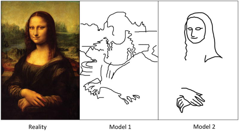
For an illustration, Leonardo’s Mona Lisa plays the role of reality. Model 1 has obviously more features and may be given preference by computer algorithms (e.g. when minimizing the rms difference), but the majority of human observers (and perhaps really smart algorithms) will likely consider Model 2 as more meaningful. A theory here can be formulated as “this is a person”, which immediately defines the most relevant features (“degrees of freedom”), yielding Model 2. Making a sketch of a painting is analogous to coarse-graining: it is not just smoothing, but rather selecting the most meaningful features and disregarding the rest. The same operation is subconsciously performed by our brain when we look at a painting from afar.

For example, issue #1 is centered on the scale of coarse-graining defined by available experimental protocols. Axons are cylinders of finite diameter, which have been quantified in animal studies using very strong diffusion gradients and narrow gradient pulses (33, 78–80), and/or in the spinal cord (78, 79, 81) where these diameters are much larger than in the brain and thus more amenable to the technical limitations of current hardware. However, diffusion times exceeding 10ms, and low diffusion weightings q in clinical scanners make both the diffusion length scale and 1/q greatly exceed the bulk of axonal diameters in the brain (~1μm), effectively coarse-graining these diameters to zero (unobservable). At such coarse-graining scales, the effective theory becomes that of “sticks” (zero-radius channels) (35, 36). Hence, for any model predicting the outcome of any diffusion sequence involving these long temporal scales and low diffusion weightings, axonal diameter becomes an irrelevant parameter (56), irrespective of model asssumptions about the orientational distribution of axons in a voxel. (Monte Carlo simulations show that for a typical clinical scenario, a gradient strength exceeding 900 mT/m would be needed to detect the attenuation from spins inside 1μm-sized axons, against a signal-to-noise ratio (SNR) of 50; on the other hand, the extra-axonal contribution dominates at low gradients.) Therefore, issue #1 is fundamentally about the theory aspect of modeling.

In contrast, as already mentioned in the Problem Section, issue #2 regarding degeneracies in the parameter estimation for multi-compartmental models of neuronal tissue at long diffusion times, is fundamentally about the parameter estimation (fitting) aspect of modeling. Successful modeling outcome involves the solution of both theory and parameter estimation aspects; both of them can be nontrivial, and their solutions generally rely on different methods and ways of thinking.

Representation = decomposition in a basis

In our experience, the word “model” is, unfortunately, often taken to be synonymous with any “approximate mathematical description of the signal”. Here we underscore – based on the physics definition above – that such descriptions, lacking a theoretical (physical) foundation, are generally not models, and propose to call them representations³ ; one may also call them data or signal interpolations (36). Developing adequate representations is often the first step in analyzing the signal.

We are not the first who try to differentiate representations from models. Already in the pre-MRI era, statisticians concerned with selecting variables in observational studies attempted to formulate this kind of challenge. Cox and Snell (83) stated in 1974: “There is a working distinction between producing (i) a fit to the data useful for future prediction in the absence of major changes in the system and (ii) an “explanation” which will link with other studies, e.g. fundamental laboratory work, and will predict under quite different circumstances. For (i), two quite different models, involving different explanatory variables, are equally acceptable if they fit the data equally well. If a choice has to be made between them, it may be done on the basis of simplicity <…>. In (ii), however, it is usually of central importance to find which explanatory variables have important effects.” Although Cox and Snell use the word “model” in the tradition of statistics⁴, it is straightforward to identify their (i) and (ii) with representations and theory/models, respectively.

More formally, a representation could be defined as a theory-independent decomposition in a basis to store, or to compress measurements. Here we understand “decomposition” quite broadly; sometimes, just one or very few suitably selected functions are enough (a low-rank representation). In contrast to models, representations are as general as possible, and have very few assumptions. As there are infinite ways to represent a continuous function, the choice of representation is often dictated by convenience or tradition. Practically, not all representations are equivalent, because one only uses a few basis functions rather than an infinite set; from this point, sparser representations are more favorable. A less obvious but very desirable requirement, from the reproducibility standpoint, is a limited sensitivity to the acquisition protocol, cf. issue #4 above (see also below for concrete examples).

A classic dMRI signal representation, using monomials 1, q², q⁴, … as the basis set for the log of signal, is the cumulant expansion (85, 86). One can look for some other convenient basis set of functions that can capture most of the information in the signal in a few parameters, e.g. the bi- or multi-exponential decay (87, 88), or expansion in the harmonic oscillator basis (89).

At this point it becomes clear that one should have very different expectations for models and for representations. Rigorously distinguishing between the two in scientific papers would help define their scope, and prevent depreciation of the considerable effort behind building and validating adequate theories/models [“explanations (ii)” per Cox and Snell]. The distinction between models and representations is thus not merely a semantic formality, as it is needed for placing published works into a broader context, and for clarifying our thinking.

DTI is not a model; neither is DKI

Consider the following example of a well-known signal representation, the Taylor expansion of the diffusion signal S_q(t) (expansion in moments), or a much more often used expansion of its logarithm (expansion in cumulants) (85, 86) already mentioned above:

$$ln{S}_q(t)=ln{S}_0-D(t)t·q^2+C(t)t^2·q^4-\dots$$ [1]

where q = |q| is proportional to the applied diffusion-sensitizing field gradient. Equivalently, this expansion can be viewed as that in the powers of the diffusion weighting parameter b = q²t at fixed diffusion time t. This leads to diffusion tensor imaging (DTI) (25) and diffusion kurtosis imaging (DKI) (90), wherein the terms D(t) and C(t) give rise to diffusion and kurtosis tensors in the presence of tissue anisotropy, probed by the direction of the vector q.

In the literature, DTI and DKI are often categorized as models. DTI, for example, is certainly a very useful approximation to the diffusion signal in a limited b-range, and it measures a well-defined physical quantity, the diffusion tensor D_ij(t), at least in the limit of narrow gradient pulses. However, according to the above logic, DTI is not actually a model, since it does not rely on any assumptions about tissue structure. The same logic, however, classifies DTI as a model for a water phantom, where the q⁴ term and beyond vanish identically. In this particular case, it is not the anisotropy (or rather its absence), but the absence of higher-order terms in Eq. [1], that constitutes a model which can be physically formulated as the absence of any structure at the micrometer scale and above.

In the general case of structured media, DTI is a diffusion signal representation based on a fundamental property – namely, the existence of a regular Taylor expansion, Eq. [1], around q = 0. Contrary to what is still often stated in the literature, DTI is not based on the Gaussian diffusion assumption either: rather, it captures only the lowest-order, q²-term, in the cumulant expansion [1]. Any reasonable biophysical model of diffusion has a DTI representation to which it reduces in the limit of low diffusion weighting. The same applies to DKI (the next-order, q⁴-term). Therefore, one cannot validate DTI or DKI (e.g., with histology): there are virtually no assumptions there. All we can do is evaluate the empirical sensitivity of diffusion and kurtosis tensor components to a given pathology; such sensitivity can already be very useful for clinical diagnosis (22), yet it does not reveal the microstructural underpinnings of the signal.

DTI and DKI are used appropriately as representations when their estimated parameters are insensitive to the range of b-values, i.e., at sufficiently small b; exceeding this range is a pitfall contributing to acquisition/modeling variability, issue #4 from the Problem Section. For instance, the diffusion tensor should be estimated when the curvature term C · b² ≪ D · b can be neglected compared with the estimated linear one (DTI); the applicability range of DKI is, respectively, determined by ensuring that the subsequent b³ ~ q⁶ term does not notably affect the estimation of D and C, and so on. Practically, this is not an easy task given realistic SNR (68, 91, 92). Fundamentally, the range of b-values for which DTI/DKI are appropriate representations is limited from above by the convergence radius of the cumulant expansion (93). Within this range, adding subsequent cumulants improves accuracy (at the cost of precision). When used beyond this range, the terminated cumulant series [1] acts as a generic polynomial approximation, for which adding an extra higher-order term changes all other terms, causing the large variability in the polynomial coefficients.

Recognizing DTI as a representation at low diffusion weighting rationalizes its widespread clinical applicability in the face of unfair criticism (“Diffusion in tissues is non-Gaussian, contrary to what DTI assumes, so DTI is wrong”). Taken literally as a model, one must indeed never use DTI; however, using it as a representation is fully justified within the b-range defined above. Proper terminology should guard against inappropriate use and interpretation of DTI or DKI by reminding of their lack of microstructural specificity, and of the need to ensure that the appropriate b-range is probed. Finally, it helps define which aspects of dMRI can be validated, and which cannot.

Stretched exponentials and anomalous diffusion

To further illustrate the dangers of using ad hoc representations, consider the stretched exponential formalism, S = S₀ exp(–(bD_S)^α). This representation is very flexible; a three-parameter fit mimics the diffusion signal in rats very well (50). However, the anomalous exponent α < 1 implies that the diffusion coefficient D ≡ –(d lnS/db)_{b → 0} defined in terms of the above expansion [1] is formally infinite, as is the mean-squared molecular displacement 〈r²〉 at any time t. This is clearly unphysical; practically, it is incompatible with DTI, and hence its fits to data will depend on the acquisition details rather than on tissue properties (cf. issue #4). It is then not surprising that the recently observed (94, 95) S ~ b^−1/2 ~ q⁻¹ scaling at large q (cf. Fig. 5C further discussed in Section Practice below), notably different from a stretched-exponential form, and originating from the Gaussian diffusion within the one-dimensional randomly-oriented neurites, explicitly invalidates this scenario in human white matter.

Figure 5. Examples of nontrivial functional dependences suitable for model validation.

(A) Deviation of diffusion coefficient in sand grains (115, 116) from its bulk value at short times is proportional to $\sqrt{t}$ (data falling onto a straight line for small $\sqrt{t}$); such a scaling is a signature of the hard-walled restrictions (14). (B) Deviation of transverse relaxation from the monoexponential form with rate constant $R_2^{\ast }$ is characterized by the derivative $\mathrm{d}{R}_2^{\ast }/\mathrm{d}t~t^{-v}$ at large t. The exponent v depends on the large-scale structural organization of tissue (122), with v = 3/2 for randomly placed impermeable spheres, and v = 2 for the so-called “maximally random jammed state” (174), in which no sphere can be moved independently from the others. Color lines show results of Monte Carlo simulations, solid black lines show corresponding analytical results and the dotted lines serve as eye guides for the predicted slope. (C) Water dMRI signal, averaged over diffusion directions, from white matter of four human subjects (colors) behaves as b^−1/2 for large b (data from ref. (94)). This can be appreciated by the data falling on a straight line when plotted as a function of b^−1/2. Black circles show the diffusion direction-averaged NAA signal from rat brain (data from ref. (35)), adjusted for the lower NAA diffusion coefficient and scaled by the T2-weighted intra-axonal water fraction to match the human data, see ref. (94). The difference between the water and NAA curves at low b are due to the extra-axonal space (EAS) contribution; the matching b^−1/2 behavior at large b illustrates qualitative similarity of water and NAA diffusion within practically impermeable “sticks” (zero-radius cylinders), while the EAS contribution becomes exponentially suppressed. (D) The signal in the Callaghan’s model changes radically, becoming monoxeponential, when measured with the isotropic diffusion weighting (125–127).

A related phenomenon with less dramatic consequences, sometimes invoked for tissues, is the so-called anomalous diffusion (53, 96, 97), cf. issue #3 above, where the second moment 〈r²〉 may exist, but grows asymptotically with time as 〈r²〉 ~ t^v, v ≠ 1, as t → ∞. (Normal diffusion corresponds to v = 1 asymptotically (53).) Fits again look great in the finite time range in the brain (51); however, taken literally, the macroscopic diffusion coefficient D_∞ ∝ [〈r²〉/t]_{t → ∞} is either zero (when v < 1) or infinite (when v < 1). Neither value is supported experimentally; the overwhelming experience is that the time-dependent diffusion coefficient D(t) approaches a finite value D_∞ > 0 as t → ∞ (55, 67, 98, 99). Practically, this again means that the fit results are determined by the employed range (in this case, of t), rather than by the tissue itself, contributing to the issue #4 of acqusition/modeling variability.

Fundamentally, anomalous diffusion can emerge as a result of a very broad distribution of elementary time-steps or hopping distances for random walkers (53), pointing at some kind of anomalous heterogeneity of system’s properties. This is a very stringent and exotic condition; it is no wonder that the overwhelming majority of systems do not fulfill this requirement and instead fall in the wide basin of attraction of the central limit theorem (for which v = 1 (53). Importantly, the heterogeneity required for v ≠ 1 has not been observed in tissues, at least at the diffusion length scales that we usually study – for example, a recent investigation (54) using histology of white matter tracts points at a finite correlation length, consistent with a finite tortuosity limit D_∞ and asymptotically “normal” diffusion characterized by exponent v = 1

Both the stretched-exponential and anomalous-diffusion examples illustrate the above statement that a representation does not have predictive power outside the data range used for the fitting, and serve as a precaution for using representations whose basis functions are incompatible with the physical origins of the signal.

Representations are sensitive; models strive to be specific

By design, a theory, and models derived on its basis, have limited scope of applicability; their main advantage is specificity. A theory tells us which biophysical parameters – e.g. cell water fraction, membrane permeability – are relevant, i.e., are absolutely necessary to predict the measurement, and, consequently, can be quantified given sufficient data quality. Attaining specificity rather than just sensitivity is much harder, but has much more potential impact. We believe it is one of the most promising goals of microstructural mapping.

Are all models wrong? (Box vs. Cox)

George Box famously said (100) “All models are wrong but some are useful”. As this quote is becoming popular in discussions within our scientific community, we are concerned that it will be misused as a justification for a certain intellectual relativism (if all models are wrong, why try so hard?). Fortunately, not all statisticians agree with Box. Notably, David Cox says in his comment on ref. (101): “Finally it does not seem helpful just to say that all models are wrong. The very word model implies simplification and idealization. The idea that complex physical, biological or sociological systems can be exactly described by a few formulae is patently absurd.” We agree with Cox, as he clearly means “model” as derived from a theory. The key word here is “simplification” – theories are approximations by design, and the achieved simplification (per modern physics viewpoint, due to coarse-graining over the shorter-scale degrees of freedom) is their key strength.

Representations can be viewed as an intermediate step, to store a measurement for future use, before an adequate theory is settled on; for empirical correlation of the basis coefficients with pathology; and for model parameter estimation, by comparing, e.g., corresponding Taylor coefficients of the signal and of the model (38, 43, 102). Representations can be extremely useful, as they can parsimoniously capture the behavior of the signal and can provide clinically valuable markers with high sensitivity. However, in the grand scheme of things, they are the means rather than the goal.

Box’s quote may become acceptable in the following form: All representations are wrong, but some are useful. On the other hand, if we talk about genuine models, then, for a given spatio-temporal scale (reflecting the level of coarse-graining), there is only one correct theory, and all the others are, consequently, incorrect. The correct theory is very, very useful. Validating such theory is very, very hard. We end up returning to the same assumptions multiple times, trying to see where they break down. Perhaps this is why it’s called research rather than search.

A model detached from its roots becomes a representation

Modeling and representing are not mutually exclusive ways to proceed; frequently, one researcher is involved in both. Moreover, the borderline between models and representations can be subtle, and it is increasingly important to realize on which side we are in any given situation or problem. A model detached from its theoretical origin, i.e., from a specific picture of microstructure or system composition, becomes a representation.

For example, the biexponential model of diffusion is an appropriate model of two Gaussian compartments without exchange. However, it is a representation outside this original context. Its enormous mathematical flexibility as a representation, for better or for worse, is illustrated in Figure 3. One can claim a biexponential to be a genuine model only if one really has reasons to assume two compartments with Gaussian diffusion (or monoexponential relaxation); justifying this assumption is much less trivial and much more impactful than performing biexponential fitting. To generalize, performing a multiexponential fit (equivalent to the Laplace transform) without identifying meaningful non-exchanging Gaussian compartments is not modeling either – it’s just a change of basis.

Figure 3. The mathematical flexibility of the biexponential representation.

Fitting a biexponential function S = f₁e^−bD₁ + f₂e^−bD₂, with f₁ + f₂ = 1, to the noise-free Callaghan’s model (6) of diffusion inside isotropically distributed one-dimensional channels, with the exact signal expression (16, 35) shown in panel A. D_|| is the diffusivity along the channels. The substantial mathematical difference in signal expressions does not prevent the biexponential function to achieve a very high fit quality (A). The inadequacy of the biexponential representation becomes apparent only for extremely large bD_|| (B), or from the dependence of its fit parameters on the range of data used for fitting (C). In these simulations, 1001 b-values were uniformly distributed from 0 to b_max.

In a similar vein, fixing certain model parameters (or introducing stringent priors), strictly speaking transforms a physical model into a representation, unless there are compelling reasons to believe we really know these parameter values, and that they do not change in the pathology we are studying. For instance, in the brain diffusion community there is an ongoing debate (42, 43, 48) on how well we know the values of compartment diffusivities and what is the effect of fixing their values (32, 39, 44) in the Standard Model (46), cf. issue #2 in the Problem Section. Expressions involving un-validated constraints merely interpolate the dMRI measurement; the bar for providing its microstructural explanation and for revealing biophysical parameter trends in disease is much higher.

Practice

Fit quality does not validate a model

While Figure 3 demonstrates the fascinating flexibility of the biexponential representation, Figure 4 shows how well other fundamentally distinct mathematical functions (representations) can fit the same data, with the ground truth in this example being biexponential. A hint about the reason for such ambiguity comes from the cumulant expansion [1], which renders all diffusion-weighted signals accurately represented by diffusion and kurtosis terms for the low diffusion weightings typically used in clinical settings (93).

Figure 4. Quality of fit alone does not validate a model: the wrong expression sometimes fits better than the true model.

A biexponential signal S = 0.8e^−1.2b + 0.2e^−0.2b was computed for b-values from 0 to 3.5 in steps of 0.5 (all below the convergence radius (93) of the cumulant expansion (85)). Fitting quality of the three representations was compared over 10,000 realizations of additive Gaussian noise: the cumulant expansion S = S₀ e^−bD+kb2 (terminated at the kurtosis term), the biexponential, and the stretched exponential function, with the number of adjustable parameters 3, 4 and 3, respectively. The initial values for the fitting of the biexponential and stretched exponential functions were generated using the ground truth. The distributions of the corresponding corrected Akaike information criterion (AICc) (172, 173) is shown for the increasing noise level (panels A to C). AICc represents χ² penalized by the number of fit degrees of freedom; the smaller AICc, the better the fit quality. (A) AICc values prefer the ground truth (bi-exp) for extremely low noise. (B) Increase in the noise to more realistic levels makes the cumulant expansion perform better due to the fewer number of parameters. (C) For the clinically realistic SNR = 20, AICc for the correct model is the worst. In this case, the intrinsic inaccuracy of the representations is completely masked by the noise, therefore AICc is dominated by the penalty term for the number of degrees of freedom. Vertical solid lines in all panels show the mean of distributions, while vertical dashed lines show the corresponding theoretical estimates.

These examples emphasize that fitting quality (embodied, e.g. by R², or by Akaike Information Criterion) is not necessarily a signature of the correct model — and may even prefer wrong models over the right one (Fig. 4C). Good fitting quality of a derived model is a necessary, but not a sufficient condition for validity of the underlying theory. In dMRI, for instance, many expressions fit data extremely well in the clinical range of t and q, yet very few of them are proven to be correct models.

To further quote D. R. Cox (in his discussion of ref. (101)): “Within a given broad framework it may be essential to recognize explicitly that different models with different interpretations fit about equally well; procedures which then force a single choice are bound to be potentially misleading.” We believe that this wisdom applies whether the choice is between a few models (Figure 4) or dozens of them (103, 104).

Validate theories and derived models, not representations

In general, representations cannot be validated by their very definition. They can be judged by their fitting quality, parsimony, applicability range, flexibility and sensitivity – and maybe even elegance.

Theories and the derived models, however, must be validated, and currently this may be our greatest challenge. Although a highly valuable means of validation, even histology often cannot provide the gold standard for in vivo MRI: besides suffering from hard-to-control changes in tissue properties caused by sample preparation (105), it is in principle insensitive to MRI-specific parameters such as diffusivities and relaxation rates in different tissue compartments. How do we overcome this validation challenge?

Validate models where they exhibit distinctive functional dependencies

This problem is not new. Physicists have struggled with it all the time: How can we “see”, e.g., the internal structure of a proton? There is no histology there; our only way is to bombard a proton with other particles – say, electrons, – and to study the indirect effect of the constituent parts (the quarks, as it turned out) via deep inelastic scattering. The key is to have a detailed theory (at a given coarse-graining length scale) of how the result of such an experiment depends on the kinetic energy of electrons and on the proton structure. By identifying the expected features in such functional dependencies, remarkably far-reaching conclusions about the structure of elementary particles have been made (106, 107). We underscore that all such understanding has been achieved indirectly without any alternative validation – solely based on the observed functional forms.

In other words, it is pointless to perform model selection in a regime where they all look similar. We should instead drive the measurements into domains where different physical assumptions lead to qualitatively distinct functional forms of theoretical predictions. By validating the model where it is distinctive, we amplify the role of its physical assumptions and learn something definitive.

This tradition has yet to fully percolate into our burgeoning field. This is especially necessary in view of the featurelessness of, e.g., commonly acquired dMRI signal as a function of b, which is famously regarded as “uninformative” or “remarkably unremarkable” (108, 109). The reason for such an unfortunate property in dMRI is again the validity of the cumulant expansion, Eq. [1] above: all models predict similar-looking signals for low b-values (68).

A few fortunate examples of breaking through the fog of a featureless MR signal include:

• Identifying the diffusion narrowing regime in the mesoscopic transverse relaxation via the $B_0^2$ scaling of the $R_2^{\ast }$ rate, helping to validate models which enable quantification of iron in the brain (75) and contrast agent in blood (110).

• A scaling law (111–113) derived from the Bloch-Torrey equation helped to simplify the parametric dependence of transverse relaxation rate caused by blood pool contrast agents, and to explain the increased sensitivity to the microvasculature for increasing contrast concentration (114).

• Observation of the $\sqrt{t}$ decrease of D(t) at short diffusion times (14) in porous media (115, 116) (Fig. 5A), in a fiber phantom (117), in cell suspensions (118), and in vivo in breast (119) and in brain tumors (120).

• Effect of structural disorder on the time-dependent diffusion, relating structural fluctuations of a heterogeneous media to the diffusive dynamics. Technically, this is embodied by the relation (67) between the power-law exponent p in the low-k scaling of the power spectrum Γ(k) ~ k^p of restrictions to diffusion, and the dynamical power-law exponent υ describing the approach of time-dependent diffusion coefficient to its long-time (tortuosity) limit D_∞. This relation was validated in phantoms (54, 121), and it practically helps in the model selection. For instance, it was used to argue that axons are not just straight hollow tubes from the diffusion standpoint, and are characterized by short-range disorder along them (55). The diffusion time-dependence in cortical gray matter (99), and the diffusion coefficient drop in stroke, were explained in tems of of this structural one-dimensional disorder along the neurites in the brain, and its increase in ischemia (67).

• Effect of structural disorder on the time-dependent transverse relaxation (Fig. 5B), relating structural fluctuations of a heterogeneous magnetic media to the relaxational dynamics. Technically, this is embodied by the relation between the power-law exponent in the low-k scaling of the power spectrum Γ_χ(k) of heterogeneous magnetic susceptibility, and the dynamical power-law exponent describing the approach of time-dependent transverse relaxation rate $R_2^{\ast }(t)$ to its constant value $R_2^{\ast }(\infty )$ for long times (71, 75, 122).

• Effects of laminar flow and multiple generations of vasculature on the functional form of the impulse response function that describes blood pool tracer propagation in the brain vasculature (123).

As a further illustration, Fig. 5C shows how one can potentially validate the picture of neurites as infinitely narrow “sticks”, by studying the nontrivial power-law form S ~ b^−1/2 of the diffusion signal at large b (94, 95). The functional form S ~ b^−1/2 ~ q⁻¹ at large b (and fixed t) restricts the family of dMRI models in human brain white matter so strongly, that it (i) excludes observable effects of inner axonal diameters on regular human scanners (cf. Issue #1); (ii) invalidates, to the best of our understanding, the picture of water bound to membranes (124) (as that would yield notable positive intercept S|_{b → ∞} given by the stationary water fraction); and (iii) reveals that the so-called (differential) return-to-origin probability $\text{RTOP}=\int \frac{d^{3}q}{{(2\pi )}^3}S(t,q)~\int \frac{d^{3}q}{q}=\infty$ would diverge in brain white matter if S ~ 1/q for q → ∞. The spurious RTOP divergence gets cut-off at much higher q, of the order of inverse axonal diameter, beyond which S should decrease exponentially. Consider then RTOP maps (89), calculated from brain dMRI signal acquired in the b-range where the deviations from the scaling ~ b^−1/2 are unobservable. The above divergence will make such maps mostly depend on the largest b-shell of the acquisition (providing an artificial cut-off for the above diverging integral), rather than on the tissue properties, cf. reproducibiity issue #4.

The last RTOP example also illustrates that not all representations are created equal. The harmonic oscillator basis (89) is good for representing signals that are close to a Gaussian. However, not including the slowly decaying function ~1/q, this representation requires a lot of exponentially decaying and oscillating terms to converge for fitting the actual signal. Hence, it is practically suboptimal for the central nervous system. This unexpected pitfall illustrates our broader point: Applied challenges are often fundamental problems in disguise. Even such a practical problem as interpreting the expansion coefficients of a dMRI signal in a seemingly innocuous basis can have pitfalls stemming from the nontrivial fundamental origins of the signal.

Further validation: Alter functional dependencies by applying “orthogonal” measurement schemes

A defining property of a theory is its ability to predict the outcome of a different measurement on the same system (at the same level of coarse-graining). Figure 5D illustrates this point on the earlier example of Callaghan’s model introduced in Figure 3. In this case, isotropic diffusion weighting, which results in signal suppression if water can move in any spatial direction, and thus cannot be replicated by the conventional (single-direction) diffusion encoding measurement schemes, yields an essentially different – monoexponential – functional form (125–127). This principle has recently been applied in a more complex situation of water diffusion in the human brain (49, 128). We believe that multiple diffusion encoding schemes (128–133), which have been gaining popularity recently, can provide distinct functional forms of the models suitable for validation.

Complementary MRI modalities offer promising synergies for microstructure parameter estimation: e.g., myelin water fraction, estimated via T₂ mapping or magnetization transfer (134–138), may subsequently be fed into diffusion modelling; varying the echo time (139) helps cure the inherent degeneracy in the free water elimination problem (140–142), which is most pronounced when used on a single-shell DTI (141); employing both the echo time dimension (143) and multiple diffusion encodings (144) helps to lift the degeneracy in white matter parameter estimation, cf. issue #2 from the Problem Section.

We underscore that all these diverse “orthogonal” methods are beneficial not just for robust parameter estimation, but also for the more fundamental goal of theory validation, by providing different facets of the same physical reality and testing an overall consistency of our physical assumptions. Representations do not have such a predictive power.

Information content and new contrasts: Where is value?

While sparse representations can give us a good idea about how many basis functions are needed to reproduce the signal, theory defines the ultimate information content, since it identifies the biophysically relevant parameters. It tells what is in principle possible to measure, and what is not. Any claim of a “novel contrast” should be scrutinized: does the technique reveal the previously unattainable degrees of freedom, or can its results be re-generated using conventional measurements?

Considering specific examples, the value of the cumulant representation [1] at low diffusion weighting is manifest in restricting the functional form –ln(S_q/S₀) = Σ_ij D_ijq_iq_jt + ··· to the second-rank tensor D_ij, equivalent to expanding the signal in spherical harmonics (SH) up to l = 2; likewise, if the signal is well approximated by the terms up to b², DKI sets maximal SH order l = 4, and so on (85, 145). This general radial-angular connection in the q-space (43) implies that, for HARDI data at b ~ 1000 ms/mm², where DTI (and at most DKI) are enough to represent the signal, employing SH with orders above l = 4 is counterproductive, as it leads to overfitting. Here, the sparsity of representation [1] is twofold: involving terms ~q^l with only even orders l is set by the time-translation invariance of the Brownian motion, while the limit on the number of independent tensor components in each cumulant term is set by counting the dimensions of irreducible representations of the SO(3) rotation group (43).

Theory allows us to go one step further in limiting the number of parameters. In the above example (54) of the extra-axonal diffusivity D(t) ≃ D_∞ + A (ln t)/t transverse to fiber tracts approaching its t = ∞ limit D_∞, the corresponding kurtosis K ≃ (6A/D_∞) (ln t)/t approaches zero in a way completely defined by the effective medium parameters D_∞ and A. Therefore, in this limit, kurtosis in the extra-axonal space does not provide independent contrast, even though it is viewed as an independent parameter in the cumulant series representation [1]. Here, theory can add value in constraining the functional form of the signal, thereby minimizing the number of independent parameters to be estimated and, hence, maximizing their precision.

Sometimes, unconventional acquisitions can create an appearance of providing new contrast. Multiple diffusion encodings (130, 131), such as double PFG, appear quite different from the conventional pulsed-field gradient (PFG) sequence. However, they provide novel contrast only starting from the O(q⁴) level (146), while at the O(q²) level the result of any diffusion encoding can be fully synthesized from the knowledge of the time-dependent diffusion tensor (147, 148) that can be measured with conventional DTI by varying the diffusion time t. In this case, theory helps understand how far one needs to push an acquisition to become truly valuable.

Conversely, empirically informative acquisitions may mask problems with modeling. A multi-shell dMRI acquisition, involving up to, say, b ~ 2,000 – 3,000 s/mm² and a multitude of directions, is empirically much more informative than DTI at b ~ 500 s/mm². Almost any plausible metric, physically sound or not, derived from such a rich acquisition, may turn out to be more sensitive to pathology than the diffusion tensor. This should not be viewed as an automatic justification of such metrics to be more “valuable” than, say, DTI. If the theory is wrong or the fitting is biased, the added value does not lie in the modeling, but rather in the high-b acquisition, and the whole pipeline becomes more informative not because the modeling is so great, but if anything, in spite of it. If unsure about a modeling framework, it may be more intellectually honest (and valuable) to stay at the level of a representation, foregoing microstructural specificity; for instance, in the above example, a metric such as mean kurtosis (149) will be sensitive to many pathological and developmental changes (150–154). Of course, ultimately, we would like to become specific, not just sensitive. However, a wrong theory or a biased estimation does not help achieve specificity, which is why the choice between modeling and representing is nontrivial, akin to striking the right balance between what we can claim and what we cannot.

Discussion

Uncover a little rather than cover a lot

Each careful validation study — e.g. a proven constraint on the model’s functional form, and hence, on the relevant microstructural degrees of freedom — may seem to be a small and incredibly tedious step for a researcher, but it is a giant step for the scientific community. This is because its ripples are exponentially propelled into the future, eliminating a snowballing array of choices for a model candidate in all future studies. From that point onward, all models for a given tissue (at that coarse-graining scale) should obey this constraint! Cumulatively, this saves all of us enormous amount of time and resources.

Blind and premature push-button fitting, conversely, gives us a false sense of achievement. It is relatively easy to produce a lot of output. Unfortunately, this is merely a way to produce more incorrect results faster, which would inevitably prompt the need for a fairly depressing effort to re-assess all of them at some future point. Since, as we pointed out above, an unphysical parametric map does not immediately create discomfort, it pays to make a very conscious effort to get alarmed and question our own results earlier rather than later.

We note that model validation, involving driving acquisition to the limit of hardware and acquisition time for identifying a nontrivial functional form, is usually incompatible with routine clinical protocols. This represents a distinction between the basic and applied research: pushing the boundaries is meant to be difficult and rare, whereas the point of developing applications is to make them user-friendly. Once the correct theory/model is established, there is no need to validate it in every patient – instead, one can begin optimizing both acquisition and parameter estimation, to reach acceptable precision for the parameters relevant to a particular clinical situation and suspected pathology.

Which model is right?

“I am a clinician, I am lost – how do I know I am using the right model for my study?” A short answer is, you don’t – much like we have no idea how to recognize a sound radiology report. Achieving sufficient qualification either in modeling or in the clinical work requires many years of highly specialized training.

One question that can be answered relatively easily is whether it is really a model, or a representation; this realization could already help placing results of the study into a proper scientific context. For that, the following empirical rule is helpful: Models are pictures, while representations are formulas (46). Describing genuine models always entails creating a sketch of the relevant parts of microstructure, while representations are just some sets of functions.

An ultimate answer to the above question lies in creating an active modeling community in the area of microstructual mapping (spanning diffusion, transverse relaxation, magnetization transfer, quantitative susceptibility mapping, and perfusion, at the very least), that fulfills the two functions: (i) building new theories and models, and (ii) maintaining our common knowledge base by constantly questioning existing models and subjecting them to novel validation methods. Then virtually anyone from such community could give a widely-accepted answer to this question. In the absence of a common theoretical ground, the answer too often depends on whom you ask.

One of the major lessons learned from the progress fundamental physics has achieved over the past century, is how much theory has played a role in it. Building the modeling community involves an investment: specialized training for junior scientists; enabling a career path in modeling; conducting targeted workshops; and stimulating theory-focused publications. This investment pays off by informing the discussion of new acquisition methods, designing novel contrasts and biomarkers based on objective tissue characteristics, as well as by saving us enormous resources and time in not pursuing costly studies based on unsound quantitative methods.

To model or to represent?

If modeling is hard, and validation is even harder, why bother? As argued above, building and validating an adequate theory achieves an overarching scientific milestone, by identifying relevant tissue properties that manifest themselves in the voxel-wise MRI signal. This fundamental milestone, reflected in our ability to predict the response of the tissue to other independent measurements, unveils the information content of our acquisitions, and opens up the following practical avenues:

1. Modeling offers unforeseen insights into optimizing or discovering novel acquisitions and independent contrasts, feeding the next generation of technical MRI development;

2. Unbiased estimation of relevant tissue parameters is key to the ultimate harmonization of measurements across vendors and sites, with a potential to achieve maximal possible statistical power and reproducibility in large-scale studies, limited only by the inherent biological variability;

3. Building microstructural maps could connect our field in a whole new way to the basic biology and neuroscience, translating our fundamental insights into a new kind of multi-modal super-resolution microscopy.

Clinically though, one could argue that staying at the level of parsimonious representations could be sufficient – if we can robustly correlate empirical basis coefficients with pathology. The classic example of the diffusion coefficient drop in stroke (22) can be viewed as a case supporting this viewpoint. At the very least, limiting ourselves to representations allows us to stay intellectually honest yet already clinically useful in some cases.

It seems that the choice between modeling and representing depends on how ambitious we want to be. In a sufficiently complex pathology – e.g. Alzheimer’s disease or multiple sclerosis – the earliest-stage pathological processes should change the signal only in very subtle ways. Early detection effectively means amplifying these changes by some analysis scheme. This, formally, can be regarded as applying a certain nonlinear transformation to the measured data, as well as performing the measurement within the most optimal domain in the parameter space. One can intuitively expect that the more complex the measurement and the pathology, the wider the search space is for finding the most optimal data transformation and measurement paradigm, and the less chances a simple guess, or a basis coefficient, would have. We can view biophysical modeling as a constructive path to uncover such a transformation together with suggesting optimal measurement parameters or even new measurement paradigms. While one can sometimes arrive at them by serendipity, or, possibly, by mining enormous data sets acquired using the broadest possible range of sequence settings and MR modalities, the history of science tells us that building our insight through a combination of theory and experiment is the most powerful and certain way of reaching this goal.

Fundamental or applied?

As a premise of our article, we posited that progress in microstructural mapping may hinge on our ability to recognize fundamental problems behind building applications. Making such distinction is easy, perhaps, only in retrospect. Here, our community is not an exception – the fundamental nature of the seemingly applied challenges has often been missed in other fields.

One may recall the “reductionist” trend (155) in the glory days of high-energy physics, to selectively classify only the elementary-particles and nuclear physics as “intensive” science, painting all other fields as “extensive”, with no fundamental problems to overcome, which often associated condensed matter physics with device engineering. Countering this trend, in the inspirational article “More is Different” (61) Philip Anderson formulated the hierarchical nature of science: “At each level of complexity entirely new properties appear, and the understanding of the new behaviors requires research which I think is as fundamental in its nature as any other.” Truly remarkable developments in condensed matter physics over the past half-century have proven this point decisively: Complexity both due to interactions between many particles, and due to effects of a disordered environment, has been understood to result in fundamentally new effective theories of emergent collective behavior. Besides, engineering the new generation of devices employing quantum information requires fundamental advances (156, 157).

Similarly, at the dawn of quantum theory a century ago, Planck’s formula for the spectral shape of the black-body radiation was first written down merely as a representation of experimental data (158, 159), where the quantum of energy was introduced as a computational trick to calculate the entropy of a continuous energy distribution. Meanwhile, Ritz attempted to explain the atomic spectra in the spirit of classical mechanics as eigenfrequencies of elementary elastic membranes (160, 161). We know today how far these efforts were from reality. In both cases, truly revolutionary progress only came when the fundamental physical assumptions behind the empirical formulas were fully appreciated.

Recognizing the fundamental problems early on will help us to adjust our strategy: Avoid premature optimization (in the words of Donald Knuth, “the root of all evil” (162)), and rather spend most of our efforts on understanding and validating. As we noted in the Theory section, in every kind of measurement, there exists only one correct theory/model, as opposed to many equivalent ways to represent a signal. This is why basic scientists spend so much time arguing about model assumptions. “To describe a signal”, any basis would do; to understand nature, only one model has meaning, even though its goodness-of-fit may not necessarily be superior to other representations in a routine measurement.

What are the other fundamental challenges in our ever-changing field that are mischaracterized as merely applied hurdles? Do the modern neural-network-based approaches to image classification (163) and reconstruction (164) contain enough complexity, that “learning” itself can be regarded as a fundamentally new, emergent phenomenon (165)? Can one rigorously formulate the optimal ratio of time spent on (under)sampling the k-space (to localize images) vs. probing the microstructural information (e.g., by sampling the echo time, the q-space, etc) – aren’t we spending too much time localizing while not spending enough on probing microstructure?

Micro + macro: In search of convergence

The distinction between models and representations prompts looking from a different angle at the stimulating ideas of compressed sensing (166) and MR fingerprinting (167). From the present point, compressed sensing involves a search for the sparsest possible basis for representing the signal. In contrast, MR fingerprinting (MRF) is parameter estimation of a theory (e.g. expressed by the Bloch equation); this theory is used to generate a model (a library of fingerprints), with model fitting implemented in terms of an exhaustive library search.

For compressed sensing, while ad hoc sparce image representations have been useful, the best signal compression should be achieved when one uses the genuine biophysical model – the one containing only the relevant degrees of freedom (i.e., by definition, the minimal number of parameters, together with correct functional form for a given measurement technique). In other words, the genuine biophysical model is going to be sparser than any representation.

For the MRF, having an adequate theory is arguably even more crucial, as it serves as a foundation for the library-based parameter estimation. Both macroscopic effects due to hardware imperfections (168), and microstructural effects (169) making spin dynamics deviate from that based on simple Bloch equations, should affect the library and the estimated parameters. While we limited our discussion to dMRI (typically not part of MRF protocols), we belive that the overarching issues of rigorous modeling and validation are essential for the MRF development, e.g. when including effects of magnetization transfer and of the mesoscopic $R_2^{\ast }$ relaxation. A potentially exciting yet untested synergy could lie in novel acquisition/estimation paradigms, such as MRF, helping validate theories by providing densest possible data sampling. On the other hand, inadequate models used as basis for MRF libraries carry the danger of creating biased parameter maps in multiple modalities.

Overall, deriving and validating adequate theories is crucial for both compressed sensing and MRF. This realization adds a modern meaning to the timeless wisdom of Ludwig Boltzmann: There is nothing more practical than a good theory. This point of convergence between the microstructural modeling and the (macroscopic) image reconstruction puts an even stronger emphasis on developing and validating biophysical models, and on forming an interdisciplinary theory community focussed on quantifying tissue microstructure from multiple angles. We hope this potential synergy could bring together researchers from microstructure and image reconstruction, and would result in employing the sparsest possible functional forms to achieve a qualitatively faster and more precise reconstruction of biophysical parametric maps directly, perhaps eventually bypassing the “weighted” images all together.

A universal language

Striving for the intellectual rigor – a prerequisite for developing adequate mathematical descriptions of natural phenomena – has benefited virtually every scientific field. The ability to define assumptions and build theories reflects an overall degree of progress in a given area, as well as helps connect it to the previously developed body of science. These connections can be incredibly powerful and enriching: when speaking the same mathematical language, seemingly distinct scientific disciplines can exchange knowledge. Eugene Wigner formulated this observation in terms of “the unreasonable effectiveness of mathematics in natural sciences” (170), referring to the appropriateness of mathematical formulation of the laws of nature as the empirical law of epistemology. He underscored that, while mathematical concepts are chosen not for their simplicity (often they are far from simple), they are rather employed “for their amenability to clever manipulations and to striking, brilliant arguments”. Biology still needs such a language, as it was insightfully and hilariously illustrated by addressing the question “Can a biologist fix a radio” (171). Poised between physics and biology, our MRI community may be in a unique position to convey a well-established rigorous language of the physical sciences into the life sciences.

Having made tremendous progress in building the engineering marvels that are the modern-day MRI scanners, and in creating exquisite image processing and reconstruction tools, we are still trying to do what John Tanner had been doing already in the 1970s when quantifying microstructure of a frog muscle (5): modeling tissue as a simplified microgeometry, performing an NMR measurement, and estimating the model parameters. On second thought, it is not surprising – nothing fundamentally has changed in the way science is done: theory, parameter estimation from the measurement, and model validation were as fundamental to the scientific enterprise in the 1970s as they are now. Developing adequate models with the far more advanced measurement tools of today brings us back to our scientific roots.

Theory development and validation will connect us with the physical and the life sciences. Even if details of our hardware and acquisition may remain obscure to outsiders, our results, whenever sufficiently rigorous and expressed in the commonly accepted scientific terms, are bound to evoke interest from other branches of science. Borrowing methodology from physics, and quantitative measurements of tissue parameters from biology, will not just help us design methods that could turn our aspirations into clinical reality, but will also provide a universal language to share our successes with other fields, and will help our community occupy its rightful place at the crossroads of physics, chemistry, biology and neuroscience.

Summary.

To unleash the full potential of model-based microstructural mapping, we formulated and answered the two fundamental questions. The theoretical question (What is a model?) involves drawing a distinction between a theory, involving relevant microstructural degrees of freedom, and a representation, which is a mere decomposition of a measurement in a convenient basis. The experimental question (How to validate?) can be addressed by (i) uncovering functional forms of models specific to their defining physical assumptions, and (ii) predicting and comparing with the outcomes of “orthogonal” measurements that involve fundamentally the same physical degrees of freedom, but provide independent combinations of relevant parameters of the theory.

We believe that approaching microstructural challenges with an increased rigor and a logic of a basic science is not a luxury at this point, but a method of investigation necessary to reach tangible practical advances. We should strive to identify relevant degrees of freedom when interpreting any MRI measurement – in other words, listen to what nature offers, rather than insist on what we wish to have. This can be accomplished by changing the culture towards recognizing that microstructural mapping requires solving fundamental problems. This entails investing in basic research, i.e., in the modeling and validation studies, as key to future applications; focussing on calibration and reproducibility; educating a new generation of scholars in modern theory and validation methods; and actively building bridges with the broader scientific community beyond our regular ISMRM meetings and workshops, using theory and validation studies as a universal language transcending different fields. Other disciplines need us, and we need them.

References

- 1.Abbe E. Beiträge zur Theorie des Mikroskops und der mikroskopischen Wahrnehmung. Archiv für mikroskopische Anatomie. 1873;9(1):413–8. [Google Scholar]
- 2.Betzig E. Nobel Lecture: Single molecules, cells, and super-resolution optics. Rev Mod Phys. 2015;87(4) doi: 10.1103/RevModPhys.87.1153. [DOI] [PubMed] [Google Scholar]
- 3.Hell SW. Nobel Lecture: Nanoscopy with freely propagating light. Rev Mod Phys. 2015;87(4) doi: 10.1103/RevModPhys.87.1169. [DOI] [Google Scholar]
- 4.Moerner WE. Nobel Lecture: Single-molecule spectroscopy, imaging, and photocontrol: Foundations for super-resolution microscopy. Rev Mod Phys. 2015;87(4) doi: 10.1103/RevModPhys.87.1183. [DOI] [PubMed] [Google Scholar]
- 5.Tanner JE. Self diffusion of water in frog muscle. Biophys J. 1979;28(1):107–16. doi: 10.1016/S0006-3495(79)85162-0. [DOI] [PMC free article] [PubMed] [Google Scholar]
- 6.Callaghan PT, Jolley KW, Lelievre J. Diffusion of water in the endosperm tissue of wheat grains as studied by pulsed field gradient nuclear magnetic resonance. Biophys J. 1979;28(1):133–41. doi: 10.1016/S0006-3495(79)85164-4. [DOI] [PMC free article] [PubMed] [Google Scholar]
- 7.Yablonskiy DA, Haacke EM. Theory of NMR signal behavior in magnetically inhomogeneous tissues: the static dephasing regime. Magn Reson Med. 1994;32(6):749–63. doi: 10.1002/mrm.1910320610. [DOI] [PubMed] [Google Scholar]
- 8.Boxerman JL, Bandettini PA, Kwong KK, Baker JR, Davis TL, Rosen BR, Weisskoff RM. The intravascular contribution to fMRI signal change: Monte Carlo modeling and diffusion-weighted studies in vivo. Magn Reson Med. 1995;34(1):4–10. doi: 10.1002/mrm.1910340103. [DOI] [PubMed] [Google Scholar]
- 9.Le Bihan D, Breton E, Lallemand D, Grenier P, Cabanis E, Laval-Jeantet M. MR imaging of intravoxel incoherent motions: application to diffusion and perfusion in neurologic disorders. Radiology. 1986;161(2):401–7. doi: 10.1148/radiology.161.2.3763909. [DOI] [PubMed] [Google Scholar]
- 10.Callaghan PT, Eccles CD, Xia Y. NMR microscopy of dynamic displacements: k-space and q-space imaging. J Phys E: Sci Instrum. 1988;21:820–2. [Google Scholar]
- 11.Stanisz GJ, Szafer A, Wright GA, Henkelman RM. An analytical model of restricted diffusion in bovine optic nerve. Magn Reson Med. 1997;37(1):103–11. doi: 10.1002/mrm.1910370115. [DOI] [PubMed] [Google Scholar]
- 12.Szafer A, Zhong J, Gore JC. Theoretical model for water diffusion in tissues. Magn Reson Med. 1995;33(5):697–712. doi: 10.1002/mrm.1910330516. [DOI] [PubMed] [Google Scholar]
- 13.Cory DG, Garroway AN. Measurement of translational displacement probabilities by NMR: an indicator of compartmentation. Magn Reson Med. 1990;14(3):435–44. doi: 10.1002/mrm.1910140303. [DOI] [PubMed] [Google Scholar]
- 14.Mitra PP, Sen PN, Schwartz LM. Short-time behavior of the diffusion coefficient as a geometrical probe of porous media. Phys Rev B Condens Matter. 1993;47(14):8565–74. doi: 10.1103/physrevb.47.8565. [DOI] [PubMed] [Google Scholar]
- 15.Mitra PP, Sen PN, Schwartz LM, Le Doussal P. Diffusion propagator as a probe of the structure of porous media. Phys Rev Lett. 1992;68(24):3555–8. doi: 10.1103/PhysRevLett.68.3555. [DOI] [PubMed] [Google Scholar]
- 16.Yablonskiy DA, Sukstanskii AL, Leawoods JC, Gierada DS, Bretthorst GL, Lefrak SS, Cooper JD, Conradi MS. Quantitative in vivo assessment of lung microstructure at the alveolar level with hyperpolarized 3He diffusion MRI. Proc Natl Acad Sci U S A. 2002;99(5):3111–6. doi: 10.1073/pnas.052594699. [DOI] [PMC free article] [PubMed] [Google Scholar]
- 17.Wang J, Fernandez-Seara MA, Wang S, St Lawrence KS. When perfusion meets diffusion: in vivo measurement of water permeability in human brain. J Cereb Blood Flow Metab. 2007;27(4):839–49. doi: 10.1038/sj.jcbfm.9600398. [DOI] [PubMed] [Google Scholar]
- 18.Gregori J, Schuff N, Kern R, Gunther M. T2-based arterial spin labeling measurements of blood to tissue water transfer in human brain. J Magn Reson Imaging. 2013;37(2):332–42. doi: 10.1002/jmri.23822. [DOI] [PMC free article] [PubMed] [Google Scholar]
- 19.He X, Yablonskiy DA. Biophysical mechanisms of phase contrast in gradient echo MRI. Proc Natl Acad Sci U S A. 2009;106(32):13558–63. doi: 10.1073/pnas.0904899106. [DOI] [PMC free article] [PubMed] [Google Scholar]
- 20.Duyn JH, van Gelderen P, Li TQ, de Zwart JA, Koretsky AP, Fukunaga M. High-field MRI of brain cortical substructure based on signal phase. Proc Natl Acad Sci U S A. 2007;104(28):11796–801. doi: 10.1073/pnas.0610821104. [DOI] [PMC free article] [PubMed] [Google Scholar]
- 21.Jones DK, editor. Diffusion MRI: Theory, Methods, and Applications. Oxford: Oxford University Press; 2011. [Google Scholar]
- 22.Moseley ME, Kucharczyk J, Mintorovitch J, Cohen Y, Kurhanewicz J, Derugin N, Asgari H, Norman D. Diffusion-weighted MR imaging of acute stroke: correlation with T2-weighted and magnetic susceptibility-enhanced MR imaging in cats. AJNR Am J Neuroradiol. 1990;11(3):423–9. [PMC free article] [PubMed] [Google Scholar]
- 23.Moseley ME, Cohen Y, Kucharczyk J, Mintorovitch J, Asgari HS, Wendland MF, Tsuruda J, Norman D. Diffusion-weighted MR imaging of anisotropic water diffusion in cat central nervous system. Radiology. 1990;176(2):439–45. doi: 10.1148/radiology.176.2.2367658. [DOI] [PubMed] [Google Scholar]
- 24.Basser PJ, Mattiello J, Le Bihan D. Diagonal and off-diagonal components of the self-diffusion tensor: Their relation to and estimation from the NMR spin-echo signal. Proc 11th Annual Meeting of the SMRM; Berlin. 1992; p. 1222. [Google Scholar]
- 25.Basser PJ, Mattiello J, LeBihan D. Estimation of the effective self-diffusion tensor from the NMR spin echo. Journal of magnetic resonance. 1994;103(3):247–54. doi: 10.1006/jmrb.1994.1037. [DOI] [PubMed] [Google Scholar]
- 26.Basser PJ, Mattiello J, LeBihan D. MR diffusion tensor spectroscopy and imaging. Biophys J. 1994;66(1):259–67. doi: 10.1016/S0006-3495(94)80775-1. [DOI] [PMC free article] [PubMed] [Google Scholar]
- 27.Basser PJ, Pajevic S, Pierpaoli C, Duda J, Aldroubi A. In vivo fiber tractography using DT-MRI data. Magn Reson Med. 2000;44(4):625–32. doi: 10.1002/1522-2594(200010)44:4<625::aid-mrm17>3.0.co;2-o. [DOI] [PubMed] [Google Scholar]
- 28.Conturo TE, Lori NF, Cull TS, Akbudak E, Snyder AZ, Shimony JS, McKinstry RC, Burton H, Raichle ME. Tracking neuronal fiber pathways in the living human brain. Proc Natl Acad Sci U S A. 1999;96(18):10422–7. doi: 10.1073/pnas.96.18.10422. [DOI] [PMC free article] [PubMed] [Google Scholar]
- 29.Mori S, Crain BJ, Chacko VP, van Zijl PC. Three-dimensional tracking of axonal projections in the brain by magnetic resonance imaging. Ann Neurol. 1999;45(2):265–9. doi: 10.1002/1531-8249(199902)45:2<265::aid-ana21>3.0.co;2-3. [DOI] [PubMed] [Google Scholar]
- 30.Assaf Y, Freidlin RZ, Rohde GK, Basser PJ. New modeling and experimental framework to characterize hindered and restricted water diffusion in brain white matter. Magn Reson Med. 2004;52(5):965–78. doi: 10.1002/mrm.20274. [DOI] [PubMed] [Google Scholar]
- 31.Assaf Y, Blumenfeld-Katzir T, Yovel Y, Basser PJ. AxCaliber: a method for measuring axon diameter distribution from diffusion MRI. Magn Reson Med. 2008;59(6):1347–54. doi: 10.1002/mrm.21577. [DOI] [PMC free article] [PubMed] [Google Scholar]
- 32.Alexander DC, Hubbard PL, Hall MG, Moore EA, Ptito M, Parker GJ, Dyrby TB. Orientationally invariant indices of axon diameter and density from diffusion MRI. Neuroimage. 2010;52(4):1374–89. doi: 10.1016/j.neuroimage.2010.05.043. [DOI] [PubMed] [Google Scholar]
- 33.Barazany D, Basser PJ, Assaf Y. In vivo measurement of axon diameter distribution in the corpus callosum of rat brain. Brain. 2009;132(Pt 5):1210–20. doi: 10.1093/brain/awp042. [DOI] [PMC free article] [PubMed] [Google Scholar]
- 34.Innocenti GM, Caminiti R, Aboitiz F. Comments on the paper by Horowitz et al. (2014) Brain Struct Funct. 2015;220(3):1789–90. doi: 10.1007/s00429-014-0974-7. [DOI] [PubMed] [Google Scholar]
- 35.Kroenke CD, Ackerman JJ, Yablonskiy DA. On the nature of the NAA diffusion attenuated MR signal in the central nervous system. Magn Reson Med. 2004;52(5):1052–9. doi: 10.1002/mrm.20260. [DOI] [PubMed] [Google Scholar]
- 36.Jespersen SN, Kroenke CD, Ostergaard L, Ackerman JJ, Yablonskiy DA. Modeling dendrite density from magnetic resonance diffusion measurements. Neuroimage. 2007;34(4):1473–86. doi: 10.1016/j.neuroimage.2006.10.037. [DOI] [PubMed] [Google Scholar]
- 37.Jespersen SN, Bjarkam CR, Nyengaard JR, Chakravarty MM, Hansen B, Vosegaard T, Ostergaard L, Yablonskiy D, Nielsen NC, Vestergaard-Poulsen P. Neurite density from magnetic resonance diffusion measurements at ultrahigh field: comparison with light microscopy and electron microscopy. Neuroimage. 2010;49(1):205–16. doi: 10.1016/j.neuroimage.2009.08.053. Epub 2009/09/08. [DOI] [PMC free article] [PubMed] [Google Scholar]
- 38.Fieremans E, Jensen JH, Helpern JA. White matter characterization with diffusional kurtosis imaging. Neuroimage. 2011;58(1):177–88. doi: 10.1016/j.neuroimage.2011.06.006. [DOI] [PMC free article] [PubMed] [Google Scholar]
- 39.Zhang H, Schneider T, Wheeler-Kingshott CA, Alexander DC. NODDI: practical in vivo neurite orientation dispersion and density imaging of the human brain. Neuroimage. 2012;61(4):1000–16. doi: 10.1016/j.neuroimage.2012.03.072. [DOI] [PubMed] [Google Scholar]
- 40.Sotiropoulos SN, Behrens TE, Jbabdi S. Ball and rackets: Inferring fiber fanning from diffusion-weighted MRI. Neuroimage. 2012;60(2):1412–25. doi: 10.1016/j.neuroimage.2012.01.056. [DOI] [PMC free article] [PubMed] [Google Scholar]
- 41.Reisert M, Kiselev VG, Dihtal B, Kellner E, Novikov DS. MesoFT: unifying diffusion modelling and fiber tracking. Med Image Comput Comput Assist Interv. 2014;17(Pt 3):201–8. doi: 10.1007/978-3-319-10443-0_26. [DOI] [PMC free article] [PubMed] [Google Scholar]
- 42.Jelescu IO, Veraart J, Fieremans E, Novikov DS. Degeneracy in model parameter estimation for multi-compartmental diffusion in neuronal tissue. NMR Biomed. 2016;29(1):33–47. doi: 10.1002/nbm.3450. [DOI] [PMC free article] [PubMed] [Google Scholar]
- 43.Novikov DS, Veraart J, Jelescu IO, Fieremans E. Mapping orientational and microstructural metrics of neuronal integrity with in vivo diffusion MRI. 2016 Preprint arXiv:1609.09144. [Google Scholar]
- 44.Kaden E, Kelm ND, Carson RP, Does MD, Alexander DC. Multi-compartment microscopic diffusion imaging. Neuroimage. 2016;139:346–59. doi: 10.1016/j.neuroimage.2016.06.002. [DOI] [PMC free article] [PubMed] [Google Scholar]
- 45.Reisert M, Kellner E, Dhital B, Hennig J, Kiselev VG. Disentangling micro from mesostructure by diffusion MRI: A Bayesian approach. Neuroimage. 2017;147:964–75. doi: 10.1016/j.neuroimage.2016.09.058. [DOI] [PubMed] [Google Scholar]
- 46.Novikov DS, Jespersen SN, Kiselev VG, Fieremans E. Quantifying brain microstructure with diffusion MRI: Theory and parameter estimation. 2016 doi: 10.1002/nbm.3998. Preprint arXiv:1612.02059. [DOI] [PMC free article] [PubMed] [Google Scholar]
- 47.Jelescu IO, Veraart J, Adisetiyo V, Milla SS, Novikov DS, Fieremans E. One diffusion acquisition and different white matter models: how does microstructure change in human early development based on WMTI and NODDI? Neuroimage. 2015;107:242–56. doi: 10.1016/j.neuroimage.2014.12.009. [DOI] [PMC free article] [PubMed] [Google Scholar]
- 48.Lampinen B, Szczepankiewicz F, Martensson J, van Westen D, Sundgren PC, Nilsson M. Neurite density imaging versus imaging of microscopic anisotropy in diffusion MRI: A model comparison using spherical tensor encoding. Neuroimage. 2017;147:517–31. doi: 10.1016/j.neuroimage.2016.11.053. [DOI] [PubMed] [Google Scholar]
- 49.Dhital B. Isotropic Diffusion Weighting Provides Insight on Diffusion Compartments in Human Brain White Matter In vivo. Proc ISMRM. 2015;23:2788. [Google Scholar]
- 50.Bennett KM, Schmainda KM, Bennett RT, Rowe DB, Lu H, Hyde JS. Characterization of continuously distributed cortical water diffusion rates with a stretched-exponential model. Magn Reson Med. 2003;50(4):727–34. doi: 10.1002/mrm.10581. Epub 2003/10/03. [DOI] [PubMed] [Google Scholar]
- 51.Ozarslan E, Basser PJ, Shepherd TM, Thelwall PE, Vemuri BC, Blackband SJ. Observation of anomalous diffusion in excised tissue by characterizing the diffusion-time dependence of the MR signal. J Magn Reson. 2006;183(2):315–23. doi: 10.1016/j.jmr.2006.08.009. [DOI] [PubMed] [Google Scholar]
- 52.Hall MG, Barrick TR. From diffusion-weighted MRI to anomalous diffusion imaging. Magn Reson Med. 2008;59(3):447–55. doi: 10.1002/mrm.21453. [DOI] [PubMed] [Google Scholar]
- 53.Bouchaud JP, Georges A. Anomalous Diffusion in Disordered Media - Statistical Mechanisms, Models and Physical Applications. Phys Rep. 1990;195(4–5):127–293. doi: 10.1016/0370-1573(90)90099-N. [DOI] [Google Scholar]
- 54.Burcaw LM, Fieremans E, Novikov DS. Mesoscopic structure of neuronal tracts from time-dependent diffusion. Neuroimage. 2015;114:18–37. doi: 10.1016/j.neuroimage.2015.03.061. [DOI] [PMC free article] [PubMed] [Google Scholar]
- 55.Fieremans E, Burcaw LM, Lee HH, Lemberskiy G, Veraart J, Novikov DS. In vivo observation and biophysical interpretation of time-dependent diffusion in human white matter. Neuroimage. 2016;129:414–27. doi: 10.1016/j.neuroimage.2016.01.018. [DOI] [PMC free article] [PubMed] [Google Scholar]
- 56.Lee H-H, Fieremans E, Novikov DS. What dominates the time dependence of diffusion transverse to axons: Intra- or extra-axonal water? NeuroImage. 2017 doi: 10.1016/j.neuroimage.2017.12.038. [DOI] [PMC free article] [PubMed] [Google Scholar]
- 57.Fieremans E, Novikov DS, Jensen JH, Helpern JA. Monte Carlo study of a two-compartment exchange model of diffusion. NMR Biomed. 2010;23(7):711–24. doi: 10.1002/nbm.1577. [DOI] [PMC free article] [PubMed] [Google Scholar]
- 58.Novikov DS, Jelescu IO, Fieremans E. From diffusion signal moments to neurite diffusivities, volume fraction and orientation distribution: An exact solution. Proc ISMRM 23; Toronto, Canada. 2015. p. 469. [Google Scholar]
- 59.Dortch RD, Harkins KD, Juttukonda MR, Gore JC, Does MD. Characterizing inter-compartmental water exchange in myelinated tissue using relaxation exchange spectroscopy. Magn Reson Med. 2013;70(5):1450–9. doi: 10.1002/mrm.24571. [DOI] [PMC free article] [PubMed] [Google Scholar]
- 60.Lampinen B, Szczepankiewicz F, van Westen D, Englund E, PCS, Latt J, Stahlberg F, Nilsson M. Optimal experimental design for filter exchange imaging: Apparent exchange rate measurements in the healthy brain and in intracranial tumors. Magn Reson Med. 2017;77(3):1104–14. doi: 10.1002/mrm.26195. [DOI] [PMC free article] [PubMed] [Google Scholar]
- 61.Anderson PW. More is different. Science. 1972;177(4047):393–6. doi: 10.1126/science.177.4047.393. [DOI] [PubMed] [Google Scholar]
- 62.Cardy J. Scaling and Renormalization in Statistical Physics. Cambridge University Press; 1996. [Google Scholar]
- 63.Migdal AA. Phase transitions in gauge and spin-lattice systems. Sov Phys - JETP. 1976;42(4):743. [Google Scholar]
- 64.Kadanoff LP. Notes on Migdal’s Recursion Formulas. Annals of Physics. 1976;100:359. [Google Scholar]
- 65.Novikov DS, Kiselev VG. Transverse NMR relaxation in magnetically heterogeneous media. J Magn Reson. 2008;195(1):33–9. doi: 10.1016/j.jmr.2008.08.005. [DOI] [PubMed] [Google Scholar]
- 66.Novikov DS, Kiselev VG. Effective medium theory of a diffusion-weighted signal. NMR Biomed. 2010;23(7):682–97. doi: 10.1002/nbm.1584. Epub 2010/10/05. [DOI] [PubMed] [Google Scholar]
- 67.Novikov DS, Jensen JH, Helpern JA, Fieremans E. Revealing mesoscopic structural universality with diffusion. Proc Natl Acad Sci U S A. 2014;111(14):5088–93. doi: 10.1073/pnas.1316944111. [DOI] [PMC free article] [PubMed] [Google Scholar]
- 68.Kiselev VG. Fundamentals of diffusion MRI physics. NMR Biomed. 2017;30(3) doi: 10.1002/nbm.3602. [DOI] [PubMed] [Google Scholar]
- 69.Callaghan PT. Principles of Nuclear Magnetic Resonance Microscopy. Oxford: Clarendon Press; 1991. [Google Scholar]
- 70.Kiselev VG, Posse S. Analytical Theory of Susceptibility Induced NMR Signal Dephasing in a Cerebrovascular Network. Physical Review Letters. 1998;81(25):5696–9. [Google Scholar]
- 71.Jensen JH, Chandra R. NMR relaxation in tissues with weak magnetic inhomogeneities. Magn Reson Med. 2000;44(1):144–56. [PubMed] [Google Scholar]
- 72.Kiselev VG, Novikov DS. Transverse NMR relaxation as a probe of mesoscopic structure. Phys Rev Lett. 2002;89(27):278101. doi: 10.1103/PhysRevLett.89.278101. [DOI] [PubMed] [Google Scholar]
- 73.Sukstanskii AL, Yablonskiy DA. Gaussian approximation in the theory of MR signal formation in the presence of structure-specific magnetic field inhomogeneities. J Magn Reson. 2003;163(2):236–47. doi: 10.1016/s1090-7807(03)00131-9. [DOI] [PubMed] [Google Scholar]
- 74.Sukstanskii AL, Yablonskiy DA. Gaussian approximation in the theory of MR signal formation in the presence of structure-specific magnetic field inhomogeneities. Effects of impermeable susceptibility inclusions. J Magn Reson. 2004;167(1):56–67. doi: 10.1016/j.jmr.2003.11.006. [DOI] [PubMed] [Google Scholar]
- 75.Jensen JH, Chandra R, Ramani A, Lu H, Johnson G, Lee SP, Kaczynski K, Helpern JA. Magnetic field correlation imaging. Magn Reson Med. 2006;55(6):1350–61. doi: 10.1002/mrm.20907. [DOI] [PubMed] [Google Scholar]
- 76.Kay KN. Principles for models of neural information processing. Neuroimage. 2017 doi: 10.1016/j.neuroimage.2017.08.016. [DOI] [PubMed] [Google Scholar]
- 77.Kubilius J. Predict, then simplify. Neuroimage. 2017 doi: 10.1016/j.neuroimage.2017.12.006. [DOI] [PubMed] [Google Scholar]
- 78.Benjamini D, Komlosh ME, Holtzclaw LA, Nevo U, Basser PJ. White matter microstructure from nonparametric axon diameter distribution mapping. Neuroimage. 2016;135:333–44. doi: 10.1016/j.neuroimage.2016.04.052. [DOI] [PMC free article] [PubMed] [Google Scholar]
- 79.Xu J, Li H, Harkins KD, Jiang X, Xie J, Kang H, Does MD, Gore JC. Mapping mean axon diameter and axonal volume fraction by MRI using temporal diffusion spectroscopy. Neuroimage. 2014;103:10–9. doi: 10.1016/j.neuroimage.2014.09.006. [DOI] [PMC free article] [PubMed] [Google Scholar]
- 80.Sepehrband F, Alexander DC, Kurniawan ND, Reutens DC, Yang Z. Towards higher sensitivity and stability of axon diameter estimation with diffusion-weighted MRI. NMR Biomed. 2016;29(3):293–308. doi: 10.1002/nbm.3462. [DOI] [PMC free article] [PubMed] [Google Scholar]
- 81.Komlosh ME, Ozarslan E, Lizak MJ, Horkayne-Szakaly I, Freidlin RZ, Horkay F, Basser PJ. Mapping average axon diameters in porcine spinal cord white matter and rat corpus callosum using d-PFG MRI. Neuroimage. 2013;78:210–6. doi: 10.1016/j.neuroimage.2013.03.074. [DOI] [PMC free article] [PubMed] [Google Scholar]
- 82.Landau LD, Lifshits EM. Statistical physics. Oxford, New York: Pergamon Press; 1969. p. xii.p. 484. 2d rev. and enl. ed. [Google Scholar]
- 83.Cox DR, Snell EJ. The choice of variables in observational studies. Appl Statist. 1974;23(1):51. [Google Scholar]
- 84.Alexander DC, Dyrby TB, Nilsson M, Zhang H. Imaging brain microstructure with diffusion MRI: practicality and applications. NMR Biomed. 2017 doi: 10.1002/nbm.3841. [DOI] [PubMed] [Google Scholar]
- 85.Kiselev VG. The Cumulant Expansion: An Overarching Mathematical Framework For Understanding Diffusion NMR. In: Jones DK, editor. Diffusion MRI : theory, methods, and applications. Oxford: Oxford University Press; 2011. pp. 152–68. [Google Scholar]
- 86.van Kampen NG. Stochastic processes in physics and chemistry. 3. Amsterdam ; Boston: Elsevier; 2007. p. xvi.p. 463. [Google Scholar]
- 87.Yablonskiy DA, Bretthorst GL, Ackerman JJ. Statistical model for diffusion attenuated MR signal. Magn Reson Med. 2003;50(4):664–9. doi: 10.1002/mrm.10578. [DOI] [PMC free article] [PubMed] [Google Scholar]
- 88.Le Bihan D, Moonen CT, van Zijl PC, Pekar J, DesPres D. Measuring random microscopic motion of water in tissues with MR imaging: a cat brain study. J Comput Assist Tomogr. 1991;15(1):19–25. doi: 10.1097/00004728-199101000-00002. [DOI] [PubMed] [Google Scholar]
- 89.Ozarslan E, Koay CG, Shepherd TM, Komlosh ME, Irfanoglu MO, Pierpaoli C, Basser PJ. Mean apparent propagator (MAP) MRI: a novel diffusion imaging method for mapping tissue microstructure. Neuroimage. 2013;78:16–32. doi: 10.1016/j.neuroimage.2013.04.016. [DOI] [PMC free article] [PubMed] [Google Scholar]
- 90.Jensen JH, Helpern JA, Ramani A, Lu HZ, Kaczynski K. Diffusional kurtosis imaging: The quantification of non-Gaussian water diffusion by means of magnetic resonance imaging. Magnet Reson Med. 2005;53(6):1432–40. doi: 10.1002/Mrm.20508. [DOI] [PubMed] [Google Scholar]
- 91.Veraart J, Sijbers J, Sunaert S, Leemans A, Jeurissen B. Weighted linear least squares estimation of diffusion MRI parameters: strengths, limitations, and pitfalls. Neuroimage. 2013;81:335–46. doi: 10.1016/j.neuroimage.2013.05.028. [DOI] [PubMed] [Google Scholar]
- 92.Chuhutin A, Hansen B, Jespersen SN. Precision and accuracy of diffusion kurtosis estimation and the influence of b-value selection. NMR Biomed. 2017;30(11) doi: 10.1002/nbm.3777. [DOI] [PMC free article] [PubMed] [Google Scholar]
- 93.Kiselev VG, Il’yasov KA. Is the “biexponential diffusion” biexponential? Magn Reson Med. 2007;57(3):464–9. doi: 10.1002/mrm.21164. [DOI] [PubMed] [Google Scholar]
- 94.Veraart J, Fieremans E, Novikov DS. Universal power-law scaling of water diffusion in human brain defines what we see with MRI. 2016 Preprint arXiv:1609.09145. [Google Scholar]
- 95.McKinnon ET, Jensen JH, Glenn GR, Helpern JA. Dependence on b-value of the direction-averaged diffusion-weighted imaging signal in brain. Magn Reson Imaging. 2017;36:121–7. doi: 10.1016/j.mri.2016.10.026. [DOI] [PMC free article] [PubMed] [Google Scholar]
- 96.Metzler R, Klafter J. The random walk’s guide to anomalous diffusion: a fractional dynamics approach. Phys Rep. 2000;339(1):1–77. doi: 10.1016/S0370-1573(00)00070-3. [DOI] [Google Scholar]
- 97.Jespersen S, Metzler R, Fogedby HC. Lévy flights in external force fields: Langevin and fractional Fokker-Planck equations and their solutions. PHYSICAL REVIEW-SERIES E- 1999;59:2736–45. [Google Scholar]
- 98.Clark CA, Hedehus M, Moseley ME. Diffusion time dependence of the apparent diffusion tensor in healthy human brain and white matter disease. Magn Reson Med. 2001;45(6):1126–9. doi: 10.1002/mrm.1149. [DOI] [PubMed] [Google Scholar]
- 99.Does MD, Parsons EC, Gore JC. Oscillating gradient measurements of water diffusion in normal and globally ischemic rat brain. Magn Reson Med. 2003;49(2):206–15. doi: 10.1002/mrm.10385. [DOI] [PubMed] [Google Scholar]
- 100.Box GEP. Science and Statistics. Journal of the American Statistical Association. 1976;71(356):791–9. doi: 10.1080/01621459.1976.10480949. [DOI] [Google Scholar]
- 101.Chatfield C. Model Uncertainty, Data Mining and Statistical-Inference. Journal of the Royal Statistical Society Series A. 1995;158:419–66. doi: 10.2307/2983440. [DOI] [Google Scholar]
- 102.Jespersen SN, Leigland LA, Cornea A, Kroenke CD. Determination of Axonal and Dendritic Orientation Distributions Within the Developing Cerebral Cortex by Diffusion Tensor Imaging. Ieee T Med Imaging. 2012;31(1):16–32. doi: 10.1109/Tmi.2011.2162099. [DOI] [PMC free article] [PubMed] [Google Scholar]
- 103.Ferizi U, Schneider T, Panagiotaki E, Nedjati-Gilani G, Zhang H, Wheeler-Kingshott CA, Alexander DC. A ranking of diffusion MRI compartment models with in vivo human brain data. Magn Reson Med. 2014;72(6):1785–92. doi: 10.1002/mrm.25080. [DOI] [PMC free article] [PubMed] [Google Scholar]
- 104.Panagiotaki E, Schneider T, Siow B, Hall MG, Lythgoe MF, Alexander DC. Compartment models of the diffusion MR signal in brain white matter: a taxonomy and comparison. Neuroimage. 2012;59(3):2241–54. doi: 10.1016/j.neuroimage.2011.09.081. [DOI] [PubMed] [Google Scholar]
- 105.Shepherd TM, Thelwall PE, Stanisz GJ, Blackband SJ. Aldehyde fixative solutions alter the water relaxation and diffusion properties of nervous tissue. Magn Reson Med. 2009;62(1):26–34. doi: 10.1002/mrm.21977. [DOI] [PMC free article] [PubMed] [Google Scholar]
- 106.Breidenbach MFJI, Kendall HW, Bloom ED, Coward DH, DeStaebler H, Drees J, Mo LW, Taylor RE. Observed Behavior of Highly Inelastic Electron-Proton Scattering. Physical Review Letters. 1969;23:935. [Google Scholar]
- 107.Kendall HW. Deep inelastic scattering: Experiments on the proton and the observation of scaling. Les Prix Nobel. 1990 [Google Scholar]
- 108.Ackerman JJ, Neil JJ. The use of MR-detectable reporter molecules and ions to evaluate diffusion in normal and ischemic brain. NMR Biomed. 2010;23(7):725–33. doi: 10.1002/nbm.1530. [DOI] [PMC free article] [PubMed] [Google Scholar]
- 109.Yablonskiy DA, Sukstanskii AL. Theoretical models of the diffusion weighted MR signal. NMR Biomed. 2010;23(7):661–81. doi: 10.1002/nbm.1520. [DOI] [PMC free article] [PubMed] [Google Scholar]
- 110.van Osch MJ, Vonken EJ, Viergever MA, van der Grond J, Bakker CJ. Measuring the arterial input function with gradient echo sequences. Magn Reson Med. 2003;49(6):1067–76. doi: 10.1002/mrm.10461. [DOI] [PubMed] [Google Scholar]
- 111.Weisskoff RM, Zuo CS, Boxerman JL, Rosen BR. Microscopic susceptibility variation and transverse relaxation: theory and experiment. Magn Reson Med. 1994;31(6):601–10. doi: 10.1002/mrm.1910310605. [DOI] [PubMed] [Google Scholar]
- 112.Jensen JH, Chandra R. Strong field behavior of the NMR signal from magnetically heterogeneous tissues. Magn Reson Med. 2000;43(2):226–36. doi: 10.1002/(sici)1522-2594(200002)43:2<226::aid-mrm9>3.0.co;2-p. [DOI] [PubMed] [Google Scholar]
- 113.Kiselev VG, Posse S. Analytical model of susceptibility-induced MR signal dephasing: effect of diffusion in a microvascular network. Magn Reson Med. 1999;41(3):499–509. doi: 10.1002/(sici)1522-2594(199903)41:3<499::aid-mrm12>3.0.co;2-o. [DOI] [PubMed] [Google Scholar]
- 114.Boxerman JL, Hamberg LM, Rosen BR, Weisskoff RM. MR contrast due to intravascular magnetic susceptibility perturbations. Magn Reson Med. 1995;34(4):555–66. doi: 10.1002/mrm.1910340412. [DOI] [PubMed] [Google Scholar]
- 115.Stallmach F, Kärger J. Stallmach and K\”arger Reply. Physical Review Letters. 2003;90(3):039602. [Google Scholar]
- 116.Stallmach F, Vogt C, Karger J, Helbig K, Jacobs F. Fractal geometry of surface areas of sand grains probed by pulsed field gradient NMR. Phys Rev Lett. 2002;88(10):105505. doi: 10.1103/PhysRevLett.88.105505. [DOI] [PubMed] [Google Scholar]
- 117.Lemberskiy G, Baete SH, Cloos MA, Novikov DS, Fieremans E. Validation of surface-to-volume ratio measurements derived from oscillating gradient spin echo on a clinical scanner using anisotropic fiber phantoms. NMR Biomed. 2017;30(5) doi: 10.1002/nbm.3708. [DOI] [PMC free article] [PubMed] [Google Scholar]
- 118.Latour LL, Svoboda K, Mitra PP, Sotak CH. Time-dependent diffusion of water in a biological model system. Proc Natl Acad Sci U S A. 1994;91(4):1229–33. doi: 10.1073/pnas.91.4.1229. [DOI] [PMC free article] [PubMed] [Google Scholar]
- 119.Teruel JR, Cho GY, Moccaldi Rt M, Goa PE, Bathen TF, Feiweier T, Kim SG, Moy L, Sigmund EE. Stimulated echo diffusion tensor imaging (STEAM-DTI) with varying diffusion times as a probe of breast tissue. J Magn Reson Imaging. 2017;45(1):84–93. doi: 10.1002/jmri.25376. [DOI] [PubMed] [Google Scholar]
- 120.Reynaud O, Winters KV, Hoang DM, Wadghiri YZ, Novikov DS, Kim SG. Surface-to-volume ratio mapping of tumor microstructure using oscillating gradient diffusion weighted imaging. Magn Reson Med. 2015 doi: 10.1002/mrm.25865. [DOI] [PMC free article] [PubMed] [Google Scholar]
- 121.Papaioannou A, Novikov DS, Fieremans E, Boutis GS. Observation of structural universality in disordered systems using bulk diffusion measurement. Physical Review E. 2017;96(6):61101. doi: 10.1103/PhysRevE.96.061101. [DOI] [PMC free article] [PubMed] [Google Scholar]
- 122.Ruh A, Emerich P, Scherer H, Novikov DS, Kiselev VG. Time-dependent transverse relaxation reveals statistics of structural organization in microbead samples. Proc ISMRM. 2015;23:1667. [Google Scholar]
- 123.Kellner E, Gall P, Gunther M, Reisert M, Mader I, Fleysher R, Kiselev VG. Blood tracer kinetics in the arterial tree. PLoS One. 2014;9(10):e109230. doi: 10.1371/journal.pone.0109230. [DOI] [PMC free article] [PubMed] [Google Scholar]
- 124.Le Bihan D. The ‘wet mind’: water and functional neuroimaging. Phys Med Biol. 2007;52(7):R57–90. doi: 10.1088/0031-9155/52/7/R02. [DOI] [PubMed] [Google Scholar]
- 125.Eriksson S, Lasic S, Topgaard D. Isotropic diffusion weighting in PGSE NMR by magic-angle spinning of the q-vector. J Magn Reson. 2013;226:13–8. doi: 10.1016/j.jmr.2012.10.015. Epub 2012/11/28. [DOI] [PubMed] [Google Scholar]
- 126.Lasic S, Szczepankiewicz F, Eriksson S, Nilsson M, Topgaard D. Microanisotropy imaging: quantification of microscopic diffusion anisotropy and orientational order parameter by diffusion MRI with magic-angle spinning of the q-vector. Frontiers in Physics. 2014 [Google Scholar]
- 127.Jespersen SN, Lundell H, Sønderby CK, Dyrby TB. Commentary on “Microanisotropy imaging: quantification of microscopic diffusion anisotropy and orientation of order parameter by diffusion MRI with magic-angle spinning of the q-vector”. Frontiers in Physics. 2014:2. doi: 10.3389/fphy.2014.00028. [DOI] [Google Scholar]
- 128.Szczepankiewicz F, Lasic S, van Westen D, Sundgren PC, Englund E, Westin CF, Stahlberg F, Latt J, Topgaard D, Nilsson M. Quantification of microscopic diffusion anisotropy disentangles effects of orientation dispersion from microstructure: applications in healthy volunteers and in brain tumors. Neuroimage. 2015;104:241–52. doi: 10.1016/j.neuroimage.2014.09.057. [DOI] [PMC free article] [PubMed] [Google Scholar]
- 129.Cory DG, Garroway AN, Miller JB. Applications of Spin Transport as a probe of Local Geometry. Polym Prep Am Chem Soc Div Polym Chem. 1990;31:149. [Google Scholar]
- 130.Mitra PP. Multiple Wave-Vector Extensions of the NMR Pulsed-Field-Gradient Spin-Echo Diffusion Measurement. Phys Rev B. 1995;51(21):15074–8. doi: 10.1103/physrevb.51.15074. [DOI] [PubMed] [Google Scholar]
- 131.Shemesh N, Jespersen SN, Alexander DC, Cohen Y, Drobnjak I, Dyrby TB, Finsterbusch J, Koch MA, Kuder T, Laun F, Lawrenz M, Lundell H, Mitra PP, Nilsson M, Ozarslan E, Topgaard D, Westin CF. Conventions and nomenclature for double diffusion encoding NMR and MRI. Magn Reson Med. 2016;75(1):82–7. doi: 10.1002/mrm.25901. [DOI] [PubMed] [Google Scholar]
- 132.de Almeida Martins JP, Topgaard D. Two-Dimensional Correlation of Isotropic and Directional Diffusion Using NMR. Phys Rev Lett. 2016;116(8):087601. doi: 10.1103/PhysRevLett.116.087601. [DOI] [PubMed] [Google Scholar]
- 133.Topgaard D. Multidimensional diffusion MRI. J Magn Reson. 2017;275:98–113. doi: 10.1016/j.jmr.2016.12.007. [DOI] [PubMed] [Google Scholar]
- 134.Webb S, Munro CA, Midha R, Stanisz GJ. Is multicomponent T2 a good measure of myelin content in peripheral nerve? Magn Reson Med. 2003;49(4):638–45. doi: 10.1002/mrm.10411. [DOI] [PubMed] [Google Scholar]
- 135.Odrobina EE, Lam TY, Pun T, Midha R, Stanisz GJ. MR properties of excised neural tissue following experimentally induced demyelination. NMR Biomed. 2005;18(5):277–84. doi: 10.1002/nbm.951. [DOI] [PubMed] [Google Scholar]
- 136.Laule C, Leung E, Lis DK, Traboulsee AL, Paty DW, MacKay AL, Moore GR. Myelin water imaging in multiple sclerosis: quantitative correlations with histopathology. Mult Scler. 2006;12(6):747–53. doi: 10.1177/1352458506070928. [DOI] [PubMed] [Google Scholar]
- 137.Schmierer K, Tozer DJ, Scaravilli F, Altmann DR, Barker GJ, Tofts PS, Miller DH. Quantitative magnetization transfer imaging in postmortem multiple sclerosis brain. J Magn Reson Imaging. 2007;26(1):41–51. doi: 10.1002/jmri.20984. [DOI] [PMC free article] [PubMed] [Google Scholar]
- 138.West KL, Kelm ND, Carson RP, Gochberg DF, Ess KC, Does MD. Myelin volume fraction imaging with MRI. NeuroImage. 2016 doi: 10.1016/j.neuroimage.2016.12.067. doi: https://doi.org/10.1016/j.neuroimage.2016.12.067. [DOI] [PMC free article] [PubMed]
- 139.Collier Q, Veraart J, den Dekker AJ, Vanhevel F, Parizel PM, Sijbers J. Solving the free water elimination estimation problem by incorporating T2 relaxation properties. Proc ISMRM. 2017:1783. [Google Scholar]
- 140.Pierpaoli C, Jones DK. Removing CSF contamination in brain DT-MRIs by using a two-component tensor model. Proc ISMRM. 2004:1215. [Google Scholar]
- 141.Pasternak O, Sochen N, Gur Y, Intrator N, Assaf Y. Free water elimination and mapping from diffusion MRI. Magn Reson Med. 2009;62(3):717–30. doi: 10.1002/mrm.22055. [DOI] [PubMed] [Google Scholar]
- 142.Hoy AR, Koay CG, Kecskemeti SR, Alexander AL. Optimization of a free water elimination two-compartment model for diffusion tensor imaging. Neuroimage. 2014;103:323–33. doi: 10.1016/j.neuroimage.2014.09.053. [DOI] [PMC free article] [PubMed] [Google Scholar]
- 143.Veraart J, Novikov DS, Fieremans E. TE dependent Diffusion Imaging (TEdDI) distinguishes between compartmental T2 relaxation times. Neuroimage. 2017 doi: 10.1016/j.neuroimage.2017.09.030. [DOI] [PMC free article] [PubMed] [Google Scholar]
- 144.Dhital B, Reisert M, Kellner E, Kiselev VG. Intra-axonal Diffusivity in Brain White Matter. 2017 doi: 10.1016/j.neuroimage.2019.01.015. preprint arXiv:171204565. [DOI] [PubMed] [Google Scholar]
- 145.Frank LR. Characterization of anisotropy in high angular resolution diffusion-weighted MRI. Magn Reson Med. 2002;47(6):1083–99. doi: 10.1002/mrm.10156. [DOI] [PubMed] [Google Scholar]
- 146.Jespersen SN. Equivalence of double and single wave vector diffusion contrast at low diffusion weighting. NMR Biomed. 2012;25(6):813–8. doi: 10.1002/nbm.1808. [DOI] [PubMed] [Google Scholar]
- 147.Novikov DS, Kiselev VG. Surface-to-volume ratio with oscillating gradients. J Magn Reson. 2011;210(1):141–5. doi: 10.1016/j.jmr.2011.02.011. [DOI] [PubMed] [Google Scholar]
- 148.Jensen JH. Sufficiency of diffusion tensor in characterizing the diffusion MRI signal to leading order in diffusion weighting. NMR Biomed. 2014;27(8):1005–7. doi: 10.1002/nbm.3145. [DOI] [PubMed] [Google Scholar]
- 149.Jensen JH, Helpern JA. MRI quantification of non-Gaussian water diffusion by kurtosis analysis. NMR Biomed. 2010;23(7):698–710. doi: 10.1002/nbm.1518. [DOI] [PMC free article] [PubMed] [Google Scholar]
- 150.Hui ES, Fieremans E, Jensen JH, Tabesh A, Feng W, Bonilha L, Spampinato MV, Adams R, Helpern JA. Stroke assessment with diffusional kurtosis imaging. Stroke. 2012;43(11):2968–73. doi: 10.1161/STROKEAHA.112.657742. [DOI] [PMC free article] [PubMed] [Google Scholar]
- 151.Paydar A, Fieremans E, Nwankwo JI, Lazar M, Sheth HD, Adisetiyo V, Helpern JA, Jensen JH, Milla SS. Diffusional kurtosis imaging of the developing brain. AJNR Am J Neuroradiol. 2014;35(4):808–14. doi: 10.3174/ajnr.A3764. [DOI] [PMC free article] [PubMed] [Google Scholar]
- 152.Rosenkrantz AB, Sigmund EE, Johnson G, Babb JS, Mussi TC, Melamed J, Taneja SS, Lee VS, Jensen JH. Prostate cancer: feasibility and preliminary experience of a diffusional kurtosis model for detection and assessment of aggressiveness of peripheral zone cancer. Radiology. 2012;264(1):126–35. doi: 10.1148/radiol.12112290. [DOI] [PubMed] [Google Scholar]
- 153.Van Cauter S, Veraart J, Sijbers J, Peeters RR, Himmelreich U, De Keyzer F, Van Gool SW, Van Calenbergh F, De Vleeschouwer S, Van Hecke W, Sunaert S. Gliomas: diffusion kurtosis MR imaging in grading. Radiology. 2012;263(2):492–501. doi: 10.1148/radiol.12110927. [DOI] [PubMed] [Google Scholar]
- 154.Raab P, Hattingen E, Franz K, Zanella FE, Lanfermann H. Cerebral gliomas: diffusional kurtosis imaging analysis of microstructural differences. Radiology. 2010;254(3):876–81. doi: 10.1148/radiol.09090819. [DOI] [PubMed] [Google Scholar]
- 155.Weisskopf VF. Nuclear Structure and Modern Research. Physics Today. 1967;20(5):23. [Google Scholar]
- 156.Kitaev A. Anyons in an exactly solved model and beyond. Annals of Physics. 2006;321(1):2–111. [Google Scholar]
- 157.Nayak C, Simon SH, Stern A, Freedman M, Das Sarma S. Non-Abelian anyons and topological quantum computation. Rev Mod Phys. 2008;80(3):1083–159. [Google Scholar]
- 158.Kragh H. Max Planck: the reluctant revolutionary. Phys World. 2000;13(12):31–5. [Google Scholar]
- 159.Bernstein MA, Friedman WA. Thinking about equations : a practical guide for developing mathematical intuition in the physical sciences and engineering. Hoboken, N.J: Wiley; 2009. p. xiv.p. 258. [Google Scholar]
- 160.Ritz W. Gesammelte Werke. Oeuvres. Paris: Gauthier-Villars; 1911. [Google Scholar]
- 161.Elyashevich MA, Kembrovskaya NG, Tomilchik LM. Walter Ritz as a theoretical physicist and his research on the theory of atomic spectra. Physics-Uspekhi. 1995;38(4):435. doi: 10.1070/PU1995v038n04ABEH000083. [DOI] [Google Scholar]
- 162.Knuth DE. Computer Programming as an Art. Commun ACM. 1974;17(12):667–73. [Google Scholar]
- 163.Shen D, Wu G, Suk HI. Deep Learning in Medical Image Analysis. Annu Rev Biomed Eng. 2017;19:221–48. doi: 10.1146/annurev-bioeng-071516-044442. [DOI] [PMC free article] [PubMed] [Google Scholar]
- 164.Hammernik K, Klatzer T, Kobler E, Recht MP, Sodickson DK, Pock T, Knoll F. Learning a Variational Network for Reconstruction of Accelerated MRI Data. 2017 doi: 10.1002/mrm.26977. preprint arXiv:170400447. [DOI] [PMC free article] [PubMed] [Google Scholar]
- 165.Mehta P, Schwab DJ. An exact mapping between the Variational Renormalization Group and Deep Learning. 2014 preprint arXiv:14103831. [Google Scholar]
- 166.Lustig M, Donoho D, Pauly JM. Sparse MRI: The application of compressed sensing for rapid MR imaging. Magn Reson Med. 2007;58(6):1182–95. doi: 10.1002/mrm.21391. Epub 2007/10/31. [DOI] [PubMed] [Google Scholar]
- 167.Ma D, Gulani V, Seiberlich N, Liu K, Sunshine JL, Duerk JL, Griswold MA. Magnetic resonance fingerprinting. Nature. 2013;495(7440):187–92. doi: 10.1038/nature11971. [DOI] [PMC free article] [PubMed] [Google Scholar]
- 168.Cloos MA, Knoll F, Zhao T, Block KT, Bruno M, Wiggins GC, Sodickson DK. Multiparametric imaging with heterogeneous radiofrequency fields. Nat Commun. 2016;7:12445. doi: 10.1038/ncomms12445. [DOI] [PMC free article] [PubMed] [Google Scholar]
- 169.Hilbert TKT, Zhao T, Block KT, Yu Z, Thiran J-P, Krueger G, Sodickson DK, Cloos M. Mitigating the Effect of Magnetization Transfer in Magnetic Resonance Fingerprinting. Proc ISMRM. 2017:74. [Google Scholar]
- 170.Wigner EP. The Unreasonable Effectiveness of Mathematics in the Natural Sciences. Commun Pur Appl Math. 1960;13(1):1–14. doi: 10.1002/cpa.3160130102. [DOI] [Google Scholar]
- 171.Lazebnik Y. Can a biologist fix a radio?--Or, what I learned while studying apoptosis. Cancer Cell. 2002;2(3):179–82. doi: 10.1016/s1535-6108(02)00133-2. [DOI] [PubMed] [Google Scholar]
- 172.Akaike H. A New Look at the Statistical Model Identification. IEEE Trans Automatic Control. 1974;AC-19(6):716. [Google Scholar]
- 173.Hurvich CM, Tsai C-L. Regression and time series model selection in small samples. Biometrika. 1989;76(2):297–307. [Google Scholar]
- 174.Torquato S. Random heterogeneous materials: Microstructure and Macroscopic Properties. Springer Science & Business Media; 2005. [Google Scholar]