Burn-injured tissue detection for debridement surgery through the combination of non-invasive optical imaging techniques

Abstract

The process of burn debridement is a challenging technique requiring significant skills to identify the regions that need excision and their appropriate excision depths. In order to assist surgeons, a machine learning tool is being developed to provide a quantitative assessment of burn-injured tissue. This paper presents three non-invasive optical imaging techniques capable of distinguishing four kinds of tissue—healthy skin, viable wound bed, shallow burn, and deep burn—during serial burn debridement in a porcine model. All combinations of these three techniques have been studied through a k-fold cross-validation method. In terms of global performance, the combination of all three techniques significantly improves the classification accuracy with respect to just one technique, from 0.42 up to more than 0.76. Furthermore, a non-linear spatial filtering based on the mode of a small neighborhood has been applied as a post-processing technique, in order to improve the performance of the classification. Using this technique, the global accuracy reaches a value close to 0.78 and, for some particular tissues and combination of techniques, the accuracy improves by 13%.

1. Introduction

There are approximately 500, 000 burn injuries per year in the USA that require hospital treatment [1]. In deep burns (3^rd and 4^th degrees), the skin’s regenerative capacity is destroyed, and treatment involves supplementing the injury with viable dermal tissue using a skin graft. Burn excision is the surgical technique used to remove the necrotic burn injury from a patient prior to applying a skin graft. Physicians train for many years to learn burn surgery techniques, but there is some evidence that surgeons remove more tissue than is necessary [2]. Some devices are available to assist the burn care team in diagnosing burn depth, such as laser Doppler or thermography [3], but none of them are available to assist in the surgical excision of a wound, which requires the interpretation of the image by a physician [4]. Some non-invasive burn diagnosis techniques has also been recently presented, such as laser speckle imaging (LSI) [5] and laser speckle contrast analysis (LASCA) [6], based on the detection of the blood perfusion; or spatial frequency domain imaging (SFDI) [5], based on the extraction of the absorption and scattering optical properties.

In this paper, a signal processing technique to develop an intraoperative burn surgery assist device (DeepView Wound Imaging System, Spectral MD, Dallas, TX) is presented [7]. The viable wound bed, which must be exposed to allow for skin grafting, is distinguished from three other types of tissue: healthy skin, deep burn, and shallow burn. The input metrics are defined from the features taken from three non-invasive techniques:

• 1.Photoplethysmography (PPG) features, which identify pulsatile blood flow in the skin’s microcirculation, and contains the time variation information;
• 2.Real Image (RI) features, taken from a black-and-white photograph of the injury, which provide an spatial texture analysis of the wound;
• 3.Multispectral Imaging (MSI), which collects the tissue reflectance spectrum at key visible and infrared wavelengths of light [8,9].

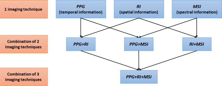
For the tissue classification process, the quadratic discriminant analysis (QDA) [10], a popular machine learning technique, is used. A post-processing methodology enhances global classification performance via a non-linear spatial filtering based on the mode of a small neighborhood [11,12]. The system has been tested on sample wounds performed on the back of a pig, by employing all possible combinations of the three available imaging techniques, as Fig. 1 represents. The performance has been validated through the application of a k-fold cross-validation. The results of this testing demonstrate that increasing the number of features improves the classifier performance.

Fig. 1.

Three independent optical imaging techniques collects the information of the subject: (a) temporal variation, (b) Spatial texture of the image, and (c) Multispectral reflection. The features if these techniques are combined in order to improve the accuracy of the tissue classification.

This paper is organized as follows: section 2 describes how the experiment with the pigs has been performed. Section 3 presents a summary of the PPG output processing (where the physiological information is obtained), a brief mathematical explanation of the QDA classifier, the definition of the features that involve each imaging technique, and the process for defining the Ground Truth (GT) images. Section 4 shows some classification and accuracy results, and it explains the mode filtering post-processing and the accuracy definition. In section 5, a discussion of the results is presented. Finally, the paper is concluded in section 6.

2. Description of the experiment

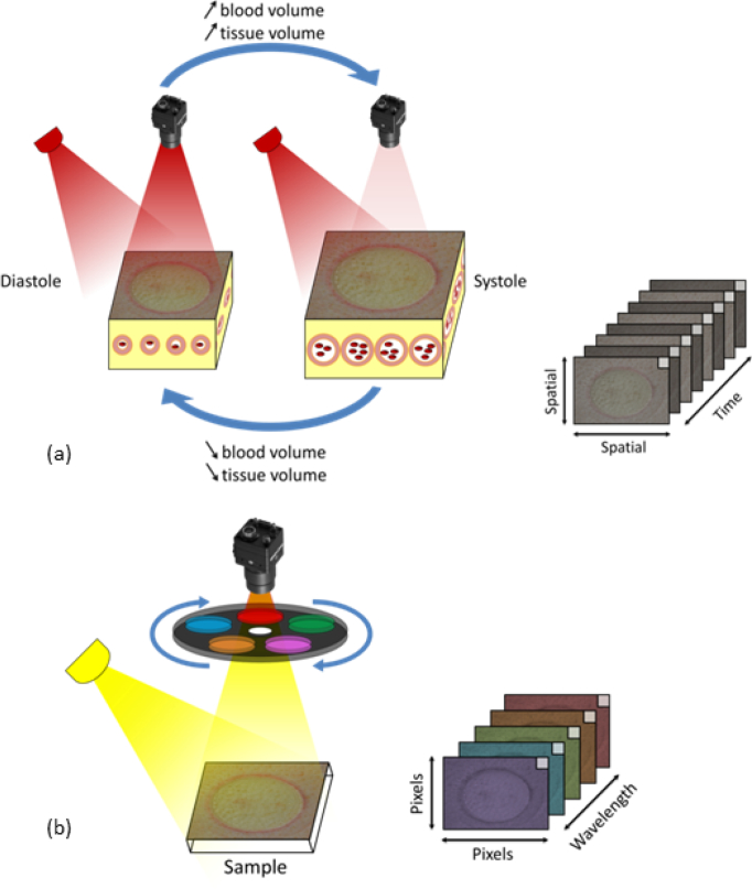
A porcine burn model of serial tangential excision was performed as described previously in [8,13,14]. In summary, an imager (CCD Sony, GE141) equipped with a filter wheel containing eight optical band-pass filters (400–1100 nm) was mounted coaxially to a custom built LED illumination array. The CCD has 1392 horizontal × 1040 vertical pixels and an active area of 10.2 mm × 8.3 mm. All data (PPG imaging, RI, and MSI data) is collected using the same sensor in 20–24 seconds. We assumed that the target is stationary, presenting minimal motion from frame to frame during this period; and, therefore, all data is considered to be intrinsically co-registered. Additional co-registration techniques may be required in the future for cases in which the stationary condition is not met anymore. Figure 2 shows schematically the process of data acquisition. Figure 2(a) depicts the PPG variation in time for a single frequency. The monocromatic light (λ = 850 nm) that incites on the tissue surface is scattered as it interacts with the molecular structures of the skin. The first frame is used for obtaining the RI information. Figure 2(b) shows the frequency response for the different light filters, which comprises the MSI data collection. Table 1 indicates the wavelengths of the eight MSI filters and their irradiance on the sample surface. The filter widths are ±10 nm. The spot size full width half maximum exceeds the field of view, which is 15 cm × 20 cm. The spatial variance in illumination of the target surface is less than 20%.

Fig. 2.

Optical data system: (a) Monochromatic light scattered from tissue. When measured over temporal interval, the intensity changes in the back-scattered light produce a PPG waveform; (b) Multispectral imager measures 8 wavelengths of light. This system quickly collects an image at each position to generate a spectral data cube [8].

Table 1.

Wavelengths of the MSI.

	Wavelength of MSI	Irradiance of LED on sample surface
λ 1	420 nm	3.1 · 102 μW/cm2
λ 2	525 nm	2.0 · 102 μW/cm2
λ 3	590 nm	9.0 · 101 μW/cm2
λ 4	620 nm	2.0 · 102 μW/cm2
λ 5	660 nm	2.9 · 102 μW/cm2
λ 6	720 nm	3.0 · 102 μW/cm2
λ 7	830 nm	1.2 · 103 μW/cm2
λ 8	850 nm	1.5 · 103 μW/cm2

Two adult Hanford swine were anesthetized and prepped for dorsolateral burns, which were generated by applying a pressure controlled brass rod (diameter 3.6 cm), heated to 100°C, to the skin for 45 seconds. Skin tone was uniform both across and between pigs. A total of six burns were created on each animal. An electric dermatome (Zimmer; Model No.:8821-06) set to 1 mm depth (width 6 cm) was passed over each burn sequentially, until the viable wound bed was exposed. This required three excisions to approximately 3–4 mm depth for all burns, and was confirmed immediately by punctate bleeding and later histology. Imaging with all three techniques was performed: pre-injury (healthy skin), immediately post-injury (acute burn), and after each layer was excised. A total of 80 minutes elapsed from the initial injury to the final excision.

3. Technical approach

3.1. PPG output pre-processing

The PPG images are created according to [15]. This pre-processing is carried out in order to obtain some physiological information related to the heart rate of the subject, which is used later as some initial features for the classification step.

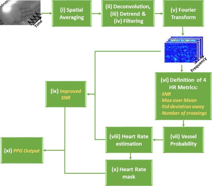
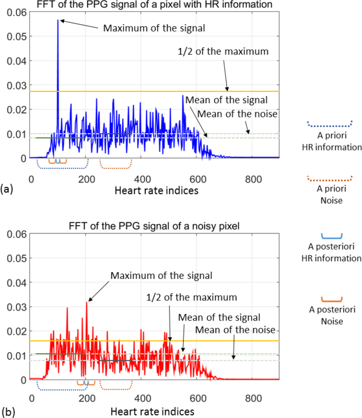
For each image, 800 frames are collected from a 27 second video of the burn wound. Then, a time variation PPG signal is defined for each pixel, in which a pre-processing algorithm is carried out, as schematized in Fig. 3 and summarized as follows: (i) An initial spatial averaging of all the frames is computed. (ii) Then, a deconvolution is performed, in which the high amplitude component at low frequency—corresponding to the artificial ventilation of the sedated pig—is removed. (iii) Next, a linear detrend of the signal applied. (iv) A range of frequencies, in which the heart rate is expected, is defined. A band-pass filtering is performed over this range. (v) In order to compute the frequency domain version, a Fast Fourier Transform (FFT) is applied to the time domain signal of each pixel. (vi) From these sets of frequency signals, four initial features are obtained, as they are explained as follows (two examples of these frequency signals and the graphical explanation of the computation of the metrics are shown in Fig. 4):

• 1.Signal to noise ratio (SNR), computed as the division between the mean of the signal defined over an a priori range in which the heart rate is expected (35 – 205 bpm) and the mean of the signal over an a priori range considered as noise (230 – 350 bpm);
• 2.maximum signal amplitude over its mean, computed as the ratio between the maximum of the signal and the mean of it;
• 3.number of standard deviations away from the mean, computed as the difference of the maximum and the mean of the signal divided by its standard deviation; and
• 4.number of crossings of the signal over one half of its maximum value.

Fig. 3.

Block diagram of the PPG Output preprocessing. In italics, the metrics obtained during this process.

Fig. 4.

Frequency representation (in terms of heart rates) of two PPG signals: (a) from a pixel with good HR information, (b) from a noisy pixel. The metrics of the first four features are calculated from the parameters described in the plot.

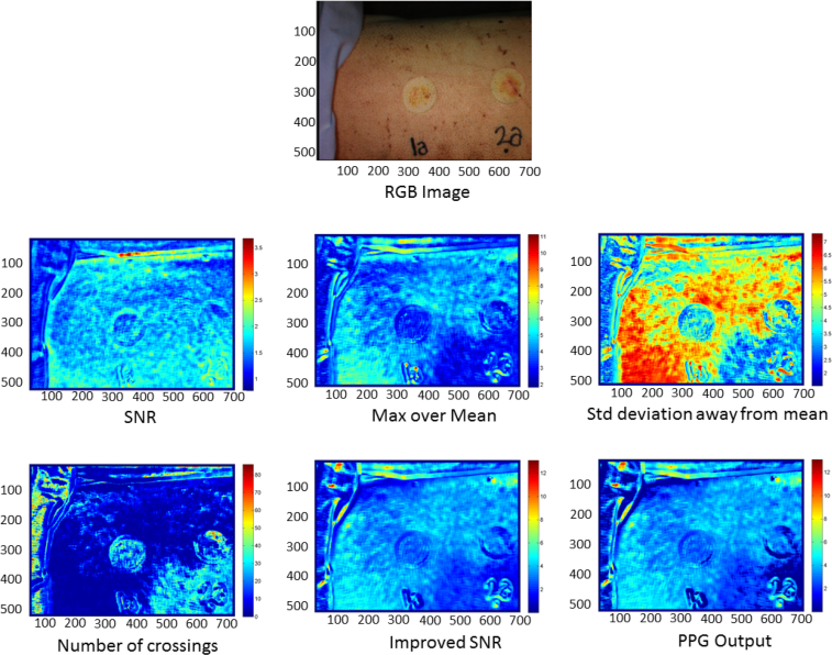
(vii) In order to determine if a pixel contains noise or good PPG signal (coming from a well perfused vessel), a linear discriminant analysis (LDA) was performed. The LDA coefficients for both the noise and good vessel signal were computed using data from previous experiments. A vessel probability is calculated as the softmax function of the scores obtained for the good vessel signal with respect to the noise. The vessel probability indicates how useful a pixel is for providing information about the heart rate of the subject. For the pixels whose vessel probability is greater than 0.9, the values of the heart rate (in bpm) corresponding to the maximum of the frequency signal are stored. (viii) The most repeated value is selected as the true heart rate of the pig under analysis. (ix) This value is used to obtain the improved SNR metric, which is calculated as the division of the mean of the signal defined on a posteriori range around the real heart rate (±2 bpm), between the mean of the signal defined on a posteriori range of values identified for the noise—a small range of ±15 bpm centered on the computed heart rate, excluding the range corresponding to the a posteriori heart beat rate.— (x) Finally, a mask is defined by setting to 1 those pixels whose heart rates correspond with the calculated rate, and setting to the remain of pixels a value between 0 and 1, depending on their degree of difference from the true heart rate. (xi) The PPG Output feature is the result of the product between the improved SNR and that mask. Figure 5 shows an example of the metrics of these six initial features for one of the injuries. These features give physiological information about the blood flow below the surface of the body of the subject under study.

Fig. 5.

Example of the RGB image and the six initial features of one injury.

3.2. Classification algorithm

Quadratic Discriminant Analysis (QDA) is a popular supervised classification algorithm for machine learning applications [10]. QDA is trained by assuming that the data follow a Gaussian distribution in n-dimensional space, where n is the number of features being used. Given the large amount of data available, the distribution of the features can be considered Gaussian, as per the central limit theorem.

QDA finds the type of class k that maximizes the conditioned probability P that a given pixel x belongs to that class k. Mathematically, the decision Ĝ(x) is given by the following expression:

$$\hat{G}(\mathit{x})=\underset{k}{\text{arg max}}P(G=k|X=\mathit{x})=\underset{k}{\text{arg max}}{f}_k(\mathit{x}){\pi }_k=\underset{k}{\text{arg max}}\left[{\delta }_k(\mathit{x})\right],$$ (1)

where δ_k(x) is called Quadratic Discriminant Function and is defined as follows:

$${\delta }_k(\mathit{x})=-\frac{1}{2}\text{log}\left|{\mathbf{\Sigma }}_k\right|-\frac{1}{2}{\left(\mathit{x}-{\mathit{\mu }}_k\right)}^T{\mathbf{\Sigma }}_k^{-1}\left(\mathit{x}-{\mathit{\mu }}_k\right)+\text{log}{\pi }_k.$$ (2)

The parameters that appear in Eqs. (1)–(2) are described as follows: the subscript k indicates the class of tissue and f_k (x) is the probability density function of an n–dimensional Gaussian distribution; μ_k and Σ_k represent the mean and the covariance matrix, respectively, for each class k; and π_k is the a priori probability for that class. The values of μ_k and Σ_k are calculated in the training step with a set of N known pixels defined by the pair (x, k), where x is an n–dimensional vector, which represents the values of each feature, and k is the class corresponding to that pixel. The value of N corresponds with all the pixels of the images used in the training step, and it is a value around 10⁷ pixels. For each class k, a value of δ_k(x), representing the likelihood that the unknown pixel x belongs to that class k, is obtained. The decision boundary between two classes k and l is defined as the set of pixels that satisfy {x : δ_k (x) = δ_l (x)}. Due to the definition of δ_k(x), this boundary is a quadratic function of x.

3.3. Definition of features

As outlined earlier, a set of features for each of the three imaging techniques have been defined to determine different properties of each pixel of the image under analysis. There are a total number of 33 features, distributed as follows: 14 features from the PPG Output process (six of them already explained in Sect. 3.1), 11 features from the RI, and 8 features from the MSI, one per each wavelength of light, as shown in Table 1. The description of each feature is shown in Table 2. The standard deviation, skewness, kurtosis, and the X and Y gradients features are computed with the provided Matlab functions std2, skewness, kurtosis, and gradient, respectively.

Table 2.

Description of all the features used in the experiment

PPG Output	Real image	Multispectral Images
1.PPG Output Image 2.Maximum over mean 3.Standard deviations away from mean 4.Number of crossings 5.SNR 6.Improved SNR 7.Lighting normalized 8.PPG image Normalized 9.Standard deviation 10.Skewness 11.Kurtosis 12.X-gradient 13.Y-gradient 14.Standard deviation of the gradients	1.Real image 2.Real image normalized 3.Skewness 4.Kurtosis 5.X-gradient 6.Y-gradient 7.Standard deviation within X-gradient 8.Standard deviation within a small neighborhood 9.Range within a small neighborhood normalized 10.Standard deviation within a big neighborhood 11.Range within a big neighborhood normalized	1.MSI λ1 2.MSI λ2 3.MSI λ3 4.MSI λ4 5.MSI λ5 6.MSI λ6 7.MSI λ7 8.MSI λ8

3.4. Definition of ground truth images

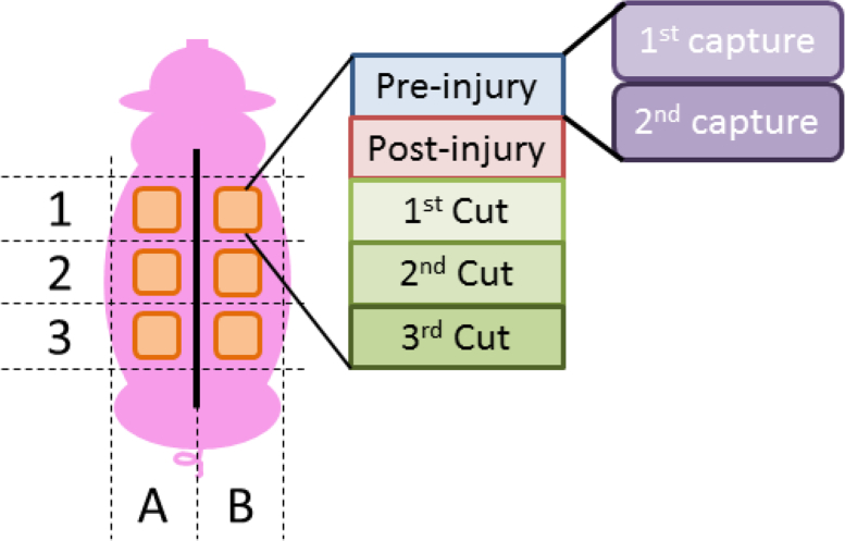
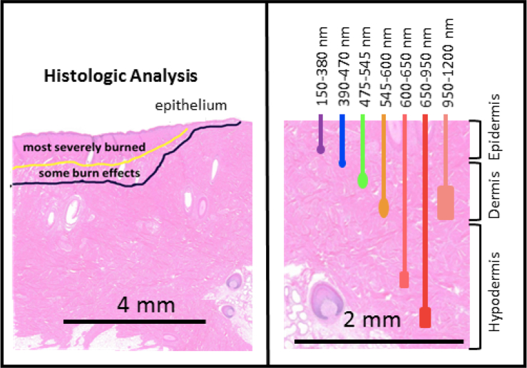
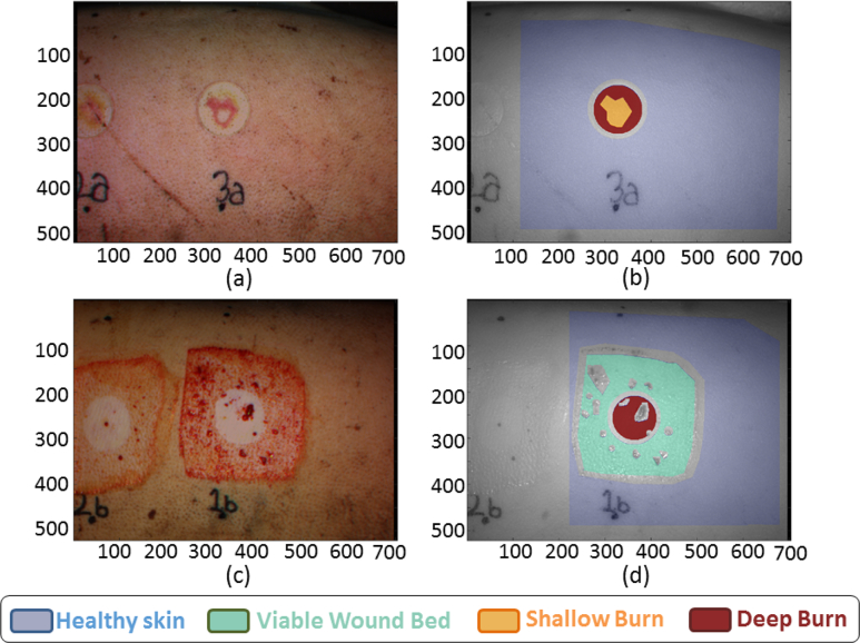
Since QDA is a supervised learning classifier, some control data need to be provided to train the algorithm. Therefore, a database of Ground Truth (GT) images for all the cases under study was generated. For the analysis of one pig, a total number of 60 cases are available, described as follows: six lesion locations (three at each side of the back of the pig) for five stages (pre-injury, post-injury, first excision, second excision, and third excision), with two imaging captures taken at each stage, as it can be seen in Fig. 6. These control data have been generated by analyzing each injury site and deciding the type of tissue for each area of the image. These decisions have been taken by an specialist, based on the histologic analysis, as shown in Fig. 7, [8, 16, 17]. The different wavelengths have a different range of penetration in the skin, as seen in Table 3 [4,17,18], helping to identify the depth of the burns. The image data are then separated into classes, corresponding to each tissue type. A total of four different classes have been defined: healthy skin, viable wound bed, deep burn, and shallow burn tissues. The GT matrices define the different kinds of tissue in each capture. Some sets of pixels out of the region of interest, such as areas with hair, marked with ink, or regions between tissues classes, were discarded. This prior definition of the tissues is used in the classification algorithms, since they represent the ideal output of the classifier. Examples of the transition from the real image to the GT are shown in Fig. 8.

Fig. 6.

Location of the injuries on the back of the pig.

Fig. 7.

The left side represents a partial thickness burn showing the histologists markings on the tissue. The right side shows the penetration in the skin for different wavelengths of light.

Table 3.

Penetration in skin for different wavelengths

Wavelength (nm)	Color Range	Penetration (mm)
150 – 380	UV	< 0.1
390 – 470	Violet to Deep Blue	∼ 0.3
475 – 545	Blue–Green	∼ 0.3 – 0.5
545 – 600	Yellow to Orange	∼ 0.5 – 1.0
600 – 650	Red	∼ 1.0 – 2.0
650 – 950	Deep Red–NIR	2 – 3
950 – 1200	NIR	1

Fig. 8.

(a) Real image and (b) Ground Truth of the post-injury case 3A1. (c) Real image and (d) Ground Truth of the first excision case 1B1.

4. Results

The total available data consist of 12 sets, corresponding to six locations and two imaging captures per location for one pig. Each set contains the data of the five stages of the injury process performed at each location: pre-injury, post-injury, and first, second, and third excision. The k-fold cross-validation for a value of k = 12 (leave-one-out) has been performed in order to validate the imaging techniques. This validation method consists on dividing the whole data in k folds and, one by one, leave one of the folds for classification and use the remain folds for training, computing the imaging and accuracy results [10]. The mean and standard deviation of the k accuracy values are calculated in order to assess the performance of the model. The definition of the accuracy metric used for evaluating the performance of the classifier is defined later in this section.

The study has been applied seven times, by varying the set of features used for each imaging technique, as indicated in Table 4. For graphical purposes, two examples are depicted: the first capture of the post-injury step in location 3A, and the first capture of the first excision step in location 1B. Figure 8 shows the real image and the GT—which is considered as the reference to compare with the later classification images—of these examples, as well as the color code.

Table 4.

Number of features used for each imaging technique

Imaging Technique	# of features
PPG	14
RI	11
PPG+RI	25
MSI	8
PPG+MSI	22
RI+MSI	19
PPG+RI+MSI	33

It is expected an enhancement on the accuracy results when the imaging techniques are combined. A regular classification and a classification using a non-linear post-processing method are compared in this section in order to evaluate further improvements in the accuracy results.

4.1. Regular classification

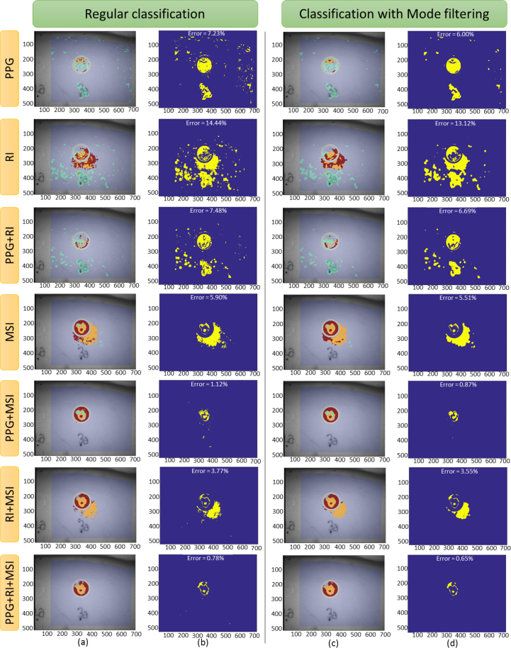
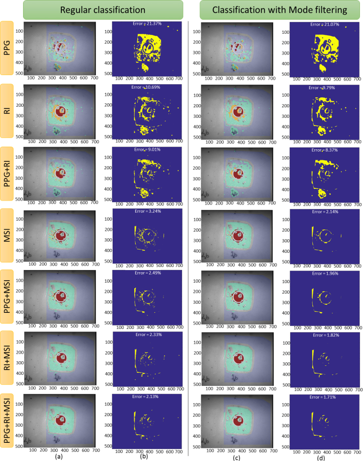
Making use of all the data available, the 12-fold cross-validation, by using QDA with equal a priori probability (${\pi }_k=\frac{1}{4}$), has been applied. Figures 9(a)–(b) show the classification results, the image error, and the percentage of error, for each imaging technique, in the first example (3A1). In the same way, Figs. 10(a)–(b) show the equivalent results for the second example (1B1).

Fig. 9.

(a)–(b) Regular classification and (c)–(d) classification after applying the mode filtering post-processing, for the post-injury step of the case 3A1. Each row plots the results using the features of the indicated imaging technique. (a) and (c) columns plot the classification image, and (b) and (d) columns plot the classification error (blue color indicates correct classification and yellow indicates wrong classification), indicating, as well, the total error of classification.

Fig. 10.

(a)–(b) Regular classification and (c)–(d) classification after applying the mode filtering post-processing, for the first cut step of the case 1B1. Each row plots the results using the features of the indicated imaging technique. (a) and (c) columns plot the classification image, and (b) and (d) columns plot the classification error (blue color indicates correct classification and yellow indicates wrong classification), indicating, as well, the total error of classification.

Based on the results of the classifier, a confusion matrix was constructed for each case. An example of this matrix, based on the classification made with all the 33 features, is shown in Table 5. The parameters included in confusion matrices are defined after the table.

Table 5.

Example of a confusion matrix

		GT class
		Healthy skin	Viable Wound Bed	Shallow Burn	Deep Burn
Assigned class	Healthy skin	R = 0.9874	R = 0.0329	R = 0.0142	R = 0.0102
		r = 0.9945	r = 0.0053	r = 0.0000	r = 0.0001
		C = 0.8381	C = 0.0045	C = 0.0000	C = 0.0001
		e = −0.0070	e =0.0275	e =0.0142	e = 0.0100
	Viable Wound Bed	R = 0.0123	R = 0.9494	R = 0.2987	R = 0.0875
		r = 0.0734	r = 0.9139	r = 0.0056	r = 0.0071
		C = 0.0104	C = 0.1301	C = 0.0008	C = 0.0010
		e = −0.0611	e = 0.0355	e = 0.2931	e = 0.0804
	Shallow Burn	R = 0.0000	R = 0.0143	R = 0.4753	R = 0.0211
		r = 0.0016	r = 0.5628	r = 0.3661	r = 0.0696
		C = 0.0000	C = 0.0020	C = 0.0013	C = 0.0002
		e = −0.0016	e = −0.5485	e =0.1092	e = −0.0485
	Deep Burn	R = 0.0003	R = 0.0034	R = 0.2118	R = 0.8812
		r = 0.0194	r = 0.0409	r = 0.0499	r = 0.8898
		C = 0.0002	C = 0.0005	C = 0.0006	C = 0.0101
		e = −0.0191	e = −0.0375	e = 0.1619	e = −0.0086

• R: reconstruction rate, defined as the probability that a pixel is classified into one assigned class, when it belongs to a given GT class, P(assigned class / GT class). It is also known as Sensitivity,

• r: recognition rate, defined as the probability that a pixel belongs to a given GT class, when it has been classified into one assigned class, P(GT class / assigned class). It is also known as Precision,

• C: combination rate, defined as the probability that a pixel belongs to a given GT class and is classified into one assigned class, P(GT class ∩ assigned class),

• e: estimation index, defined as the difference between the reconstruction and the recognition rates.

The reconstruction and recognition rates are values between 0 and 1, indicating weak or strong performance, respectively. For a perfect classifier, R and r are 1 in the main diagonal and 0 in the off–diagonal entries of the matrix; and, in the same way, the estimation index e is 0 in all entries of the matrix. In any case, probability axioms make the summation of all combination rate values C to be equal to 1. For evaluating a real classifier, the closer the values of R, r, and e are to those of the perfect classifier, the better performance.

In order to quantitatively determine the performance of the classification, an accuracy parameter is defined. From the diagonal of the confusion matrix, the accuracy per class A_i is defined as the geometric mean of the reconstruction and recognition rates, as follows:

$$A_i=\sqrt{R_i\cdot r_i},$$ (3)

where the subindex i indicates the class. This accuracy index rewards high simultaneous sensitivity and precision, while penalizing large differences between them. The global accuracy A of the classifier is computed as the arithmetic mean of the accuracy of the N_C classes:

$$A=\frac{1}{N_C}\sum _{i=1}^{N_C}{A}_i,$$ (4)

Table 6 shows the accuracy values for each class and the global accuracy of the experiment for each of the seven combinations of imaging techniques. Since the 12-fold cross-validation method was applied, each value in the table corresponds to the mean of all cross-validations for the specific case. It can be noticed that the global accuracy is increased by 80% when combining all the imaging techniques, that is, when using all the features, with respect to the use of only the PPG features.

Table 6.

Accuracy mean comparison when combining different imaging techniques

Set of features	Healthy Skin	Viable Wound Bed	Shallow Burn	Deep Burn	Global
PPG	0.8461	0.4728	0.0823	0.2173	0.4272
RI	0.9158	0.7135	0.2512	0.4461	0.6023
PPG+RI	0.9298	0.7433	0.2190	0.4675	0.6120
MSI	0.9746	0.9418	0.3856	0.5543	0.7336
PPG+MSI	0.9835	0.9417	0.3797	0.6383	0.7552
RI+MSI	0.9783	0.9216	0.3833	0.6726	0.7603
PPG+RI+MSI	0.9825	0.9212	0.3918	0.6979	0.7689

4.2. Classification after mode filtering post-processing

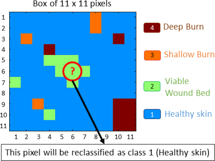
Due to the particular characteristics of the image classification, a spatial post-processing may be applied. It is reasonable to think that the classification in a small neighborhood should not have a lot of variability. A non-linear spatial filtering based on the mode (the most repeated value) of a small neighborhood has been applied, [11, 12]. Since there are only four possible classes, each pixel of the image has been redefined, after the regular classification, as the mode of an 11 × 11 square centered on it. This post-processing method is graphically explained in Fig. 11. The classification results of the previous examples are shown in Figs. 9(c)–(d) and Figs. 10(c)–(d). Table 7 shows the accuracy results per class and the global accuracy for the seven different classification methods, depending on the set of features selected for the training, when applying the mode filtering post-processing after the regular classification.

Fig. 11.

Graphical example of the application of the mode filtering post-processing. The pixel in the middle of the image is reclassified as the most repeated value of the 11 × 11 box.

Table 7.

Comparison of the accuracy mean when combining different imaging techniques, plus the use of the mode filtering post-processing

Set of features	Healthy Skin	Viable Wound Bed	Shallow Burn	Deep Burn	Global
PPG	0.8774	0.5157	0.0815	0.2310	0.4456
RI	0.9227	0.7385	0.2744	0.4627	0.6198
PPG+RI	0.9376	0.7708	0.2225	0.4982	0.6305
MSI	0.9754	0.9493	0.4266	0.5653	0.7472
PPG+MSI	0.9853	0.9510	0.4280	0.6642	0.7749
RI+MSI	0.9803	0.9289	0.4005	0.6968	0.7726
PPG+RI+MSI	0.9847	0.9289	0.3959	0.7209	0.7784

5. Discussion

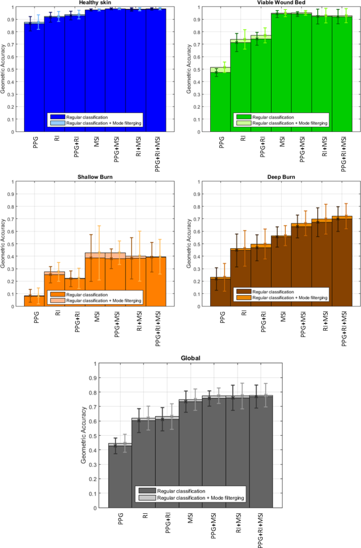
Figure 12 plots the accuracy comparison of each class and the global accuracy when the classification is done using the features of the indicated imaging technique. The performance of the classification after applying the mode filtering post-processing is plotted with lighter color bars. Error boxes indicate ±1 standard deviation of the results with respect to the mean values. By introducing the MSI features, the classification accuracy is greatly boosted with respect to the case when only PPG and RI features are used. The accuracy is notably improved when combining all the available features. These results are further enhanced after applying the above-mentioned mode filtering post-processing. Table 8 shows the relative improvement of the mean accuracy values when applying the mode filtering post-processing, compared to the regular classification.

Fig. 12.

Accuracy per class and global accuracy of the performance, based on the set of features used for classification. The lighter colors indicate the improvement after applying the mode filtering post-processing. Error boxes indicate ±1 standard deviation from the mean values.

Table 8.

Accuracy improvement after applying the mode filtering post-processing, relative to the regular classification

Set of features	Healthy Skin	Viable Wound Bed	Shallow Burn	Deep Burn	Global
PPG	1.54 %	9.07 %	−0.97 %	6.30 %	4.31 %
RI	0.75 %	3.50 %	9.24 %	3.72 %	2.91 %
PPG+RI	0.84 %	3.70 %	1.60 %	6.72 %	3.02 %
MSI	0.08 %	0.80 %	10.63 %	1.98 %	1.85 %
PPG+MSI	0.18 %	0.99 %	12.72 %	4.06 %	2.61 %
RI+MSI	0.20 %	0.79 %	4.49 %	3.60 %	1.62 %
PPG+RI+MSI	0.22 %	0.84 %	1.05 %	3.30 %	1.24 %

This non-linear filtering reduces all small misclassifications, as shown in Figs. 9(c)–(d) and 10(c)–(d) when compared to Figs. 9(a)–(b) and 10(a)–(b), respectively, increasing the accuracy per class and the global accuracy. On the contrary, if the original classification is not effective, some isolated, well-classified pixels within a wrongly classified area could be removed, reducing the classification accuracy. The negative entry in Table 8 indicates this fact. It can be noticed how the healthy skin tissue is well identified in the regular classification; therefore, the improvement achieved after applying the mode filtering post-processing is not significant. Moreover, the small standard deviation in this tissue indicates stable classification. In contrast, the shallow burn tissue is more difficult to detect and it has a huge variability, meaning that the classification is not reliable. Generally, the application of the mode filtering improves the accuracy results of this tissue. Finally, the performance in the deep burn tissue, which may be considered as the most important tissue to identify, and the global performance are enhanced when new features are added. Also, the application of the mode filtering post-processing improves the results in these two cases. The standard deviation remains within a range of [0.08, 0.12] for deep burn and [0.05, 0.09] for global, for all the experiments once MSI features are introduced, indicating a good general performance of the classifier.

6. Conclusion

It has been shown that the proposed imaging system is capable of distinguishing burn tissue among other types of tissues with the information provided by the features of three different optical imaging techniques: PPG, RI and MSI. A QDA classifier model has been adopted to successfully complete this task. A definition of the accuracy based on the geometric mean of the sensitivity and the precision has been presented. This paper has shown the performance of the 12-fold cross-validation algorithm when the imaging techniques are combined, that is, when the number of features is increased. Moreover, the introduction of the MSI features has improved the accuracy of tissue classification by 80%. Furthermore, the application of the mode filtering post-processing has improved the accuracy of the classification when the original performance is satisfactory, smoothing the transitions between areas and removing small misclassifications. Example of classification plots and a confusion matrix, numerical tables with the accuracy per tissue and global accuracy, as well as graphics showing the evolution of the accuracy per tissue and the global accuracy, have been presented in this paper. Further developments will continue to increase the sensitivity and accuracy of the imaging system through pre-processing of the training data, adding more features, or applying other post-processing techniques. A transition from imaging pig burns to real-world human burns is currently under investigation, in order to fully test and ultimately implement a non-invasive, low-cost, automated burn detection system.

Funding

Biomedical Advanced Research and Development Authority (BARDA) (HHSO100201300022C).

Disclosures

The authors declare that there are no conflicts of interest related to this article.