Feature-based Representation Improves Color Decomposition and Nuclear Detection Using Convolutional Neural Network

Abstract

Detection of nuclei is an important step in phenotypic profiling of (a) histology sections imaged in bright field; and (b) colony formation of the 3D cell culture models that are imaged using confocal microscopy. It is shown that feature-based representation of the original image improves color decomposition and subsequent nuclear detection using convolutional neural networks (CNN)s independent of the imaging modality. The feature-based representation utilizes the Laplacian of Gaussian (LoG) filter, which accentuates blob-shape objects. Moreover, in the case of samples imaged in bright field, the LoG response also provides the necessary initial statistics for color decomposition (CD) usings non-negative matrix factorization (NMF). Several permutations of input data representations and network architectures are evaluated to show that by coupling improved color decomposition and the LoG response of this representation, detection of nuclei is advanced. In particular, the frequencies of detection of nuclei with the vesicular- or necrotic-phenotypes, or poor staining are improved. The overall system has been evaluated against manually annotated images, and the F-scores for alternative representations and architectures are reported.

I. Introduction

Cellular organization is an important index for profiling diseased regions of microanatomy and aberrant colony formation in 3D cell culture models. In histology sections, the normal cellular organization is often lost as a result of rapid cellular proliferation in tumors. For example, the degree of cellularity is one of the indices for (i) diagnosis of Glioblastoma Multiforme (GBM) as a result of increased proliferation of glial cells, (ii) evaluating the efficacy of a neoadjuvant chemotherapy of breast carcinoma [1], (iii) characterizing pleomorphic nuclear phenotypes in breast cancer [2], and (iv) grading prostate cancer-based Gleason score [3]. In the 3D cell culture model of malignant human mammary epithelial cells, normal spherical colony formation is often transformed to sheet-like structures with increased cellularity. Furthermore, regardless of 2D or 3D sample preparation and imaging, cellularity can also be heterogeneous, which is potentially the result of cellular plasticity. The goal of this paper is to develop validated computational tools for detection of nuclei that enable quantification of cellularity either from a large cohort of hematoxylin and eosin (H&E) stained histology sections, imaged in bright field, or 3D colony formation assays are imaged with confocal microscopy. However, a large cohort of H&E stained histology sections often suffers from technical and biological variations where a number of methods have been proposed in the context of nuclear segmentation [4], [5]. Here, technical variations refer to variations in fixation and staining, and biological heterogeneity refers to the fact that no two patients are alike and that local and global patterns of diseased tissues vary widely. The novelty of this paper is two folds with the common thread that the LoG response can improve color decomposition (CD) and nuclear detection. In the first case, the LoG filter provides the necessary initial statistics for color decomposition using non-negative matrix factorization (NMF). In the second case, the LoG filter enhances significant spatial distribution of the underlaying image to improve nuclear detection using CNN. However, for H&E stained sections, improved color decomposition also improves the accuracy of nuclear detection using CNN.

One of the limitations of the NMF is that random initialization provides unstable CD, and repeated applications of NMF provide different color decompositions. The rationale being that NMF is essentially a greedy approach and is sensitive to initialization. However, with proper initialization based on image statistics corresponding to peaks and valleys of the LoG filter response, a more stable CD is computed. This technique is referred to as NMF(LoG), which has also shown to have a superior performance profile when compared to other techniques. With respect to the nuclear detection with CNN, samples can be represented either as 2D or 3D images and the network architecture can be either shallow or deep. Both shallow and deep CNN have been trained with different permutations of input data representation for both 2D and 3D data. Evaluation is performed against a large set of manually curated images.

Organization of this paper is as follows: Section II reviews previous research. Section III describes the details of the proposed color decomposition, network configuration, and input feature representations. Section IV presents our experimental results and performance of alternative architectures. Lastly, Section V concludes the paper.

II. Background

The topics of nuclear detection and segmentation have been widely explored in 2D and 3D images [6], [7], [8], [9], [10], and a very recent review paper summarizes alternative methodologies for nuclear detection and segmentation [11]. Traditionally, nuclear detection strategies have relied on either model-free or model-based techniques. These include variations of seed detection based on morphological operators and distance transform [12] [13], iterative voting [14], and fast radial transform [15], [16]. However, more recently, convolutional neural networks (CNN) [17] have also been extended for nuclear detection where CNNs are trained for a specific pattern to elucidate a model automatically. Several configurations of CNN have been suggested for detection of nuclei in histology images, and two cases are summarized below. In [18], a model of CNN has been proposed to learn the localization and its corresponding confidence values jointly; however, the method has been tested on samples that have been stained with the Ki-67, a proliferating marker, and the experimental design can benefit from a different marker since Ki-67 and the nuclear stain are co-localized and have an additive signal. In [19], a spatially constrained model of the CNN has been proposed for nuclear detection where the constrain is based on a pre-defined distance measure. Detection of nuclei, using CNN, imposes a challenge as a result of having a single response (e.g., a delta function) for each nucleus, and one cannot train a CNN with such an input-output response. Therefore, a real-valued spatial landscape needs to be defined for training.

The differences between our approach and previous methods are 3 folds. Previous researchers have (I) validated their method with samples that came from one laboratory; hence strict quality control for sample preparation has been enforced; (II) not evaluated the effects of color decomposition and the presence of multiple nuclear phenotypes; (III) not evaluated nuclear detection in 3D samples that have been imaged with confocal microscopy. More importantly, we train the CNN with the LoG response of the image following accurate color decomposition. The LoG response is advantageous over the various distance functions that have been proposed in the past. The LoG response captures intrinsic spatial landscape for each nucleus; hence, no artificial distance function is needed to encode the input-output relationships in the CNN. In other words, the LoG response captures pertinent information about the nuclear shape and size with the outcome being an improved performance.

III. Methods

A. Color Decomposition for H&E Stained Sections

In this section, we focus on H&E stained tissue sections that are visualized in the RGB color space. In this assay, hematoxylin and eosin stain the DNA and the protein macromolecules in blue and pink colors, respectively. However, two problems persist: in most cases, (i) there are variations in tissue fixation and staining that lead to a significant batch effect; and (ii) biological heterogeneity persists per patient and across patients. The latter can be caused by either macromolecules being secreted into the tumor microenvironment as a result of cellular stress, heterogeneous response to therapy, or presence of mixed tumor types. Often these two problems are interrelated in a large cohort; thus, color decomposition needs to be adjusted per histology section or per field of view. Although a number of methods have been proposed for color decomposition, we aim to extend non-negative matrix factorization (NMF) [20], [21].

NMF is a matrix factorization method that assumes an image can be decomposed into parts and subparts, and that image composition from its parts is strictly non-negative. This is an appropriate model for CD since each stain uniquely adds to the components of the color space. Typically, in NMF, basis and coefficient matrices are randomly initialized and the solution is optimized by iteratively fixing one variable and estimating the other one. This approach is intrinsically a greedy search method that with poor initialization may lead to an undesirable solution, i.e., different initializations lead to different deconvolutions matrices. Furthermore, poor initialization may also lead to a random ordering of nuclear and non-nuclear channels. One promising method for initialization is peaks associated with the response of the LoG filter since nuclei have a blob-like morphometry and are darker than the background. Accordingly, the LoG filter is used to generate the initial statistics. However, optical density transformation is a necessary requirement prior to the application of NMF. Optical density linearizes the relationship of the color distribution in the RGB space, as shown Figure 1. Hence, the steps are:

Fig. 1.

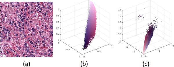
Optical density representation linearizes color separation of the RGB space. (a) The original image, (b) scatter plot in the RGB space, and (c) scatter plot in the optical density space.

1) Optical Density transformation

Let S ∈ R^3×2 be the mixing matrix, and M ∈ R^2×N, where N is number of pixels of the image. Then the Beer-Lambert law [22], for stain absorption of light, satisfies the following equation:

$$I=I_0{e}^{-SM}$$ (1)

Where I is the RGB image, I₀ is the maximum value of I in all channels, and matrices M and S are to be estimated. However, the non-linear Equation 1 can be linearized simply by:

$$SM=-\mathit{log}(\frac{I}{I_0})$$ (2)

The optical density (OD) is then defined as the product of stain and coefficient matrices or:

$$D=SM$$ (3)

Where D is the OD transform of RGB image I. This representation is shown in Figure 1 a–c, where the OD representation (i) linearizes color separation in the RGB spaces, and (ii) facilities color decomposition via matrix factorization techniques.

2) NMF Initialization

Color decomposition using NMF requires estimation of matrices M (coefficient matrix) and S (stain matrix) of the following equation. While the coefficient matrix is randomly initialized, the stain matrix is initialized according to the intrinsic properties of the image.

In order to generate the statistics for the initial stain matrix, a prior model is constructed by computing the peaks that correspond to the LoG response of the blue channel in the RGB image. Ideally, positive and negative peaks correspond to the foreground (e.g., nuclei) and background regions, respectively. In practice, there can be a significant amount of overlap [4]. Therefore, a probability distribution function is constructed, and a percentage of the top and bottom peak candidates is selected. This particular threshold (e.g., percentage) simply selects conservative peaks that strictly belong to nuclei and non-nuclei regions. Subsequently, these peaks are projected onto the RGB channel where the pixel intensities are read and averaged per image to establish the initial conditions. Algorithm 1 illustrates the required steps to calculate the initial stain matrix.

Algorithm 1.

Stain Matrix Initialization

Input: Blue channel of RGB image

Output: Stain matrix M3×2

Step 1: Compute LoG response of the input

Step 2: Compute local peaks of the LoG response

Step 3: Compute the density distribution of the peaks

Step 4: Select a conservative representative subset of minimum (e.g., negative values) and maximum (e.g., positive) peaks from the density distribution

Step 5: Average RGB values of minimum and maximum peaks of Step 4 to set the initial stain matrix

B. Nuclei Detection

Detection of nuclei is performed by using a CNN as a classifier and applying sliding window through the whole image. The result will be a probability map, which indicates the probability of each pixel to be the centroid of a nucleus.

Typically, a CNN consists of a cascade of layers which map an input image x to output vector y. Each layer is represented as (f₁, f₂, …, f_L), and the input-output relationship is given by:

$$\begin{array}{l}y=f\left(x;w_1,w_2,\dots ,w_L\right)\\ =f_L\left(.,w_L\right)\circ f_{L-1}\left(.,w_{L-1}\right)\circ \dots \circ f_1\left(x,w_1\right)\end{array}$$

Where each w_i is the bias and the weight for f_i in the ith layer; f_is are defined as functions of layers (e.g., convolution, max-pooling) with a specific activation policy (e.g., sigmoid, tanh, ReLU) at that layer; the weights and biases (w_is) for each layer are learned with an annotated dataset; and a loss function minimizes the output of network against the input data. This loss function, shown below, is minimized using the stochastic gradient decent technique.

$$\begin{array}{r}\underset{w_1,\dots ,w_L}{\mathrm{argmin}}\frac{1}{N}{\displaystyle \sum _{i=1}^{N}L\left(f\left(x^i;w_1,\dots ,w_L\right),y^i\right)}\\ +{\displaystyle \sum _{l=1}^L\left({\mathrm{\lambda }}_{1l}{\Vert w_l\Vert }_1+{\mathrm{\lambda }}_{2l}{\Vert w_l\Vert }_2\right)}\end{array}$$

In the remainder of this section, we examine variations in the representation of input data and network architectures.

There are mutiple polices for preprocessing of the input data. In the case of histology sections, preprocessing of the input representations can be enumerated as a function of RGB, grayscale, LoG response of the blue channel, NMF, and LoG response of NMF corresponding to the nuclear channel. In the case of 3D fluorescence images, representations can be enumerated as a function of gray scale or LoG of the gray scale. The selection policy of the input patch, for training the CNN, is also evaluated as a function of random selection or strictly nuclei-centered regions.

Gray or RGB normalized images have been widely used for training CNN; however, nuclei detection can benefit from the LoG response that accentuates their blob-shape property. Nevertheless, there are several permutations of the input representation with the LoG filter that need to be evaluated. For example, one can apply the LoG filter to the gray level representation of the original image or to the nuclear channel following color decomposition by NMF.

With respect to the patch selection for training the CNN, there are two dominant strategies that include either random patch selection or selection of nuclei centered patches. In the former, data augmentation is less significant because random selection can intrinsically increase the sample size. In the latter case, data augmentation is highly desirable and necessary. Strategies for data augmentation include affine transform, perturbations of the appearance model by manipulating computed basis functions, and elastic deformation.

2) Variations in the Network Architecture

There are many permutations of the CNN architecture (e.g., in terms of convolution size, size of the filter bank, activation function, contrast enhancement), but the dominant differences are shallow versus deep networks. Thus, different network configurations have been designed to evaluate the best performing architecture. Several variations of shallow and deep CNN have been evaluated, where the deep CNN is based on VGG [23]. With respect to the shallow CNN, two convolutional layers with 2 × 2 max-pooling and ReLU as an activation function provided the better performance. This network is shown in Figure 2. The last stage has a LogSoftmax function that computes the probability of each pixel as being the centroid of the nuclei. Table I indicates the design of the shallow CNN (ShCNN) for a 2D image (histology).

Fig. 2.

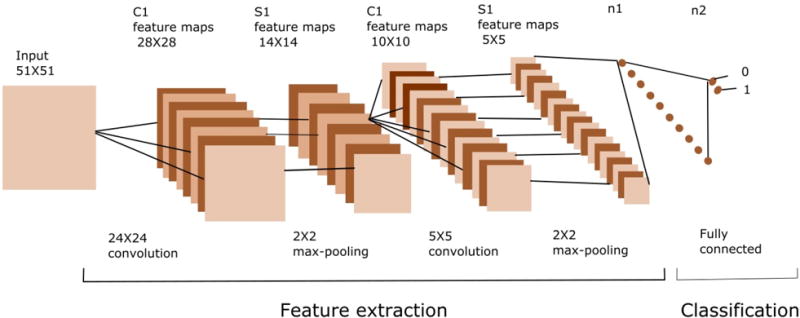
A CNN is made of two basic parts which are feature extraction and classifier. Feature extraction includes several convolution layers followed by max-pooling and an activation function. The classifier usually consists of fully connected layers.

TABLE I.

Shallow CNN with two layers of convolution

Layer	Type Input/Output	Dimensions	Filter Dimensions
0	Input	51 × 51 × 1
1	Conv	28 × 28 × 256	24 × 24 × 1 × 256
2	Max-Pooling	14 × 14 × 256	2 × 2
3	Conv	10 × 10 × 128	5 × 5 × 256 × 128
4	Max-Pooling	5 × 5 × 128	2 × 2
5	Full	1 × 2	–
6	LogSoftmax	–	–

With respect to the deep networks (e.g., VGG architecture), eight layers with 3 × 3 convolutions were constructed. The output classifier consists of two fully connected layers, and the log probability is computed using the LogSoftmax function. The dropout technique [24] has been applied in the last two layers in order to avoid over-fitting. Specifications of the deep convolutional neural network (DCNN) are indicated in Table II. Finally, with respect to the detection of nuclei imaged with confocal microscopy, the network architectures are identical to those designed and tested for 2D histology images with the exception that all convolutions are performed in 3D.

TABLE II.

DCNN with eight layers of convolution

Layer	Type Input/Output	Dimensions	Filter Dimensions
0	Input	51 × 51 × 1
1	Conv	48 × 48 × 64	4 × 4 × 1 × 64
2	Conv	46 × 46 × 64	3 × 3 × 64 × 64
3	Conv	44 × 44 × 64	3 × 3 × 64 × 64
4	Max-Pooling	22 × 22 × 64	2 × 2
5	Conv	20 × 20 × 128	3 × 3 × 64 × 128
6	Conv	18 × 18 × 128	3 × 3 × 128 × 128
7	Conv	16 × 16 × 128	3 × 3 × 128 × 128
8	Max-Pooling	8 × 8 × 128	2 × 2
9	Conv	6 × 6 × 512	3 × 3 × 128 × 512
10	Conv	4 × 4 × 512	3 × 3 × 512 × 512
11	Max-Pooling	2 × 2 × 512	2 × 2
12	Full	512	–
13	Dropout	–	–
14	Full	128	–
15	Dropout	–	–
16	Full	2	–
17	LogSoftmax	–	–

IV. Evaluation

This section evaluates the proposed techniques for color decomposition, nuclear detections in 2D and 3D, sensitivity analysis, strategies in training, over-fitting analysis, and the effect of boosting on the overall performance. Two datasets have been curated for nuclear detection in 2D (e.g., histology) and 3D samples (e.g., cultured multicellular systems) that are imaged with brightfield and confocal microscopy, respectively. Annotated histology sections consist of 29 images of brain and breast cancer tumor sections, with a total of 13,766 annotated nuclei. Annotated multicellular systems consist of 68 samples, where each sampled is imaged at 0.25 micron resolution in the XY directions and 1 micron resolution in the Z direction resulting in images of approximately the size of 256-by-256-by-80 pixels. In both cases, samples were equally divided for training and testing. More specifically, (i) in the case of 2D, 15 images were used to generate 200,000 data points for training through random selection or data augmentation, and (ii) in the case of 3D, 34 images were selected to generate 8000 data points for training through random selection. The rest of the data were used for testing.

A. Color Deconvolution

The effectiveness of the color deconvolution approach is compared against (i) NMF[27] with random initialization, (ii) the classical method proposed by Ruifrok and Johnston[28], (iii) the method based on singular value decomposition proposed by Macenko et al [26], and (iv) the method proposed by Khan et al[25]. Implementation of the last two methods are borrowed from the stain normalization toolbox [29], and evaluation is based on the quality of segmentation computed by applying the Otsu thresholding method. The performance of color decomposition is quantified in terms of F-Score, precision, and recall. Table III shows superior performance of the proposed method against prior state of art. Figure 3 illustrates the qualitative results of color deconvolution of Khan et al.[25], Macenko et al.[26], and the proposed method, respectively.

TABLE III.

Performance Evaluation of Alternative Color Decomposition Strategies

Method	Precision	Recall	F-Score
Proposed	0.7302	0.6548	0.6904
NMF	0.7215	0.6170	0.6651
Ruifrok and Johnston.[28]	0.5951	0.6891	0.6386
Macenko [26]	0.7746	0.6025	0.6568
Khan [25]	0.7408	0.5428	0.6265

Fig. 3.

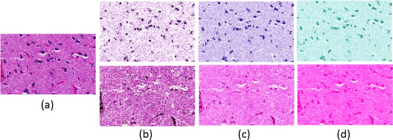
Each column shows color deconvolution results by different methods in the original color map space. (a) Original image, (b) Khan [25], (c) Macenko [26], (d) NMF(LoG) (proposed).

B. Detection of Nuclei from the 2D Histology Images

In order to evaluate the proposed concept, multiple configurations are implemented and the performance is quantified. These configurations include input representation (e.g., raw versus engineered features), network architecture (e.g., deep versus shallow networks), and patch selection for training (e.g., random patches, nuclei centered patches). The batch gradient descent with a batch size of 256 is used for back propagation optimization. The learning rate is set at 10⁻⁵ and the learning rate decay is set at 10⁻⁷. L₁ and L₂ regularizations were performed with weights of 0.001 and 0.01, respectively. Since proper initialization is critical for deep networks, the weights and biases are initialized using the proposed method in [30]. Accordingly, the biases are initialized to be zero, and the weights in each layer are initialized with a uniform distribution as follows:

$$W_{ij}~U[-\frac{1}{\sqrt{n}},\frac{1}{\sqrt{n}}]$$ (4)

Where W_ij is the weight matrix between layers i and j, U indicates uniform distribution, and n is the size of the previous layer. The input samples have been scaled to have zero mean and be in the range of [−1, 1]. There are several enumerations of the input representation when coupled with the network architecture. The following nomenclatures are used for Table IV, and references to the NMF indicate the nuclear channel computed through color decomposition.

TABLE IV.

Performance Evaluation of Nuclear Detection as a Function of alternative representations and network architectures

Method	Recall	Precision	F-Score	Over-detected
LoG of NMF(LoG)+ShCNN	0.8104	0.8820	0.8447	0.0600
BR+ShCNN	0.5012	0.9053	0.6452	0.0858
NMF(LoG)+ShCNN	0.6810	0.8965	0.8005	0.0806
LoG of BR+ShCNN	0.7194	0.9020	0.7010	0.0705
RGB+ShCNN	0.3836	0.8894	0.5361	0.1586
LoG of the Blue Channel+ShCNN	0.6226	0.6146	0.6186	0.0655
NMF(LoG)+DCNN	0.6332	0.4281	0.4625	0.1315
LoG of NMF(LoG)+DCNN	0.6551	0.4245	0.4796	0.1299

• LoG of NMF(LoG)+ShCNN: LoG of NMF, where NMF is initialized with the LoG response, coupled with the shallow convolutional neural network of Table I

• NMF(LoG)+ShCNN: NMF initialized with the LoG response coupled with the shallow convolutional neural network of Table I

• BR+ShCNN: Blue ratio [4] coupled with the shallow convolutional neural network of Table I

• LoG of BR+ShCNN: LoG of blue ratio [4] coupled with the shallow convolutional neural network of Table I

• RGB+ShCNN: Direct application of the color image to the shallow convolutional neural network of Table I

• LoG of the Blue Channel+ShCNN: LoG of the blue channel of the RGB image coupled with the shallow convolutional neural network of Table I

• LoG of NMF(LoG)+DCNN: LoG of NMF, where NMF is initialized with the LoG response, coupled with the deep convolutional neural network of Table II

• NMF(LoG)+LoG+DCNN: NMF with random initialization followed by the application of the LoG filter to the nuclei channel and coupled with the deep convolutional neural network of Table II

Table IV shows the recall, precision, and F-score for the above permutations. Furthermore, over-detection is also reported because it has a direct impact on characterizing accuracy. Figure 4 shows the results of nuclei detection using ShCNN with alternative preprocessing steps. Among all experimental variations, LoG of NMF(LoG)+ShCNN has superior results. Note that vesicular phenotypes are also detected in Figure 4.

Fig. 4.

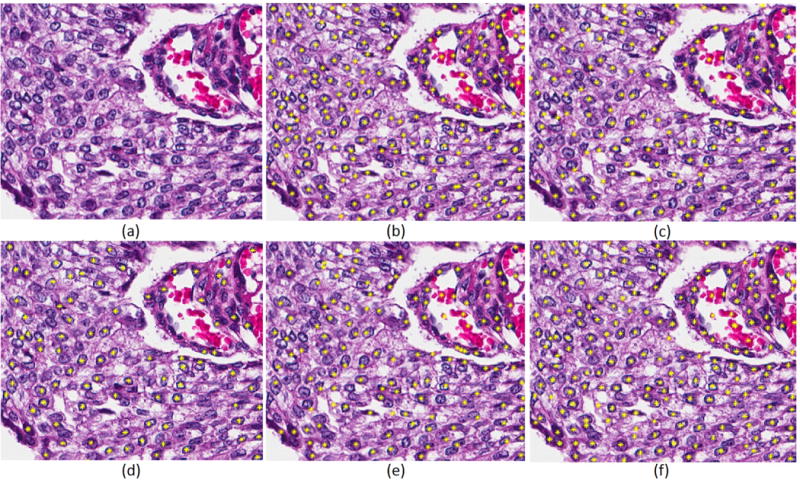
Detected nuclei are highlighted by yellow stars. (a) Original image, (b) NMF(LoG)+ShCNN, (c) BR+ShCNN, (d) LoG of the blue channel, (e) LoG of BR+ShCNN, and (d) LoG of NMF(LoG)+ShCNN (proposed).

Our annotated image database consists of nuclei with many phenotypes which can be due to either aberrant nuclear architecture or poor staining. For example, a subset of nuclei have a vesicular phenotype. Therefore, to improve the detection profile, two separate networks with the same architecture, are trained with vesicular and non-vesicular samples. The results of these two networks are then fused. Two policies for fusion were examined: (i) “addition” of the probability maps of the two networks, as shown in Figure 5, and (ii) replacing the “addition” operator by training a third CNN. The latter approach did not produce superior results, but the first policy improved the F-Score, precision, and recall of LoG of NMF(LoG)+ShCNN to 0.8707, 0.9036 and 0.8401. Overall, fusion improved the results by around 3%.

Fig. 5.

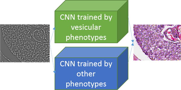
Two separate CNNs are trained by different phenotypes (e.g., vesicular), and computed probability maps are added for nuclei detection.

The above experiments have been implemented by random patch selection of section III with a dataset of 200,000 sample patches. It should be noted that random selection enables an almost infinite number of patch generation; hence, no data augmentation is needed. Alternatively, one can select nuclei centered patches with data augmentation. With equal training and testing datasets between these two policies, nuclei-centered patches result in an inferior performance of 0.6256, 0.6378, and 0.6139 for F-Score, precision, and recall, respectively.

Figure 6 shows the performance of the nuclear detection using LoG of NMF(LoG) on a diverse set of nuclear phenotypes from brain and breast tumors. In the case of brain tumors, the phenotype includes normal and malignant, viable tumors mixed with infiltration of lymphocytes, and vesicular nuclei. In the case of breast cancer, nuclei are detected in the context of collagen scaffolding and mammary glands. The goal is to demonstrate strength and weaknesses of the current method for nuclear detection.

Fig. 6.

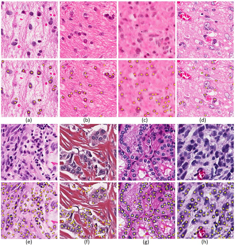
Qualitative performance representation for detection of nuclei (a) with normal organization in GBM; (b–c) having imaging artifacts; (d) having either vesicular or potentially necrotic phenotypes; (e) with viable GBM and infiltrating lymphocytes, (f–g) in the context of collagen and mammary gland architecture; and (h) with proliferating and pleomorphic tumor cells.

C. Sensitivity Analysis for the Shallow CNN

The input patch size of the shallow CNN was modulated from 31 to 71 to determine the optimum detection performance empirically. In all cases, CNN was trained with the LoG of NMF(LoG) representation. The results, shown in Table V, indicate that the performance increases as a function of the patch size, levels off between 41 and 51, and then decreases. Thus, the selection of patch size of 51-by-51 is empirically justified. A possible explanation is that the patch sizes of 41-by-41 to 51-by-51 cover a range which is the double the size of nuclear variations.

TABLE V.

Performance evaluation as a function of the patch size

Input size	Recall	Precision	F-Score	Over-detected
31 × 31	0.7120	0.6970	0.7039	0.0965
41 × 41	0.9170	0.7763	0.8408	0.0880
51 × 51	0.8104	0.8820	0.8447	0.0600
61 × 61	0.8552	0.7916	0.8222	0.0816
71 × 71	0.6192	0.8420	0.6645	0.0716

D. Over-fitting Analysis

For the Deep CNN, the dropout technique has been used to avoid over-fitting. For the Shallow CNN, the learning curve was monitored by measuring the classification accuracy on the training and testing data. The results, shown in Figure 7, indicate that over-fitting did not happen since there is no abrupt decrease in the testing accuracy. In addition, the classification accuracies of the training and testing data as a function of increased number of training samples are shown in Figure 8.

Fig. 7.

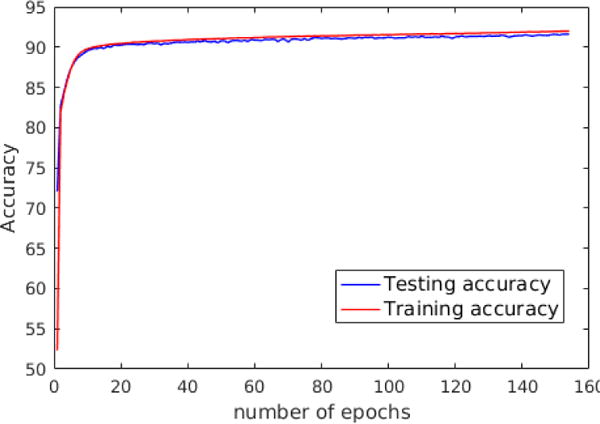
There is no abrupt decrease in the testing accuracy; therefore, over-fitting does not happen.

Fig. 8.

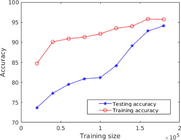
The difference of classification accuracies is decreased between the training and testing data as a function of increased number of training samples.

E. Detection of 3D Nuclei in samples imaged with confocal microscopy

Colony formation is an important facet for profiling of 3D multicellular systems, and the first step is to detect nuclei. Once nuclei are detected, important colony indices (e.g., flatness, size, elongation) can be computed [10], [31]. Detection of 3D nuclei representation is evaluated with the same configuration of the network architecture for 2D detection. However, in this case, there is no need for color decomposition. The detection of nuclei has been validated with four human mammary epithelial cell (HMEC) lines with diverse genetic diversity. These include (a) premalignant line of MCF10a, (b) ductal carcinoma in situ (DCIS) model of MCF7, (c) EGFR positive model MDA-MB-468, and (d) triple negative model of MDA-MB-231. Such a strategy has an added value that validation is not cell-line specific. The nomenclatures of this section are as follows:

• LoG+ShCNN: LoG of raw data with the shallow convolutional neural network.

• Raw+ShCNN: Raw input with the Shallow convolutional neural network.

• IV: Iterative voting[14].

Table VI shows the performance of 3D nuclear detection using shallow CNN, where the performance is also compared with the 3D implementation of iterative voting technique [32], [14]. The significance of this experiment is that CNN, with automatically learned kernels, performs slightly better than carefully crafted algorithm such as iterative voting. It is also important to note that the DCNN design did not improve nuclear detection profile, which was the same case for detecting nuclei from 2D images. Finally, detection of nuclei is shown in two different panels. In Figure 9, nuclear detection results are overlaid on a single focal plane of the 3D image stack. In Figure 10, nuclei are detected and represented as 3D spots, organization of spots are represented with Delaunay triangulation, and organizations are visualized by their outer surfaces as well as triangulated edges. These results clearly show that the premalignant line of MCF10a and DCIS line of MCF7 organize as spheroids; however, the other two lines are more flat and elongated–an observation that is consistent with published literature [10].

TABLE VI.

Nuclei detection results of 3D Data

Method	Recall	Precision	F-Score	Over-detected
LoG+ShCNN	0.8534	0.9394	0.8944	0.0337
Raw+ShCNN	0.8228	0.8908	0.8555	0.1225
Iterative Voting[14]	0.8600	0.8700	0.8649	unkhown

Fig. 9.

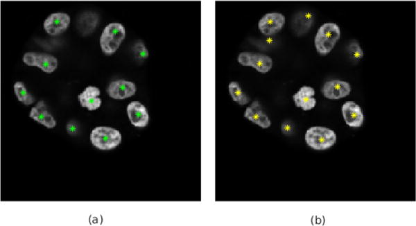
Detected nuclei of 3D fluorescent images in 2D from. (a) and (b) show the results of using the raw image and LoG of gray image as CNN inputs, respectively.

Fig. 10.

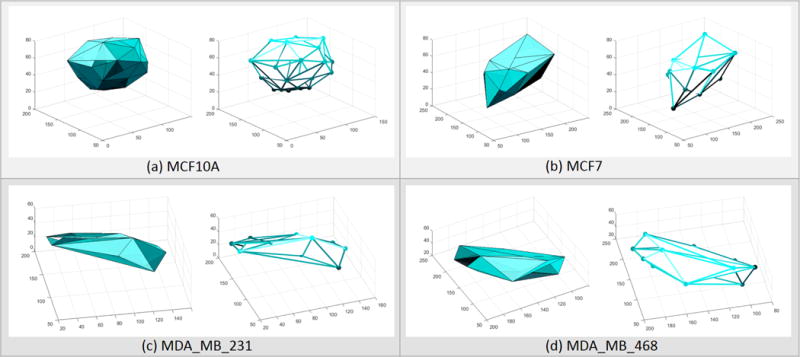
Detection of nuclei contributes to colony profiling in multicellular assays. Colony formation of one premalignant cell line and three breast cancer cell lines are shown in (a), (b), (c), (d)

V. Conclusion

Experiments in this paper indicate that robust initialization of the NMF, with the statistics collected by the LoG response of the image, improves color decomposition when compared to prior methods. In addition, nuclear detection with CNN is improved (a) by color decomposition, and (b) the LoG response corresponding to the computed nuclear channel following CD. The LoG filter accentuates underlying spatial distribution of the nuclei regions and performs a rudimentary initial detection. These observations suggest that accurate color decomposition and application of engineered features to the image are important for improved nuclear detection. Furthermore, one of the major challenges for nuclear detection has been the vesicular phenotypes, which can be biologically relevant or be the result of poor sample preparation. However, the proposed fusion model has improved the detection rate for this class of phenotype. The same framework, but with the exclusion of the color decomposition, has been applied to 3D multicellular systems that have been imaged with confocal microscopy. The results indicate improved performance without any complex algorithmic development. In addition, multiple training strategies have revealed that random patch selection, as opposed to nuclei-centered patch selection, provides a better training model. A plausible explanation is that random selection (i) offers increased diversity, and (ii) contains information about the cellular organization (e.g., adjacent nuclei). In contrast, the required data augmentation (e.g., affine transformation, elastic deformation) for nuclei centered-patches does not generate sufficient diversity. Finally, in a very small number of cases, some nuclei with visually sharp contrast are missed. Further analysis of the corresponding probability maps indicated unusually low probabilities for these nuclei. Since this phenomenon usually occurs for fibroblasts and that these cell types were rarely included in the training set, our conjecture is that deep learning integrates coupled representation of shape and intensity for detection of nuclei. This is an interesting observation since it allows the detection of nuclei to be limited to tumor and epithelial cells while the stromal cells (e.g., fibroblast) are excluded from higher level analysis. Future research may include increasing the diversity of the LoG response filters with the difference of oriented Gaussian filters. These filters have the advantage of preferred orientation for accentuating elongated nuclei (e.g., fibroblast, mesenchymal cells).

References

- 1.Rajan R, Poniecka A, Smith TL, Yang Y, Frye D, Pusztai L, Fiterman DJ, Gal-Gombos E, Whitman G, Rouzier R, Green M, Kuerer H, Buzdar AU, Hortobagyi GN, Symmans WF. Change in tumor cellularity of breast carcinoma after neoadjuvant chemotherapy as a variable in the pathologic assessment of response. Cancer. 2004;100(7):1365–1373. doi: 10.1002/cncr.20134. [Online]. Available: http://dx.doi.org/10.1002/cncr.20134. [DOI] [PubMed] [Google Scholar]
- 2.Veta M, Pluim JPW, van Diest PJ, Viergever MA. Breast cancer histopathology image analysis: A review. IEEE Transactions on Biomedical Engineering. 2014 May;61(5):1400–1411. doi: 10.1109/TBME.2014.2303852. [Online]. Available: http://dx.doi.org/10.1109/TBME.2014.2303852. [DOI] [PubMed] [Google Scholar]
- 3.Lawrence EM, Warren AY, Priest AN, Barrett T, Goldman DA, Gill AB, Gnanapragasam VJ, Sala E, Gallagher FA. Evaluating prostate cancer using fractional tissue composition of radical prostatectomy specimens and pre-operative diffusional kurtosis magnetic resonance imaging. PLOS ONE. 2016 Jul;11(7):1–12. doi: 10.1371/journal.pone.0159652. [Online]. Available: http://dx.doi.org/10.1371%2Fjournal.pone.0159652. [DOI] [PMC free article] [PubMed] [Google Scholar]
- 4.Chang H, Han J, Borowsky A, Loss L, Gray JW, Spellman PT, Parvin B. Invariant delineation of nuclear architecture in glioblastoma multiforme for clinical and molecular association. IEEE Transactions on Medical Imaging. 2013 Apr;32(4):670–682. doi: 10.1109/TMI.2012.2231420. [Online]. Available: http://dx.doi.org/10.1109/TMI.2012.2231420. [DOI] [PMC free article] [PubMed] [Google Scholar]
- 5.Kothari S, Phan JH, Moffitt RA, Stokes TH, Hassberger SE, Chaudry Q, Young AN, Wang MD. Automatic batch-invariant color segmentation of histological cancer images. 2011 IEEE International Symposium on Biomedical Imaging: From Nano to Macro. 2011 Mar;:657–660. doi: 10.1109/ISBI.2011.5872492. [Online]. Available: http://dx.doi.org/10.1109/ISBI.2011.5872492. [DOI] [PMC free article] [PubMed]
- 6.Kothari S, Phan JH, Osunkoya AO, Wang MD. Proceedings of the ACM Conference on Bioinformatics, Computational Biology and Biomedicine, ser BCB ’12. New York, NY, USA: ACM; 2012. Biological interpretation of morphological patterns in histopathological whole-slide images; pp. 218–225. [Online]. Available: http://doi.acm.org/10.1145/2382936.2382964. [DOI] [PMC free article] [PubMed] [Google Scholar]
- 7.Latson L, Latson L, Sebek B, Sebek B, Powell KA, Powell KA. Automated cell nuclear segmentation in color images of hematoxylin and eosin-stained breast biopsy. Analytical and quantitative cytology and histology / the International Academy of Cytology [and] American Society of Cytology. 2003 Dec;25(6):321–331. [Online]. Available: http://view.ncbi.nlm.nih.gov/pubmed/14714298. [PubMed] [Google Scholar]
- 8.Al-Kofahi Y, Lassoued W, Lee W, Roysam B. Improved automatic detection and segmentation of cell nuclei in histopathology images. IEEE Transactions on Biomedical Engineering. 2010 Apr;57(4):841–852. doi: 10.1109/TBME.2009.2035102. [Online]. Available: http://dx.doi.org/10.1109/TBME.2009.2035102. [DOI] [PubMed] [Google Scholar]
- 9.Bilgin CC, Kim S, Leung E, Chang H, Parvin B. Integrated profiling of three dimensional cell culture models and 3d microscopy. Bioinformatics. 2013;29:3087–3093. doi: 10.1093/bioinformatics/btt535. [Online]. Available: http://dx.doi.org/10.1093/bioinformatics/btt535. [DOI] [PMC free article] [PubMed] [Google Scholar]
- 10.Bilgin CC, Fontenay G, Cheng Q, Chang H, Han J, Parvin B. Biosig3d: High content screening of three-dimensional cell culture models. PLOS ONE. 2016 Mar;11(3):1–19. doi: 10.1371/journal.pone.0148379. [Online]. Available: http://dx.doi.org/10.1371%2Fjournal.pone.0148379. [DOI] [PMC free article] [PubMed] [Google Scholar]
- 11.Xing F, Yang L. Robust nucleus/cell detection and segmentation in digital pathology and microscopy images: A comprehensive review. IEEE Reviews in Biomedical Engineering. 2016;9:234–263. doi: 10.1109/RBME.2016.2515127. [Online]. Available: http://dx.doi.org/10.1109/RBME.2016.2515127. [DOI] [PMC free article] [PubMed] [Google Scholar]
- 12.Adiga U, Malladi R, Fernandez-Gonzalez R, de Solorzano CO. High-throughput analysis of multispectral images of breast cancer tissue. IEEE Transactions on Image Processing. 2006 Aug;15(8):2259–2268. doi: 10.1109/tip.2006.875205. [Online]. Available: http://dx.doi.org/10.1109/TIP.2006.875205. [DOI] [PubMed] [Google Scholar]
- 13.Park C, Huang JZ, Ji JX, Ding Y. Segmentation, inference and classification of partially overlapping nanoparticles. IEEE Transactions on Pattern Analysis and Machine Intelligence. 2013 Mar;35(3):1–1. doi: 10.1109/TPAMI.2012.163. [Online]. Available: http://dx.doi.org/10.1109/TPAMI.2012.163. [DOI] [PubMed] [Google Scholar]
- 14.Parvin B, Yang Q, Han J, Chang H, Rydberg B, Barcellos-Hoff MH. Iterative voting for inference of structural saliency and characterization of subcellular events. IEEE Trans Image Processing. 2007;16:615–623. doi: 10.1109/tip.2007.891154. [Online]. Available: http://dx.doi.org/10.1109/TIP.2007.891154. [DOI] [PubMed] [Google Scholar]
- 15.Veta M, van Diest PJ, Kornegoor R, Huisman A, Viergever MA, Pluim JPW. Automatic nuclei segmentation in h&e stained breast cancer histopathology images. PLOS ONE. 2013 Jul;8(7) doi: 10.1371/journal.pone.0070221. [Online]. Available: http://dx.doi.org/10.1371%2Fjournal.pone.0070221. [DOI] [PMC free article] [PubMed] [Google Scholar]
- 16.Loy G, Zelinsky A. Fast radial symmetry for detecting points of interest. IEEE Transactions on Pattern Analysis and Machine Intelligence. 2003 Aug;25(8):959–973. [Online]. Available: http://dx.doi.org/10.1109/TPAMI.2003.1217601. [Google Scholar]
- 17.LeCun Y, Bengio Y, Hinton GE. Deep learning. Nature. 2015;521(7553):436–444. doi: 10.1038/nature14539. [Online]. Available: http://dx.doi.org/10.1038/nature14539. [DOI] [PubMed] [Google Scholar]
- 18.Xie Y, Xing XKF, Liu F, Su H, Yang L. Medical Image Computing and Computer-Assisted Intervention-MICCAI. New York: Springer; 2015. Deep voting: A robust approach toward nucleus localization in microscopy images; pp. 374–382. [DOI] [PMC free article] [PubMed] [Google Scholar]
- 19.Sirinukunwattana K, Raza SEA, Tsang YW, Snead DRJ, Cree IA, Rajpoot NM. Locality sensitive deep learning for detection and classification of nuclei in routine colon cancer histology images. IEEE Transactions on Medical Imaging. 2016 May;35(5):1196–1206. doi: 10.1109/TMI.2016.2525803. [Online]. Available: http://dx.doi.org/10.1109/TMI.2016.2525803. [DOI] [PubMed] [Google Scholar]
- 20.Lee DD, Seung HS. In NIPS. MIT Press; 2000. Algorithms for non-negative matrix factorization; pp. 556–562. [Google Scholar]
- 21.Lee D, Seung H. Learning the parts of objects by nonnegative matrix factorization. Nature. 1999;401:788–791. doi: 10.1038/44565. [DOI] [PubMed] [Google Scholar]
- 22.Ingle J, Crouch S. Spectrochemical Analysis. NJ: Englewood Cliffs; 1988. [Google Scholar]
- 23.Simonyan K, Zisserman A. Very deep convolutional networks for large-scale image recognition. CoRR. 2014;abs/1409.1556 [Online]. Available: http://arxiv.org/abs/1409.1556. [Google Scholar]
- 24.Srivastava N, Hinton G, Krizhevsky A, Sutskever I, Salakhutdinov R. Dropout: A simple way to prevent neural networks from overfitting. J Mach Learn Res. 2014 Jan;15(1):1929–1958. [Online]. Available: http://dl.acm.org/citation.cfm?id=2627435.2670313. [Google Scholar]
- 25.Khan AM, Rajpoot N, Treanor D, Magee D. A nonlinear mapping approach to stain normalization in digital histopathology images using image-specific color deconvolution. IEEE Transactions on Biomedical Engineering. 2014 Jun;61(6):1729–1738. doi: 10.1109/TBME.2014.2303294. [Online]. Available: http://dx.doi.org/10.1109/TBME.2014.2303294. [DOI] [PubMed] [Google Scholar]
- 26.Macenko M, Niethammer M, Marron JS, Borland D, Woosley JT, Guan X, Schmitt C, Thomas NE. A method for normalizing histology slides for quantitative analysis. 2009 IEEE International Symposium on Biomedical Imaging: From Nano to Macro, June. 2009:1107–1110. [Online]. Available: http://dx.doi.org/10.1109/ISBI.2009.5193250.
- 27.Rabinovich A, Agarwal S, Laris C, Price JH, Belongie SJ. Unsupervised color decomposition of histologically stained tissue samples. In: Thrun S, Saul LK, Schölkopf PB, editors. Advances in Neural Information Processing Systems 16. MIT Press; 2004. pp. 667–674. [Online]. Available: http://papers.nips.cc/paper/2497-unsupervised-color-decomposition-of-histologically-stained-tissue-samples.pdf. [Google Scholar]
- 28.Ruifrok A, Johnston D. Quantification of histochemical staining by color deconvolution. Anal and Quant Cytol Histol. 2001 Aug;5:291–299. [PubMed] [Google Scholar]
- 29.Rajpoot N. Stain normalization toolbox. 2015 Jan; [Online]. Available: http://www.warwick.ac.uk/fac/sci/dcs/research/combi/research/bic/software/sntoolbox/
- 30.Glorot X, Bengio Y. Understanding the difficulty of training deep feedforward neural networks. JMLR W&CP: Proceedings of the Thirteenth International Conference on Artificial Intelligence and Statistics (AISTATS 2010) 2010 May;9:249–256. [Google Scholar]
- 31.Cheng Q, Bilgin CC, Fonteney G, Chang H, Henderson M, Han J, Parvin B. Stiffness of the microenvironment upregulates erbb2 expression in 3d cultures of mcf10a within the range of mammographic density. Sci Rep. 2016;6:28987. doi: 10.1038/srep28987. 2016 [Online]. Available: http://dx.doi.org/10.1038/srep28987. [DOI] [PMC free article] [PubMed] [Google Scholar]
- 32.Han J, Chang H, Yang Q, Fontenay G, Groesser T, Barcellos-Hoff MH, Parvin B. Multiscale iterative voting for differential analysis of stress response for 2d and 3d cell culture models. J Microsc. 2011 Mar;241:315–26. doi: 10.1111/j.1365-2818.2010.03442.x. 2011. [DOI] [PubMed] [Google Scholar]