

Abstract
This paper proposes a bio-inspired visual motion estimation algorithm based on motion energy, along with its compact very-large-scale integration (VLSI) architecture using low-cost embedded systems. The algorithm mimics motion perception functions of retina, V1, and MT neurons in a primate visual system. It involves operations of ternary edge extraction, spatiotemporal filtering, motion energy extraction, and velocity integration. Moreover, we propose the concept of confidence map to indicate the reliability of estimation results on each probing location. Our algorithm involves only additions and multiplications during runtime, which is suitable for low-cost hardware implementation. The proposed VLSI architecture employs multiple (frame, pixel, and operation) levels of pipeline and massively parallel processing arrays to boost the system performance. The array unit circuits are optimized to minimize hardware resource consumption. We have prototyped the proposed architecture on a low-cost field-programmable gate array platform (Zynq 7020) running at 53-MHz clock frequency. It achieved 30-frame/s real-time performance for velocity estimation on 160 × 120 probing locations. A comprehensive evaluation experiment showed that the estimated velocity by our prototype has relatively small errors (average endpoint error < 0.5 pixel and angular error < 10°) for most motion cases.
Index Terms: Bio-inspired motion estimation, motion energy, multiple levels of pipeline, optical flow, spatiotemporal filtering, very-large-scale integration (VLSI) architecture
I. Introduction
Real-time visual motion velocity estimation serves as the foundation of many computer vision applications such as object tracking [1], collision prediction [2], [3], depth extraction [4], scene analysis [5], action recognition [6], video compression [7], and retrieval [8], as well as some important biomedical applications [9], [10]. A variety of algorithms have been proposed for motion estimation, including block matching [11], Horn–Schunck method [12], Lucas–Kanade method [13], and phase-based method [14], [15], among others. Most of these methods are essentially based on the spatial coherence of pixel or local patch brightness and contrast during motion [16]–[19]. Recently, bio-inspired algorithms based on motion energy model [20]–[22] have gained an increasing attention. The motion energy-based algorithms are inspired by the motion perception mechanism in primate visual system. These algorithms provide good robustness against noise [20] and easy portability to other bio-inspired visual processing modalities, such as collision estimation, in an integrated framework [23]. The motion energy concept was first introduced in [20]. From then on, many computational motion energy models have been proposed from visual system modeling perspective [20], [24]–[27]. They commonly divide the motion estimation task into two stages, roughly corresponding to V1 and MT neurons in primate visual cortex. The first stage filters the image sequence with a set of spatiotemporal filters tuned to different spatiotemporal frequencies. The results on each probing location are regarded as a motion energy distribution in spatiotemporal frequency space for that location. The second stage then integrates the motion energy distribution into velocity information for each probing location. These existing models differ from each other mostly by how they compute the motion energy distribution and integrate such distribution into velocity. Moreover, the model proposed in [28] adds a retina-like stage before spatiotemporal filtering. It enables the original 2D velocity estimation to be decomposed into independent estimations of two orthogonal 1D velocity components, thereby significantly reducing computational overhead.
At the same time, various software and very-large-scale integration (VLSI) hardware prototypes based on those motion energy models have been implemented [23]–[34]. In [23], a software approach utilized the estimated velocities to evaluate time to collision for obstacle avoidance. To achieve real-time performance, 14 general-purpose computers were employed with 100-Mb/s Ethernet links. Its huge system volume and cost forbid it to be employed in real applications. Another software implementation computed motion energy features and directly used them to track pedestrians without explicit velocity integration [29]. The implementation achieved 25 frames/s as the application required only motion energy computation in small tracked regions. A similar work was done in [30], yet without any information on its real-time performance. On the other hand, some VLSI implementations based on analog application-specific chips were proposed [28], [31]–[33]. In these systems, multiple chips were required to compute the motion energy, and a general-purpose computer was used for velocity integration. Their high system cost and power consumption are not suitable for embedded applications. Recently, a few digital VLSI prototypes based on field-programmable gate array (FPGA) platforms have been proposed [34], [35]. They provide lower cost, higher precision, and higher flexibility compared with software implementations and analog chips. In [34], the extracted motion energy features are only for object tracking without explicit velocity integration, the same as the implementations in [29] and [30]. The other one in [35] partially improves the model in [28]. However, it still involves complicated operations such as division, and consumes most resource of Xilinx Virtex-6 on ML605 evaluation board.
In this paper, we have the following contributions in developing bio-inspired motion estimation for low-cost embedded system.
At the model/algorithm level, we first elaborate the principle of motion energy-based motion estimation, in a more concise and intuitive way than previous literatures. Then we propose a hardware-friendly motion estimation algorithm based on motion energy. Our algorithm combines two important ideas from previous works: decomposing the 2D velocity estimation into two 1D velocity components in [28] and [35] and integrating the motion energy distribution into final velocity by weighted voting [24]. In addition, our contribution also includes an enhancing method mimicking ON and OFF ganglion cells on primate retina, a simple form of velocity voting weights for 1D velocity integration, as well as a confidence map to indicate the reliability of estimation results.
At the hardware level, we propose a compact digital VLSI architecture to run our algorithm. To accelerate processing speed to achieve real-time performance, we employ multiple levels (frame, pixel, and operation levels) of pipeline, as well as massively parallel processing arrays. To reduce hardware resource consumption, the circuit structures of those array units are carefully designed and optimized. In particular, we reduce the amount of multipliers from 492 to 147 without any change to our original algorithm. A prototype of our VLSI architecture is implemented on a low-cost FPGA platform (Zedboard Zynq-7020), achieving 30-frame/s velocity estimation on a 160 × 120 grid of probing locations.
We conducted comprehensive evaluation experiments using benchmark images from real world to show that the performance of our hardware system is comparable with many other visual motion (optical flow) estimation algorithms running on PC or on various hardware platforms, including the well-known Lucas–Kanade method. The rest of this paper proceeds as follows. In Section II, we propose our bio-inspired motion estimation algorithm. The compact digital VLSI architecture with its pipeline schemes and parallel array circuit structures is presented in Section III. In Section IV, an FPGA prototype of our VLSI architecture is implemented and evaluated. We will discuss some issues with the proposed system, and compare our work with previous work in this section. Finally, Section V concludes this paper.
II. Motion Estimation Algorithm
A. Algorithm Principle
In primate visual systems, the motion velocity is derived from spatiotemporal responses [36]. This principle is employed in the proposed algorithm. To understand the concept, consider a spatial sine wave with spatial frequency (Ωx, Ωy) moving at a velocity (vx, vy) on 2D image plane (x, y)
| (1a) |
where A and φ represent the amplitude and initial phase of the sine wave, respectively. The signal I for a given location (x0, y0) on the image plane is given by
| (1b) |
This can be regarded as a temporal sine wave at that location, with a temporal frequency Ωt = −Ωx vx − Ωyvy, or
| (1c) |
Apparently, two variables vx and vy cannot be solved given a single set of spatial and temporal frequencies. In reality, motion image sequences usually contain multiple spatiotemporal frequency components (Ωxi, Ωyi, Ωti), i = 1, 2, …, n, around the location (x0, y0). Those components can be extracted and represented by a phase-invariant format called motion energy [22]. For a given velocity (vx, vy) at one location, (1c) indicates that all motion energies should lie exactly on the plane orthogonal to the vector (vx, vy, 1) in the Ωx –Ωy–Ωt space of that location. But due to image discretization in space–time and other noises, the motion energy is usually distributed around that plane, as shown in Fig. 1(a). Thus, velocity estimation can be regarded as fitting such distribution into an optimal (vx, vy, 1) plane. The fitting computation is called velocity integration in this paper.
Fig. 1.

Motion energy distribution. (a) Motion energy distribution in the 3D Ωx –Ωy –Ωt space (the motion energy balls shown in green are sparsely drawn for visual clarity, with ball size signifying the energy value). (b) Intersection lines of (vx, vy, 1) plane with Ωx –Ωt and Ωy–Ωt planes. (c) Subsets of motion energy distribution on 2D Ωx –Ωt and Ωy–Ωt planes.
In real applications, the motion energy distribution is sampled at discrete spatial and temporal frequency points. Suppose Ns, Ns, and Nt points are needed for Ωx, Ωy, and Ωt, respectively, calculating motion energy distribution in the 3D Ωx –Ωy–Ωt space is computationally intensive with complexity. However, the optimal (vx, vy, 1) plane can be uniquely represented by its intersection lines with the Ωx –Ωt and Ωy–Ωt planes, as shown in Fig. 1(b). Since the two inter-section lines can be independently characterized by vx and vy, respectively, we need to fit only two straight lines to the motion energy distributions on those 2D planes, to solve vx and vy, separately. Thus, the computation complexity is O(2Ns Nt), as shown in Fig. 1(c). Since it always holds that Ns>2, the computational complexity is reduced. The more important reason to decompose 2D motion estimation into two 1D estimations is that much computational resource can be saved for low-cost hardware implementation, as will be illustrated in Section III-D.
The whole flow of our proposed bio-inspired motion estimation algorithm is shown in Fig. 2, with different processing stages corresponding to different stages in primate visual system. The algorithm details will be disclosed in the following sections, followed by discussion on the correspondence between these stages and their counterparts in primate visual systems.
Fig. 2.

Proposed bio-inspired motion estimation algorithm flow.
B. Preprocessing
This stage includes image rescaling and spatiotemporal frequency extension, by means of antialiasing subsample operation and edge extraction. The 2:1 antialiasing subsample operation is optional and can be cascaded. It aims to rescale the original image to a manageable size, thus providing tradeoff between estimation density (i.e., the number of probing locations for velocity estimation) and processing performance. For low-cost embedded systems, we choose a sampling grid of 160 × 120. Each subsample step uses the same Gaussian filter to remove higher spatial frequencies, and then picks out corresponding pixels to form a 2:1 subsampled image. Next, a Laplacian of Gaussian (LoG) filter followed by ternarization operation with thresholds ±THt transforms the original image to an edge image quantized into three levels of intensity (i.e., 1, 0, and −1). Effectively, this processing extends the spatiotemporal frequency band to ensure sufficient motion energy distributed on the Ωx –Ωt and Ωy–Ωt planes. The ternarization operation mimics retina ON–OFF cells and cancels out spatial dc components (i.e., Ωx = Ωy = 0) that may cause ambiguous results on static regions (i.e., Ωt = 0), according to (1c). As the Gaussian and LoG filters are used for their qualitative functions, their specific coefficients need not be quantitatively precise. Therefore, we choose the coefficients to be powers of two for ease of hardware computation, as shown in Fig. 2.
C. Spatiotemporal Filtering
This stage computes the motion energy distribution on the Ωx –Ωt and Ωy–Ωt planes by spatiotemporally filtering the ternary edge image. Although the filters are common Gabor filters as popularly used in many other works and the motion energy is computed in the way proposed in [20], we still exhibit their details in our work for self-containing. Based on these details, we further explore the filter symmetry to reduce computational overhead. Here we explain only the computation on the Ωx –Ωt plane, as on the Ωy–Ωt plane, it is similar. Suppose we expect to sample motion energy units on the Ωx –Ωt plane at these spatiotemporal frequencies: (Ωxi, Ωt j), i = 1, 2, …, m, j = 1, 2, …, n. The first step is temporal filtering, where one temporal frequency Ωt j corresponds to two 1D Gabor filters with orthogonal phases
| (2a) |
| (2b) |
where is a normalized 1-D temporal Gaussian kernel centered at t = 0, with a standard deviation of and an extension of Et frames (i.e., the filter length is 2Et + 1). However, for real-time causality, the filter has to be delayed by Et frames when all required sequence frames are ready. In other words, we have to convolve the image sequence with Gae(o)(t − Et, Ωt j) rather than Gae(o)(t, Ωt j). Next, as explained earlier in Section II-A, we need to compute the motion energy distribution on the Ωx –Ωt plane where Ωy = 0. To extract the frequency component with Ωy = 0, a 1D low-pass filtering along the y-axis is needed to perform on the 2n temporally filtered images. To realize such low-pass filtering, we choose a 1D averaging filter with a spatial length of (2Es + 1) pixels along the y-axis. This filter simply sums up all pixel intensities covered by it. After that, each one of those filtered images is passed through another set of 2m 1D spatial Gabor filters along the x-axis. Likewise, one spatial frequency Ωxi corresponds to two filters Gae(o)(x, Ωxi) similar to (2), but with 1D spatial Gaussian kernel along the x-axis. As a result, 2m× 2n spatiotemporally filtered images are produced.
Finally, the phase-invariant motion energy units on each probing location for each spatiotemporal frequency (Ωx, Ωt) are extracted as
| (3) |
where I (·) is the spatiotemporally filtered image intensity on that location. Its subscripts indicate whether its spatial and temporal Gabor filters are even (e) or odd (o) phased. The spatiotemporal coordinates (x, y, t) in ME(·) and I (·) are omitted for clarity. From the symmetry property of 1D Gabor filters, we have
| (4) |
| (5) |
Thus, we need to compute only I (·) for Ωx > 0 and Ωt ≥ 0. This significantly reduces computation overhead. For nonnegative Ωx and Ωt, we have Ωx, Ωt ≤ 0.5 × 2π = π, according to the Nyquist Law. However, our experiment suggests that it is better to further lower the maximum Ωx and Ωt for a larger margin against frequency aliasing. We choose the parameters of Ωx(y), Ωt, Es, and Et as listed in Table I for spatiotemporal filters. The values of Es and Et in Table I are chosen to keep the filter size at an acceptable level while not chopping those filters too much. The parameter configuration will be further discussed in Section IV.
TABLE I.
Parameters Used in Our Algorithm
| Parameter | Value | Description |
|---|---|---|
| Et (frame) | 7 | The temporal extension of 1D temporal Gabor filters |
| Ωt (rad/frame) | 2π × 0.075k, k=0, 1, 2, …, 6 | Used temporal frequencies of 1D temporal Gabor filters |
| Es (pixel*) | 10 | The spatial extension of 1D spatial Gabor filters |
| Ωx(y) (rad/pixel) | 2π × {0.1, 0.15, 0.2} | Used spatial frequencies of 1D spatial Gabor filters |
| vmax (pixel/frame) | 2 | Maximum absolute of allowed 1D velocity component on subsampled image |
| vi (pixel/frame) | ±0.1p, p=0, 1, 2, …, 20 | Sampled velocity points for 1D velocity voting |
The word pixel in this table refers to the pixel in the rescaled (subsampled) image and corresponds one point in the estimation grid of original image.
D. Velocity Integration
In this stage, a 1D velocity voting is performed to integrate the motion energy distribution into velocity information. We propose a simple form of voting weights for 1D velocity integration. Our method works in identical way for both vx and vy. It requires a dense sampling vi, i = 1, 2, …, l, between ±vmax, where ±vmax defines allowed velocity range in our algorithm. For each pixel, its motion energy units with different spatiotemporal frequencies (Ωx(y), Ωt) vote for each vi by different weights
| (6) |
where δ is an empirical parameter, and its optimal value may vary for different configurations of temporal filter set. For simplicity, we set it to 0.2π throughout this paper. The weight reflects the approximate Gaussian distribution of motion energy around the line indicated by vi on the Ωx(y)–Ωt plane, as mentioned in Section II-A. Moreover, as indicated by (5) and (6), ME(−Ωx(y), ±Ωt) and ME(Ωx(y), ŦΩt) have equal votes, so we can use only the motion energy units with Ωx(y) > 0. This converts (6) into a unified format involving only nonnegative parameters (i.e., Ωx(y), |Ωt |, and |vi |) for computation
| (7) |
Finally, a winner-take-all (WTA) operation is performed on each probing location. The vi with maximum voting score from all motion energy units on one location is regarded as its estimated velocity vx(y). Although the sampling interval of vi inevitably introduces some estimation error, it will not dominate overall errors if sampled densely enough, according to our experimental results. Table I lists our velocity samples.
In our algorithm, the spatiotemporal filter coefficients in (2) and velocity voting weights in (7) do not change during runtime. They can be statically determined beforehand. Therefore, the runtime performance will not be affected by the complexity in computing these coefficients and weights.
E. Confidence Map
The estimated velocity in a texture-less region may be inaccurate and unreliable. To tackle this problem, we propose a confidence map that is generated from the local spatiotemporal texture abundance. For each probing location, the absolute pixel intensities within its (2Es + 1) × (2Es + 1) spatial neighborhood over the latest (2Et + 1) ternary image frames are summed up, and then thresholded by THs to generate a flag on corresponding location in the confidence map. The flag determines if the estimated velocity is reliable or not on that location. The usage of the confidence map can assist further processing based on the estimated velocity information, as will be discussed in Section IV.
F. Bio-Inspired Features
The major stages in our algorithm can find their counterparts in primate visual system for motion speed estimation. There are at least three types of neurons that play critical roles in motion perception in the primate visual system: the ON–OFF ganglion cells in the retina, the simple/complex neurons in the primary cortex V1, and MT neurons in higher level cortex. The ON–OFF cells can be excited by image edges and temporal light changes. For spatially and temporally constant stimuli, these ON/OFF cells do not respond. This attribute is crucial for biological visual systems to achieve a wide dynamic range. From information processing point of view, coding changes is more effective [37]. In the primary visual cortex V1, many simple/complex neurons are tuned to different spatial/temporal frequencies. Each V1 neuron gives maximum responses to its particular frequency. The output signals of V1 neurons are regarded to have the motion velocity information coded [38]. The MT neurons finally decode the velocity speed and direction by combining the V1 neuron output signals [38].
In our proposed bio-inspired algorithm and VLSI system as shown in Fig. 2, the LoG filtering followed by ternarization works in a similar way as the ON–OFF ganglion cells in retina. As a result, the ternarization outcome to positive edges and negative edges is equivalent to the responses of ON–OFF cells. Realized by Gaussian-enveloped Gabor kernel corresponding to a particular frequency, each spatial or temporal filter in our algorithm mimics one spatial or temporal frequency tuned V1 neuron in the primary cortex. The outputs of both the biologic visual system and the electronic system are array of responses to frequencies of the visual stimuli. The responses of spatiotemporal filtering represented by motion energies in the electronic system are summed up at the velocity integration stage to generate the final motion estimation. This integration computation realized by velocity voting is essentially the same as how the MT neurons combine the afferent signals from V1 neurons [50]. Fig. 2 shows how afferent signals are summed up.
III. VLSI Architecture
A. System Overview
The block diagram of the proposed digital VLSI architecture for bio-inspired visual motion estimation is shown in Fig. 3. It includes optionally cascaded Gaussian filters with 2:1 sub-sample function, an LoG filter with ternarization function, a velocity estimation block, a sequencer, a parameter register bank, and some memory buffers. The velocity estimation block contains four massively parallel processing arrays, a WTA unit, and a confidence flag generator. When a new image frame arrives, the Gaussian filters produce a rescaled image and store it into the buffer. Then the LoG filter reads the rescaled image and produces a new frame of ternary image to update the ternary image buffer containing the most recent (2Et + 1) frames of ternary images. Then the velocity estimation block estimates pixel velocities from the ternary images. For each probing location, its neighboring pixels in the ternary images are processed by the temporal and spatial Gabor filter arrays. Next, the motion energy units are extracted from the filtered results by motion energy extractor array, and are used in velocity voter array for velocity voting. Finally, the WTA component decides the winning velocity, and stores it along with the confidence flag into the output buffer. The sequencer controls the overall system operations, and the parameter register bank assigns filter coefficients and voting weights. Once vx and vy are estimated, the velocity estimation block moves to the next probing location, and repeats the operations described above.
Fig. 3.

Proposed VLSI hardware architecture for bio-inspired visual motion estimation.
To realize real-time performance, we propose multiple levels of pipeline for the system. This makes full utilization of the parallel arrays and other processing components, as will be discussed in Section III-B. Moreover, all the array units are running in parallel to reduce processing time. Each unit in one array has identical circuit structure and operates under the same control signals, but with different data. The circuit structures of array units are optimized to minimize hardware consumption, as will be revealed in Sections III-C and III-D. The parameter register bank is programmable, so as to allow different filters and voting rules if needed.
B. Multiple Levels of Pipeline
In this architecture, we propose three levels of pipeline as follows to improve the system performance.
1. Frame-Level Pipeline
This pipeline contains three stages and enables our system to handle three image frames concurrently, as shown in Fig. 4(a). At one point of time, the external image sensor is capturing a new frame, and the Gaussian filter is producing subsampled pixels simultaneously in an on-the-fly fashion (i.e., once new pixel data are received from the image sensor that serially sends out pixel data, the Gaussian filter just processes it and produces corresponding result, in a matched rate with the image sensor). At the same time, the velocity estimation block is processing the last frame to compute velocities on each pixel location, while the velocity results of the second last frame are being outputted or under further processing. With such pipeline scheme, the processing time of velocity computation results’ outputs (with optional further processing) are hidden behind the image sensor frame time, as the three tasks can be simultaneously performed for different frames. Therefore, the overall system performance is improved.
Fig. 4.

Multiple levels of pipeline. (a) Frame-level pipeline in whole system. (b) Pixel-level pipeline in velocity estimation block.
2. Pixel-Level Pipeline
To actually realize the above frame-level pipeline, one critical constraint is that the total processing time of LoG filter and velocity estimation block must be less than the image sensor frame period. To reduce the processing time of velocity estimation block, we propose a pixel-level pipeline, as shown in Fig. 4(b). The processing arrays and other components in the block are divided into three stages in the pipeline. Such a pipeline scheme supports processing two pixels for horizontal and vertical directions concurrently. At one point of time, the temporal Gabor filter array is processing the current pixel location to produce temporally filtered results for both horizontal (x) and vertical (y) directions, while the spatial Gabor filter array is operating on the horizontal results in an on-the-fly fashion as mentioned above. At the same time, the velocity voter array is voting for vertical velocity on previous pixel, while the WTA component is deciding horizontal velocity on the previous pixel. The motion energy extractor array works in serial with the spatial Gabor filter array to reduce scheduling complexity. This is feasible as each motion energy extractor involves only a few simple operations [see (3)] and consumes much less processing time compared with that of spatial Gabor filtering.
3. Operation-Level Pipeline
This pipeline scheme exists inside some filters to accelerate the filtering operations. Its implementation will be described with the filter circuit structures in the following section.
C. Circuit Design
Fig. 5 shows the circuit structure of the Gaussian filter. It employs a snake buffer of registers to realize on-the-fly filtering [34]. We propose a two-stage operation-level pipeline to speed up the Gaussian filtering. The 2:1 subsample is achieved via lowest bits of row and column indices. As all filter coefficients are integer powers of two (Fig. 2), we use logic-free (only with wire connections) bit shifters rather than expensive multipliers to implement required multiplication operations, as demonstrated in Fig. 5. This further improves processing speed and saves hardware resource. The LoG filter has a similar circuit structure with a larger snake buffer and logic-free bit shifters for multiplication (×12 is decomposed into ×4 and ×8). Its difference from the Gaussian filter is that it has no subsample, and appends a comparator stage for ternarization to its operation-level pipeline.
Fig. 5.

Circuit structure of Gaussian filter with 2:1 subsample function.
Fig. 6 shows the circuit structure of temporal Gabor filter array unit. It contains (2Es + 1) × (2Es + 1) patch buffer registers, a horizontal bank of (2Es + 1) registers, a vertical bank of (2Es + 1) registers, and a kernel filter. The kernel filter carries out the temporal filtering and employs a two-stage operation-level pipeline to improve filtering speed. Based on ternary data characteristics, we propose a pseudomultiplier that is essentially a simple multiplexer for the required multiplication operations, as shown in Fig. 6. Thus, a lot of hardware resource on building true multipliers is saved.
Fig. 6.

Circuit structures of temporal Gabor filter unit.
The Gabor filter array unit works in a column-by-column fashion as follows. The patch buffer holds temporally filtered results of pixels within of a spatial neighborhood of a fixed size (2Es +1) × (2Es +1). We denote the center position of the current neighborhood by (x*, y*). Each horizontal and vertical bank register holds data sum of corresponding patch buffer column and row (i.e., 1D averaging filtered results as explained in Section II-C) for later spatial Gabor filtering, as shown in Fig. 7(a). Then the center of the spatial neighborhood moves to the next column (x*+1, y*). Thus, the register data in patch buffer, horizontal bank, and vertical bank have to be updated to the new neighborhood. To achieve this purpose, first, the horizontal bank is shifted to the left by one register with the bank’s rightmost register data cleared, as the green arrows indicate in Fig. 7(b). Next, the ternary pixels at (xn+1, y0) = (x* + Es + 1, y* − Es) of the latest (2Et + 1) frames, along with filter coefficients, are sent to the kernel filter. The result is shifted into the first patch buffer row, and also accumulated to the rightmost register of the horizontal bank and the vertical bank register in the first row. Meanwhile, the data in the leftmost register in the patch buffer row are subtracted from the vertical bank register in the corresponding row, as indicated by the red arrows in Fig. 7(c). All the operations in Fig. 7(c) are simultaneously performed in one clock cycle. By far, the register data of the first row in the patch buffer and the vertical bank have finished updating. This procedure repeats serially on each of the remaining 2Es rows from top to down, until arriving to the bottom row, as shown in Fig. 7(d) and (e) (the updating from the third row to the second last row is omitted). At this point of time, the data in the rightmost horizontal bank register have also finished its updating. When the unit has finished scanning all the pixels in one row as its center position, it moves on to the next row and the procedure repeats. When the center position is near image border, those patch buffer registers corresponding to pixels outside the image border will be automatically set to zero.
Fig. 7.

Operation flow of temporal Gabor filter unit.
The unit circuit structures of the other three parallel arrays are simply based on multiply accumulator (MAC). In particular, one spatial Gabor filter unit is just a MAC, as shown in Fig. 8(a). It takes (2Es + 1) clock cycles to process the data from the horizontal or vertical bank in one temporal Gabor filter unit. In the motion energy extractor unit in Fig. 8(b), the computations of two motion energy units of symmetrical temporal frequencies (i.e., two frequencies with the same absolute value but opposite signs) share a single MAC in a time-multiplexing fashion. In addition, we employ a short-word multiplier in MAC to complete required long-word multiplication in four clock cycles. Such a multicycle multiplication technique reduces multiplier resource, but increases its processing time from two to eight clock cycles for each pixel. But such an increase will not degrade system performance as it is relatively small to be masked by the processing time of temporal Gabor filtering, due to the pixel-level pipeline scheme as shown in Fig. 4(b). The velocity voter unit in Fig. 8(c) contains two MACs for two voting channels: motion energy of positive temporal frequency corresponds to negative velocity, and vice versa [see (7)]. Again, we use the multicycle multiplication technique to complete one long-word multiplication in two clock cycles. Thus, the unit takes 2×(# of motion energy extractor units) clock cycles to finish voting.
Fig. 8.

Circuit structures of (a) spatial Gabor filter unit, (b) motion energy extractor unit, and (c) velocity voter unit.
Fig. 9 shows the confidence flag generator circuit. Each horizontal bank register holds the sum of absolute pixel data in corresponding spatial neighborhood column over latest ternary frames stored in the ternary buffer. Their total sum is stored in the confidence sum register. The bank works in a similar way to that in the temporal Gabor filter unit. The absolute accumulator computes the sum of absolute values of one pixel over latest ternary frames. It reduces hardware resource because the absolute value of 2-b signed ternary data can be represented only by its lowest bit.
Fig. 9.

Circuit structure of confidence flag generator.
D. Resource Optimization
To realize low-cost hardware implementation, we have employed many resource optimization techniques as described above to reduce the resource consumption, especially to reduce the number of multipliers, because the multiplier is rare resource on FPGA platforms or occupies much more area on an application-specific integrated chip (ASIC). We estimate the reduction in multipliers with our resource optimization techniques in Fig. 10. Suppose we use the same parameters in Table I, with signed 6-b for temporal and spatial Gabor filter coefficients and unsigned 8-b for velocity voting weights. And suppose we use one-stage preprocessing, and one multiplier supports 25 × 18 b (as the case in the prototype FPGA platform used in Section IV-A). If we follow the original model in [24] to directly estimation the 2D velocity vector on the ternary images without any other resource optimization, we would consume as many as 1122 multipliers. By decomposing the 2D velocity estimation into 1D estimations as in our work, the number of multipliers for spatial filters, motion energy extractors, and velocity voters is significantly reduced. The multipliers in the preprocessing Gaussian and LoG filters are removed by the bit-shifting-based multiplication technique as illustrated in Fig. 5. The multipliers for temporal filters are totally removed by our pseudomultiplier technique (see Fig. 6). We further reduce the multipliers in motion energy extractors and velocity voters by the multicycle multiplication technique as mentioned in Section III-C. These four techniques together saved 87% (or 975) multipliers compared with the model in [24], and reduced multipliers from 492 to 147 without compromising our algorithm proposed in Section II.
Fig. 10.

Multiplier resource reduction with optimization techniques.
IV. Implementation and Evaluation
A. Hardware Implementation
To evaluate the performance of our proposed VLSI architecture, an FPGA-based prototype was implemented on the Zedboard Zynq-7020 platform [39] and a testing system was set up, as shown in Fig. 11. The prototype employed one stage of the Gaussian filter with 2:1 subsample in the preprocessing of our algorithm flow. Thus, the prototype allowed estimating velocities on a 160 × 120 grid in one frame for QVGA format (320 × 240) image sensor. Using the parameter configuration in Table I, our prototype contains a 14 × 1 temporal Gabor filter array, a 14 × 6 spatial Gabor filter array, a 21 × 1 motion energy extractor array, and a 21 × 1 velocity voter array in the velocity estimation block. The bit precision is signed 6 b for temporal and spatial Gabor filter coefficients, and unsigned 8 b for velocity voting weights. To simplify the peripheral devices for evaluation, a virtual QVGA image sensor based on on-chip memory has been designed and integrated into the FPGA chip. Video data are dispatched to our motion estimation architecture in a standard sensor timing schedule. The consumed FPGA resources are listed in Table II (excluding the virtual image sensor). Note the total slice consumption is not simply the sum of each module, so we cannot estimate its consumption in other modules in Table II. The FPGA was running at 53-MHz clock frequency, and our architecture achieved 30-frame/s real-time processing performance. We developed a PC software tool to: 1) configure architecture parameters on FPGA prototype; 2) send video image data to FPGA virtual sensor; 3) collect estimated velocity data from FPGA prototype; and 4) display the velocity results labeled upon original video frames. The estimated velocities on the subsampled images on the prototype were scaled back by multiplying a factor of two before it was displayed. The data transfer between the FPGA chip and PC was realized through a high-speed 1000-Mb/s Ethernet link, which was controlled by one of the two hard IP cores of ARM processor integrated in the Zynq-7020 FPGA chip [39].
Fig. 11.
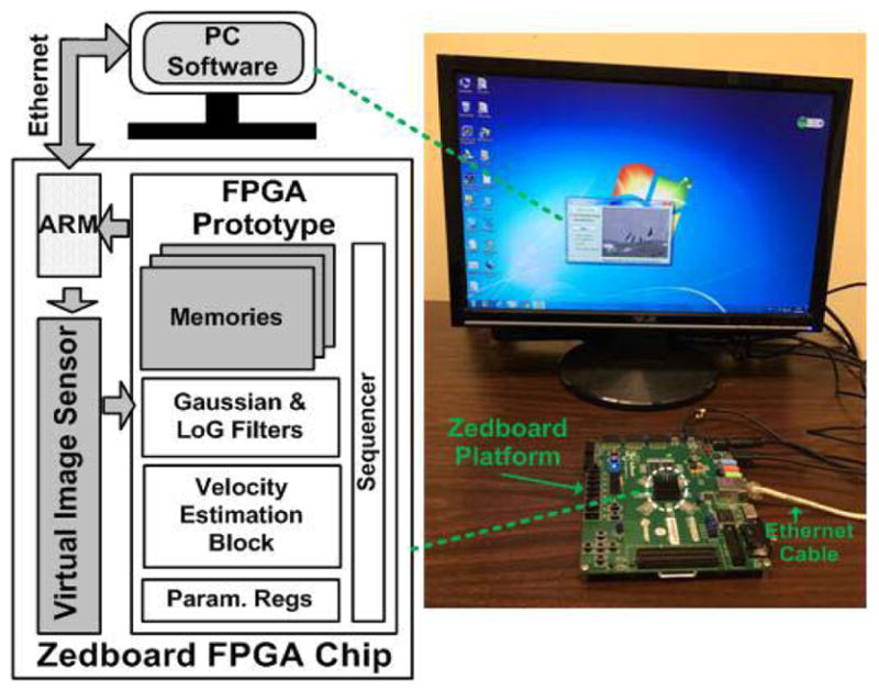
Evaluation system for the FPGA-based prototype of our proposed bio-inspired motion estimation VLSI architecture.
TABLE II.
FPGA Prototype Resource Consumption
| FPGA Resource (Zedboard Zynq-7020) | Slice LUT | Slice Register | Total Slice | Block RAM | DSP (Multiplier/MAC) | BUFGCTRL (Clocking) |
|---|---|---|---|---|---|---|
| Temp. Gabor Filter Array | 20353 | 15862 | 7277 | 0 | 0 | 0 |
| Spatial Gabor Filter Array | 5788 | 2023 | 1736 | 0 | 84 | 0 |
| Motion Energy Extract. Array | 5005 | 4128 | 1596 | 0 | 21 | 0 |
| Velocity Voter Array | 2415 | 4637 | 1070 | 0 | 42 | 0 |
| WTA | 847 | 2724 | 727 | 0 | 0 | 0 |
| Parameter Register Bank | 4965 | 5544 | 2583 | 0 | 0 | 0 |
| Other Modules | 4552 | 570 | - | 31.5 | 0 | 1 |
| Total | 43925/53200 (82.6%) | 35488/106400 (33.4%) | 12597/13300 (94.7%) | 31.5/140 (22.5%) | 147/220 (66.8%) | 1/32 (3.1%) |
B. Qualitative Evaluation
We chose the popular Middlebury benchmark library [40] to evaluate our FPGA prototype. Since no sequence in the library is longer than 2Et + 1 = 15 frames to allow temporal filtering in our system, we generated our own motion sequences using the benchmark images. To generate one sequence, we chose a frame image from the benchmark and resized it to QVGA size. Then the original image was continuously laterally shifted, or rotated, or zoomed in to produce a 15-frame-long motion sequence using a custom MATLAB program. Fig. 12 shows some evaluation results of the three different motion patterns, along with their endpoint error (EE) and angular error (AE) maps. EE and AE calculations are defined in [40]. The displayed velocities with invalid confidence flags (i.e., the flag value is 0) are shown in red dots. The error maps are calculated only on the subsampled 160 × 120 locations in the rescaled image. A ten-pixel wide image boundary on rescaled images was not included in evaluation, and is plotted in red on the error maps along with locations with invalid confidence flags. EE data in range [0, 4] (pixels/frame) and AE data in range [0, 90] (°) are linearly scaled to gray intensity [0, 255] on the maps, while EE > 4 pixels and AE > 90° are set to 255. The error on curtain area for the Rotation sequence is high, due to too much loss of high-frequency spatial features after preprocessing.
Fig. 12.

Velocity estimation results with error maps generated using the proposed approach for some of the benchmark motion sequences. The bigger ends of arrows represent the start points of velocity vectors.
We have also tested the prototype with some real-world sequences we recorded. Fig. 13(a) shows the estimated velocity results on some frames for a driving sequence. Note that some “temporal lags” in Frames 900 and 904 occur to the left of the passing vehicle. This is due to the temporal filtering over 15 frames. While visually the motion vectors do not seem to be on the vehicle, they do represent the average motion of the image region in the past 15 frames. Such latency is inevitable in systems involved with temporal filtering. Its impact on a particular application depends on the frame rate, measures to counter the latency, and the application requirements. Fig. 13(b) shows the estimated velocity results of a walking pedestrian. Note the velocity changes across different regions of his body (e.g., limb and trunk) as well as changes over time. The differences qualitatively demonstrate the spatial and temporal processing resolution of the system.
Fig. 13.

Velocity estimation results on motion sequences in the real world. (a) Driving. (b) Walking.
C. Quantitative Evaluation
To further quantitatively evaluate our algorithm and VLSI architecture, we selected another 12 images from the Middlebury library (see Fig. 14), and again used the custom MATLAB program to generate a series of QVGA-sized 15-frame-long sequences with lateral translation at different speeds (from 0 to 4 pixels/frame at a step of 0.1) and in different directions (0°, 45°, and 90°) to horizontal. For each sequence, we ran it on our FPGA prototype, recorded estimated velocity results and confidence map on the last frame, and computed its average EE and AE of the measured results, over all pixels on the rescaled images except for the ten-pixel-wide boundary and points with invalid confidence flags. Fig. 14 shows the average EE and AE against different motion speeds and directions. In most cases, the errors were small, with average EE < 0.5 pixel and average AE < 10°. The wooden sequences have the highest errors, probably due to the straight edges that are known to easily cause serious aperture problem. Fig. 14 shows that the AE errors are larger for speeds below 0.5 pixel/frame. The reason is that a small error in horizontal or vertical velocity component will cause a relatively significant direction bias for low velocity.
Fig. 14.

Average EE and AE for the benchmark sequences with lateral translation motion. For each of the 12 sequences from Fig. 15, speeds from 0 to 4 pixels/frame in directions 0°, 45°, and 90° were tested.
Fig. 15 shows the average confidence maps for each benchmark image. They are obtained by averaging the confidence maps of sequences with a motion speed of 2 pixels/frame over 12 motion directions (0°, 30°, …, 330°). The values on the maps are scaled to [0, 255] for display. The values within the ten-pixel-wide boundary are manually set to zero. Such average confidence maps can indicate the ability of the proposed algorithm to estimate motion in different image regions. As it can be seen, the system can track most of the image regions for full-field optical flow computation. Only for areas with very low feature density, such as the wall in Basketball and the wooden board in Wooden, or with very high spatial frequency features that may be lost after preprocessing, such as fabric regions in Army and Teddy, the system constantly failed to give motion estimation.
Fig. 15.

Average confidence maps for the 12 benchmark sequences with 2-pixel/frame speed in 12 directions.
For parameter tuning, we compared the average EE and AE under different parameter configurations for spatiotemporal frequencies and velocity voting points, as listed in Table III. The first configuration is the currently used as in Table I. The second to fourth configurations involve different spatial and temporal frequency ranges. The fifth and sixth configurations involve different numbers of temporal and spatial filters. The seventh configuration involves a different set of velocity voting points. All these configurations are under the constraints of hardware resource available on Zynq-7020 chip and real-time processing requirement of 30 frames/s. For the latter three configurations, we slightly adjusted our FPGA prototype for proper processing array sizes in the motion estimation block as shown in Fig. 3. This is easy since our architecture has good scalability. Moreover, to check possible accuracy drop caused by parameter quantization, fixed-point operations, and other hardware simplifications, we ran our algorithm in PC software using parameters and operations in double-precision floating-point format. The Gaussian and LoG filter in the preprocessing also used floating-point coefficients, and their multiplications are carried out directly rather than by bit shifting.
TABLE III.
Different Parameter Configurations
| Conf. | Ωt (rad/frame) | Ωx(y) (rad/pixel) | vi (pixel/frame) |
|---|---|---|---|
| 1 | 2π × 0.075k, k=0, 1, …, 6 | 2π × {0.1, 0.15, 0.2} | ± 0.1p, p=0, 1, …, 20 |
| 2 | 2π × 0.075k, k=0, 1, …, 6 | 2π × {0.05, 0.125, 0.2} | ± 0.1p, p=0, 1, …, 20 |
| 3 | 2π × 0.075k, k=0, 1, …, 6 | 2π × {0.1, 0.175, 0.25} | ± 0.1p, p=0, 1, …, 20 |
| 4 | 2π × 0.05k, k=0, 1, …, 6 | 2π × {0.1, 0.15, 0.2} | ± 0.1p, p=0, 1, …, 20 |
| 5 | 2π × 0.1k, k=0, 1, …, 4 | 2π × {0.1, 0.133, 0.167, 0.2} | ± 0.1p, p=0, 1, …, 20 |
| 6 | 2π × 0.1k, k=0, 1, …, 4 | 2π × {0.05, 0.1,0.15, 0.2} | ± 0.1p, p=0, 1, …, 20 |
| 7 | 2π × 0.075k, k=0, 1, …, 6 | 2π × {0.1, 0.15, 0.2} | ± 0.05p, p=0, 1, …, 40 |
The comparison results are shown in Fig. 16. We tested only with the Dumptruck sequence, because as Fig. 14 shows, the error curves for all sequences except Wooden are very similar. The EE errors of Conf2 and Conf3 are a little higher than Conf1, especially obvious for EE in 0° and 45° and AE in 45°. Curve4 performs better than Curve1 for lower velocity, but its error drastically increases toward higher velocities (>3 pixels/frame horizontal/vertical velocity component). This configuration may be more plausible if we are processing scenes with lower maximum velocity. In contrast, Conf5 and Conf6 (nearly the same in Fig. 16) provide a little lower errors than Conf1 for high velocity, but produces very high errors for low velocity. This demonstrates that the high density of temporal frequencies is more important than that of spatial frequencies, if some tradeoff has to be made under certain constraints. Finally, Conf7 and Conf FL (for floating-point) error curves almost overlap with Conf1 curve. This demonstrates that consuming more hardware resource to sample more velocity voting points barely improves accuracy, and that the parameter quantization, fixed-point operations, and other hardware simplifications do not cause obvious accuracy drop compared with the floating-point software implementation.
Fig. 16.

Average EE and AE for Dumptruck sequence under different parameter configurations (Conf1–7) and software floating-point (Conf FL) version.
Finally, we evaluated the robustness of our system against white Gaussian noise and salt-pepper noise, as shown in Fig. 17. We selected four translation benchmark sequences at a constant horizontal velocity of 2 pixels/frame with different confident region areas of confidence maps in Fig. 14. The noise was independent identically distributed added to each pixel of each sequence frame. The standard deviation of white Gaussian noise was normalized with respect to 255. The results show that our system performs better with Gaussian noise than with salt-pepper noise, as the latter (random white and black dots) more severely interferes the original spatial and temporal frequency components. The results also demonstrate that the texture-less scenes with small confident region (e.g., the Basketball sequence) prune to be affected by noise. The reason is that the noise will trick the system to estimate on otherwise ignored texture-less region, which is now dominated by random noise.
Fig. 17.

System robustness against noise.
D. Comparison With Other Works
Table IV compares our implementation with other bio-inspired motion energy-based motion estimation implementations (second to fourth rows). Relatively, our algorithm and system achieved low complexity, low-cost implementation, and moderate accuracy on challenging motion sequences. The errors in [28] and [35] seem to be lower than ours, but their EE/AE values are evaluated assuming that vertical (y) error is always zero for simplification, which is not always true in real-world cases. Moreover, they consumed high-cost hardware resources, and only evaluated on simple synthesized motion sequences (e.g., white square) rather than cluttered natural or standard benchmark sequences as in our work. The software implementation in [23] cost tremendous resources, but achieved a low frame rate (11 frames/s). They did not provide EE and AE errors since their purpose was to estimate the time to collision, which was of about 20%–30% error in most cases.
TABLE IV.
Comparison With Other Motion Estimation Works
| Algorithm | Sequence | Accuracy | Density | Implementation Platform | Frame Rate | |
|---|---|---|---|---|---|---|
| [28] | Motion Energy based | A bright spot on dark background, Translation (3, 0)1 | EE ≈ 0.2 pix.1 AE ≈ 1.2° 1 |
N/A | Analog 2μm ASICs + PC software | N/A (1 ms on ASICs) |
| A bright spot on dark background, Translation (4, 0)1 | EE ≈ 0.5 pix.1 AE ≈ 2.7° 1 |
|||||
| [35] | Motion Energy based | 9×9 white square on 128×128 dark background, Translation 1 pix/frame from 0° to 90° by 1° | EE = 0.12 pix.2 AE = N/A |
100% (16384 pix.) | FPGA Virtex-6 | 33 fps |
| [23] | Motion Energy based | 100×100 simple patches | EE = N/A AE = N/A |
100% (10,000 pix.) | Software on 14 PCs (933MHz) | 11 fps |
| [15] | Phase-based | 640×480 Yosemite | EE = N/A AE = 4.7° |
82.8% (254,360 pix.) | FPGA Virtex-4 (45 MHz) | 31.5 fps |
| [41] | Lucas-Kanade | 640×480 Yosemite | EE = 0.41 pix. AE = 8.7° |
0.21% (650 pix.) | FPGA Virtex-4 (62 MHz) + DSP DaVinci (800 MHz) | 160 fps |
| [42] | Multi-channel Gradient | 128×96 Yosemite | EE = N/A AE = 5.5° |
100% (12,288 pix.) | FPGA Virtex-2 | 16 fps |
| [43] | Tensor-based | 640×480 Yosemite | EE = N/A AE = 12.9° |
N/A | FPGA Virtex-2 Pro (100 MHz) | 64 fps |
| [44] | Block Matching (SAD-based) | 640×480 Yosemite | EE = N/A AE = N/A |
N/A | FPGA Virtex-2 | 30 fps |
| [45] | Lucas-Kanade | 800×600 Yosemite | EE = N/A AE = 3.2° |
61.6% (295,680 pix.) | FPGA Virtex-6 (94 MHz) | 196 fps |
| This work | Motion Energy based | 320×240 Yosemite, Translation (3,0) | EE = 0.29 pix. AE = 4.3° |
25% 3 (19,200 pix.) | FPGA Zynq-7020 (53 MHz) | 30 fps |
| 320×240 Yosemite, Translation (4,0) | EE = 0.39 pix. AE = 4.4° |
|||||
| 320×240 Yosemite, Translation 1 pix/frame from 0° to 90° by 45° | EE = 0.19 pix. AE = 5.8° |
|||||
| 320×240 Yosemite, Expansion 2% | EE = 0.35 pix. AE = 7.4° |
The original system is continuous-time and these values are renormalized assuming 1s contains 30 frames. Moreover, the EE and AE values are computed by ourselves by measuring the curves in Fig. 20 of [28] with an ideal assumption that the y-direction errors are always 0.
Only the error in horizontal (x-) direction is counted.
Even the pixels on boarders or with invalid confidence flag on the subsampled image are still processed to estimate its velocity on our system.
Table IV further compares our work with other hardware systems running nonbio-inspired motion estimation (fifth to tenth row). The accuracy and estimation density of our work roughly match with that of the others. Since nonbio-inspired algorithms do not require many spatiotemporal filters across a long period (such as 15 frames in our work), the previous works could either consume less hardware resource (as in [42] and [44]), or run at a much higher frame rate (as in [41] and [45]) on higher cost platforms.
When compared with PC software implementations of the well-known Lucas–Kanade algorithm and its variants [46]–[49], our work appears to be advantageous in terms of accuracy. In Table IV, we compare accuracy only for Yosemite sequence, because it is commonly used in those listed literatures. Actually, for some of the other sequences in Middlebury data set [51], such as Mequon, Grove, Urban, and Teddy, our EE (typically under 0.5 pixel as shown in Fig. 14) was lower than many previous works (typically above 0.5 pixel). Overall, our work successfully achieved complicated bio-inspired motion estimation with a good tradeoff among estimation accuracy, system cost, and real-time processing requirement.
V. Conclusion
This paper proposes a bio-inspired motion estimation algorithm based on motion energy and describes its implementation using a compact VLSI architecture. The implementation includes multiple stages of processing that mimics ON/OFF cells on retina, simple and complex neurons in V1, and the MT neurons in human visual cortex. Specifically, the algorithm includes preprocessing (antialiasing subsample and ternary edge extraction), spatiotemporal filtering, motion energy extraction, and velocity integration. We also introduce the concept of confidence map to quantify the reliability of motion estimation. Our implementation is suitable for low-cost embedded systems. It is an optimized improvement and recombination of existed state-of-the-art bio-inspired algorithm models, and involves only simple addition and multiplication operations during runtime. In our proposed VLSI architecture, multiple levels including frame, pixel, and operation levels of pipeline are employed to accelerate processing speed for real-time performance requirement. We also employ massively parallel processing arrays in the architecture for further speedup. The circuit structures of those parallel array units are optimized to minimize hardware resource consumption. We have implemented an FPGA-based prototype for our VLSI architecture on a low-cost FPGA platform. Running at 53-MHz clock frequency, it has achieved 30-frame/s real-time processing performance for estimating velocity on a 160 × 120 grid. Based on rigorous quantitative evaluation using thousands of testing sequences, we demonstrated that the prototype can estimate speed with average EE < 0.5 pixel and average AE < 10° in most cases. Although such results are not as good as some of traditional methods as listed in Table IV, our work shows a promising start to implement bio-inspired motion estimation on low-cost embedded systems.
The VLSI architecture has good scalability and configurability. The low-cost FPGA design can be easily scaled up to higher end FPGA platforms or advanced ASIC nanometer technologies to meet higher requirements. For example, we can cascade more stages of Gaussian filtering and subsample to cope with higher resolution video images, add more parallel array units to handle more estimation locations or more spatiotemporal filtering frequencies, while maintaining the overall architecture. Besides, the parameters including the ternary threshold, the confidence threshold, the spatial and temporal filter coefficients, as well as the velocity voting weights are all configurable by loading different data into the parameter registers. Different spatiotemporal filtering and velocity integration schemes are readily possible. For example, we can use supervised training method as in [27] rather than manually selection as in this paper, to generate spatial and temporal filters.
In summary, we demonstrated that the highly parallel velocity perception in primate visual system can be coarsely emulated on a low-cost FPGA platform suitable for embedded applications. Through our experiment, on the other hand, we also demonstrated the limitations of the current implementation for objects with very fine or no features (as in the Rotation sequence in Fig. 12). We will try to overcome these limitations by incorporating adaptive ternary thresholding and multiscale spatial filters in our future work.
Acknowledgments
This work was supported by Department of Defense under Award W81XWH-15-C-072.
Biographies
Cong Shi received the B.S. and M.S. degrees in microelectronics from Harbin Institute of Technology, Harbin, China, in 2007 and 2009, respectively, and the Ph.D. degree in electronic engineering jointly from Tsinghua University, Beijing, China, and Institute of Semiconductors, Chinese Academy of Sciences, Beijing, in 2014.
Since 2015, he has been a Post-Doctoral Fellow with Harvard Medical School, Schepens Eye Research Institute, Boston, MA, USA. His research interests include image processing and computer vision algorithms and systems, especially for medical applications.
Gang Luo received the Ph.D. degree from Chongqing University, Chongqing, China, in 1997.
In 2002, he finished his Post-Doctoral Fellow training at Harvard Medical School, Boston, MA, USA, where he is currently an Associate Professor. His research interests include basic vision science, image processing, and technology related to driving assessment, driving assistance, low vision, and mobile vision care.
Footnotes
Color versions of one or more of the figures in this paper are available online at http://ieeexplore.ieee.org.
References
- 1.Jazayeri A, Cai H, Zheng JY, Tuceryan M. Vehicle detection and tracking in car video based on motion model. IEEE Trans Intell Transp Syst. 2011 Jun;12(2):583–595. [Google Scholar]
- 2.Wei Z, Lee DJ, Nelson BE, Archibald JK. Hardware-friendly vision algorithms for embedded obstacle detection applications. IEEE Trans Circuits Syst Video Technol. 2010 Nov;20(11):1577–1589. [Google Scholar]
- 3.Pundlik S, Tomasi M, Luo G. Evaluation of a portable collision warning device for patients with peripheral vision loss in an obstacle course. Invest Ophthalmol Vis Sci. 2015 Apr;56(4):2571–2579. doi: 10.1167/iovs.14-15935. [DOI] [PubMed] [Google Scholar]
- 4.Lei J, Liu J, Zhang H, Gu Z, Ling N, Hou C. Motion and structure information based adaptive weighted depth video estimation. IEEE Trans Broadcast. 2015 Sep;61(3):416–424. [Google Scholar]
- 5.Velten J, Schauland S, Kummert A. Multidimensional velocity filters for visual scene analysis in automotive driver assistance systems. Multidimensional Syst Signal Process. 2008 Dec;19(3):401–410. [Google Scholar]
- 6.Jain M, Jégou H, Bouthemy P. Better exploiting motion for better action recognition. Proc. IEEE Conf. Comput. Vis. Pattern Recognit. (CVPR); Portland, OR, USA. Jun. 2013; pp. 2555–2562. [Google Scholar]
- 7.Jakubowski M, Pastuszak G. Block-based motion estimation algorithms—A survey. Opto-Electron Rev. 2013 Mar;21(1):86–102. [Google Scholar]
- 8.Piriou G, Bouthemy P, Yao JF. Recognition of dynamic video contents with global probabilistic models of visual motion. IEEE Trans Image Process. 2006 Nov;15(11):3417–3430. doi: 10.1109/tip.2006.881963. [DOI] [PubMed] [Google Scholar]
- 9.Huang TC, Chang CK, Liao CH, Ho YJ. Quantification of blood flow in internal cerebral artery by optical flow method on digital subtraction angiography in comparison with time-of-flight magnetic resonance angiography. PLoS ONE. 2013 Jan;8(1):e54678. doi: 10.1371/journal.pone.0054678. [DOI] [PMC free article] [PubMed] [Google Scholar]
- 10.Xavier M, Lalande A, Walker PM, Brunotte F, Legrand L. An adapted optical flow algorithm for robust quantification of cardiac wall motion from standard cine-MR examinations. IEEE Trans Inf Technol Biomed. 2012 Sep;16(5):859–868. doi: 10.1109/TITB.2012.2204893. [DOI] [PubMed] [Google Scholar]
- 11.Zhu S, Ma KK. A new diamond search algorithm for fast block-matching motion estimation. IEEE Trans Image Process. 2000 Feb;9(2):287–290. doi: 10.1109/83.821744. [DOI] [PubMed] [Google Scholar]
- 12.Horn BKP, Schunck BG. Determining optical flow. Artif Intell. 1981 Aug;17(1–3):185–203. [Google Scholar]
- 13.Lucas BD, Kanade T. An iterative image registration technique with an application to stereo vision. Proc. IJCAI; Vancouver, BC, Canada. 1981. pp. 674–679. [Google Scholar]
- 14.Alexiadis DS, Sergiadis GD. PLL powered, real-time visual motion tracking. IEEE Trans Circuits Syst Video Technol. 2010 May;20(5):632–646. [Google Scholar]
- 15.Tomasi M, Vanegas M, Barranco F, Diaz J, Ros E. High-performance optical-flow architecture based on a multi-scale, multi-orientation phase-based model. IEEE Trans Circuits Syst Video Technol. 2010 Dec;20(12):1797–1807. [Google Scholar]
- 16.Uras S, Girosi F, Verri A, Torre V. A computational approach to motion perception. Biol Cybern. 1988 Dec;60(2):79–87. [Google Scholar]
- 17.Wedel A, Pock T, Zach C, Cremers D, Bischof H. Statistical and Geometrical Approaches to Visual Motion Analysis. New York, NY, USA: Springer; 2009. An improved algorithm for TV-L1 optical flow; pp. 23–45. LNCS. [Google Scholar]
- 18.Bruhn A, Weickert J, Schnörr C. Lucas/Kanade meets horn/schunck: Combining local and global optic flow methods. Int J Comput Vis. 2005 Feb;61(3):211–231. [Google Scholar]
- 19.Hafner D, Demetz O, Weickert J. Int Conf Scale Space Variational Meth Comp Vision. New York, NY, USA: Springer; 2013. Why is the census transform good for robust optic flow computation? pp. 210–221. LNCS. [Google Scholar]
- 20.Adelson EH, Bergen JR. Spatiotemporal energy models for the perception of motion. J Opt Soc Amer A. 1985 Feb;2(2):284–299. doi: 10.1364/josaa.2.000284. [DOI] [PubMed] [Google Scholar]
- 21.Borst A, Euler T. Seeing things in motion: Models, circuits, and mechanisms. Neuron. 2011 Sep;71(6):974–994. doi: 10.1016/j.neuron.2011.08.031. [DOI] [PubMed] [Google Scholar]
- 22.Orchard G, Etienne-Cummings R. Bioinspired visual motion estimation. Proc IEEE. 2014 Oct;102(10):1520–1536. [Google Scholar]
- 23.Galbraith JM, Kenyon GT, Ziolkowski RW. Time-to-collision estimation from motion based on primate visual processing. IEEE Trans Pattern Anal Mach Intell. 2005 Aug;27(8):1279–1291. doi: 10.1109/TPAMI.2005.168. [DOI] [PubMed] [Google Scholar]
- 24.Grzywacz NM, Yuille AL. A model for the estimate of local image velocity by cells in the visual cortex. Proc Roy Soc B, Biol Sci. 1990 Mar;239(1295):129–161. doi: 10.1098/rspb.1990.0012. [DOI] [PubMed] [Google Scholar]
- 25.Simoncelli EP, Heeger DJ. A model of neuronal responses in visual area MT. Vis Res. 1998 Mar;38(5):743–761. doi: 10.1016/s0042-6989(97)00183-1. [DOI] [PubMed] [Google Scholar]
- 26.Perrone JA. A neural-based code for computing image velocity from small sets of middle temporal (MT/V5) neuron inputs. J Vis. 2012 Aug;12(8):1–31. doi: 10.1167/12.8.1. [DOI] [PubMed] [Google Scholar]
- 27.Burge J, Geisler WS. Optimal speed estimation in natural image movies predicts human performance. Nature Commun. 2015 Aug;6 doi: 10.1038/ncomms8900. Art. no. 7900. [DOI] [PMC free article] [PubMed] [Google Scholar]
- 28.Etienne-Cummings R, Spiegel JVD, Mueller P. Hardware implementation of a visual-motion pixel using oriented spatiotemporal neural filters. IEEE Trans Circuits Syst II, Analog Digit Signal Process. 1999 Sep;46(9):1121–1136. [Google Scholar]
- 29.Zhou H, Fei M, Sadka A, Zhang Y, Li X. Adaptive fusion of particle filtering and spatio-temporal motion energy for human tracking. Pattern Recognit. 2014 Nov;47(11):3552–3567. [Google Scholar]
- 30.Cannons KJ, Wildes RP. The applicability of spatiotemporal oriented energy features to region tracking. IEEE Trans Pattern Anal Mach Intell. 2014 Apr;36(4):784–796. doi: 10.1109/TPAMI.2013.233. [DOI] [PubMed] [Google Scholar]
- 31.Ozalevli E, Higgins CM. Artificial Neural Networks and Neural Information Processing. Vol. 2714. New York, NY, USA: Springer; 2003. Multi-chip implementation of a bio-mimetic VLSI vision sensor based on the Adelson–Bergen algorithm; pp. 433–440. LNCS. [Google Scholar]
- 32.Choi TYW, Shi BE, Boahen KA. An ON–OFF orientation selective address event representation image transceiver chip. IEEE Trans Circuits Syst I, Reg Papers. 2004 Feb;51(2):342–353. [Google Scholar]
- 33.Shi BE, Tsang EKC, Au PSP. An ON-OFF temporal filter circuit for computing motion energy. IEEE Trans Circuits Syst II, Exp Briefs. 2006 Sep;53(9):951–955. [Google Scholar]
- 34.Norouznezhad E, Bigdeli A, Postula A, Lovell BC. Robust object tracking using local oriented energy features and its hardware/software implementation. Proc. IEEE Int. Conf. Control Autom. Robot. Vis; Singapore. Jun. 2010; pp. 2060–2066. [Google Scholar]
- 35.Orchard G, Thakor NV, Etienne-Cummings R. Real-time motion estimation using spatiotemporal filtering in FPGA. Proc. IEEE Biomed. Circuits Syst. Conf; Rotterdam, The Netherlands. Oct./Nov. 2013; pp. 306–309. [Google Scholar]
- 36.Perrone JA, Thiele A. Speed skills: Measuring the visual speed analyzing properties of primate MT neurons. Nature Neurosci. 2001 May;4(5):526–532. doi: 10.1038/87480. [DOI] [PubMed] [Google Scholar]
- 37.Frisby JP, Stone JV. Seeing: The Computational Approach to Biological Vision. Cambridge, MA, USA: MIT Press; 2010. [Google Scholar]
- 38.Palmer SE. Vision Science: Photons to Phenomenology. Cambridge, MA, USA: MIT Press; 1999. [Google Scholar]
- 39.Crockett LH, Elliot RA, Enderwitz MA, Stewart RW. The Zynq Book: Embedded Processing With the ARM Cortex-A9 on the Xilinx Zynq-7000 All Programmable SoC. Strathclyde Academic; 2014. [Google Scholar]
- 40.Baker S, Scharstein D, Lewis JP, Roth S, Black MJ, Szeliski R. A database and evaluation methodology for optical flow. Int J Comput Vis. 2011 Mar;92(1):1–31. [Google Scholar]
- 41.Tomasi M, Pundlik S, Luo G. FPGA–DSP co-processing for feature tracking in smart video sensors. J Real-Time Image Process. 2016 Apr;11(4):751–767. [Google Scholar]
- 42.Botella G, Garcia A, Rodriguez-Alvarez M, Ros E, Meyer-Baese U, Molina MC. Robust bioinspired architecture for optical-flow computation. IEEE Trans Very Large Scale Integr (VLSI) Syst. 2010 Apr;18(4):616–629. [Google Scholar]
- 43.Chase J, Nelson B, Bodily J, Wei Z, Lee D-J. Real-time optical flow calculations on FPGA and GPU architectures: A comparison study. Proc. 16th Int. Symp. Field-Program. Custom Comput. Mach. (FCCM); 2008. pp. 173–182. [Google Scholar]
- 44.Niitsuma H, Maruyama T. Image Analysis and Processing—ICIAP. Vol. 3617. New York, NY, USA: Springer; 2005. High speed computation of the optical flow; pp. 287–295. LNCS. [Google Scholar]
- 45.Seong HS, Rhee CE, Lee HJ. A novel hardware architecture of the Lucas–Kanade optical flow for reduced frame memory access. IEEE Trans Circuits Syst Video Technol. 2016 Jun;26(6):1187–1199. [Google Scholar]
- 46.Zille P, Corpetti T, Shao L, Chen X. Observation model based on scale interactions for optical flow estimation. IEEE Trans Image Process. 2014 Aug;23(8):3281–3293. doi: 10.1109/TIP.2014.2328893. [DOI] [PubMed] [Google Scholar]
- 47.Le Besnerais G, Champagnat F. Dense optical flow by iterative local window registration. Proc IEEE Int Conf Image Process. 2005 Sep;1:I-137–I-140. [Google Scholar]
- 48.Bouguet JY. Pyramidal implementation of the Lucas Kanade feature tracker description of the algorithm. Intel Microprocessor Res Labs, Tech Rep. 1999 [Google Scholar]
- 49.Corpetti T, Mémin EE. Stochastic uncertainty models for the luminance consistency assumption. IEEE Trans Image Process. 2012 Feb;21(2):481–493. doi: 10.1109/TIP.2011.2162742. [DOI] [PubMed] [Google Scholar]
- 50.Simoncelli EP, Heeger DJ. Representing retinal image speed in visual cortex. Nature Neurosci. 2001 May;4(5):461–462. doi: 10.1038/87408. [DOI] [PubMed] [Google Scholar]
- 51. [accessed Feb. 2011];Optical Flow Evaluation. [Online]. Available: http://vision.middlebury.edu/flow/eval/