Ice Sheet Model Intercomparison Project (ISMIP6) contribution to CMIP6

Abstract

Reducing the uncertainty in the past, present and future contribution of ice sheets to sea-level change requires a coordinated effort between the climate and glaciology communities. The Ice Sheet Model Intercomparison Project for CMIP6 (ISMIP6) is the primary activity within the Coupled Model Intercomparison Project – phase 6 (CMIP6) focusing on the Greenland and Antarctic Ice Sheets. In this paper, we describe the framework for ISMIP6 and its relationship to other activities within CMIP6. The ISMIP6 experimental design relies on CMIP6 climate models and includes, for the first time within CMIP, coupled ice sheet – climate models as well as standalone ice sheet models. To facilitate analysis of the multi-model ensemble and to generate a set of standard climate inputs for standalone ice sheet models, ISMIP6 defines a protocol for all variables related to ice sheets. ISMIP6 will provide a basis for investigating the feedbacks, impacts, and sea-level changes associated with dynamic ice sheets and for quantifying the uncertainty in ice-sheet-sourced global sea-level change.

1 Introduction

Ice sheets constitute the largest and most uncertain potential source of future sea-level rise (Church et al., 2013, Kopp et al., 2014). The Greenland and Antarctic Ice Sheets currently hold ice equivalent of over 7 and 57 meters of sea-level rise, respectively. Observations indicate that the Greenland and Antarctic Ice Sheets have contributed approximately 7.5 mm and 4 mm of sea-level rise over the 1992–2011 period (Shepherd et al., 2012) and that their contribution to sea-level rise is accelerating (Rignot et al., 2011a). Sea-level change has been identified as a long-lasting consequence of anthropogenic climate change, as sea levels will continue to rise even if temperatures are stabilized (Meehl et al., 2012). Therefore, assessing whether the observed rate of mass loss from the ice sheets will continue at the same pace, or accelerate, is crucial for risk assessment and adaptation efforts.

In addition to their impact on sea-level change, ice sheets influence the Earth’s climate through changes in freshwater fluxes, orography, surface albedo and vegetation cover, across multiple spatial and temporal scales (Vizcaíno, 2014). Ice-sheet evolution and iceberg discharge affect ocean freshwater fluxes (e.g., Broecker, 1994), which in turn can affect oceanic circulation (e.g., Weaver et al., 2003), and marine biogeochemistry (Raiswell et al., 2006). Changes in ice sheet orography modify near-surface temperatures by altering atmospheric circulation (Ridley et al., 2005) on both regional and global scales (e.g., Manabe and Broccoli, 1985). Surface albedo and elevation change due to the waxing and waning of ice sheets has played an important role in past interglacial-glacial transitions (e.g., Calov et al., 2009; Abe-Ouchi et al., 2013). Seasonal fluctuations in ice-sheet albedo can also exert considerable influence on local surface energy fluxes (e.g., Box et al., 2012), through both melt and snowfall. Over longer timescales, changes in ice-sheet elevation can cause a positive feedback on surface mass balance, wherein a thinning ice sheet experiences warmer temperatures at lower elevations, which causes further melting and thinning. Ice-sheet elevation changes can also alter the local climate, for instance changing the trajectory of Southern Ocean storms that penetrate onto the Antarctic Plateau (Morse et al., 1998).

Ice sheets gain mass primarily by accumulation of snowfall, and lose mass through a combination of surface meltwater runoff, surface sublimation, iceberg discharge to the ocean, and basal melting (under both grounded ice and floating ice shelves). The Antarctic Ice Sheet experiences minimal surface melt and thus loses mass primarily through basal melting and iceberg calving. Most basal mass loss in Antarctica occurs under ice shelves (e.g. Joughin et al., 2003; Pritchard et al., 2012), but sub-ice-sheet meltwater is also produced over large areas (Fricker et al., 2007). Together, basal melting and iceberg calving currently outweigh snowfall accumulation to the Antarctic Ice Sheet (Rignot et al., 2013; Depoorter et al., 2013). The Greenland Ice Sheet is also currently losing mass overall; this occurs primarily through iceberg calving and surface runoff. Surface mass balance changes have recently surpassed iceberg calving changes as the dominant contributor to Greenland mass loss (van den Broeke et al., 2009), with increased surface runoff now contributing 60% of the mass loss (Enderlin et al., 2014). Due to the long response time of ice sheets, mass changes observed at present are a complex combination of the response to present climate changes, as well as past climate changes as far back as several tens of thousands of years. These integrating effects of ice sheets and the vastly different time scales on which ice sheet models and climate models operate have historically inhibited efforts to interface these two components of the Earth system.

Previously, ice sheets were not explicitly included in the CMIP process, and separate modeling studies were used to make projections of their future contributions to sea level. This has often led to mismatches between the climate data used to force these models and the contemporary version of the CMIP projections. This mismatch was perhaps acceptable when ice sheets were regarded as passive elements of the climate system on sub-millennial time scales (e.g., Church and Gregory, 2001). Observations of rapid mass loss associated with dynamic change in the ice sheets, however, have highlighted the need to couple ice sheets to the rest of the climate system. At one stage, this mismatch was such that little confidence could be placed in the projections of ice-sheet models, which were felt to omit the key processes responsible for observed changes (e.g., Meehl et al., 2007). With subsequent developments in ice-sheet modeling, many of the processes thought to affect ice-sheet dynamics on sub-centennial time scales (such as grounding-line migration, changes in basal lubrication and to some extent iceberg calving) can be simulated with some confidence (e.g., Church et al., 2013). Previous ice sheet model inter-comparison exercises have played a crucial role in this development. An excellent example is the ongoing series of inter-comparisons aimed at understanding issues associated with the numerical modeling of grounding-line motion (e.g., Pattyn et al., 2012, 2013). Two previous international efforts, the SeaRISE and ice2sea initiatives, supplied projections on which the assessments of Church et al. (2013) were based. A major criticism of both efforts, however, was that they were based on forcing from the Special Report on Emissions Scenarios (SRES, Nakićenović et al., 2000) rather than the current Representative Concentration Pathway (RCP, van Vuuren et al., 2011) framework. The Ice Sheet Model Intercomparison Project for CMIP6 (ISMIP6) is explicitly designed to ensure that ice sheet (hence sea-level) projections are fully compatible with the CMIP6 process.

ISMIP6 brings together for the first time a consortium of international ice sheet models and coupled ice sheet – climate models. This effort will thoroughly explore the sea-level contribution from the Greenland and Antarctic Ice Sheets in a changing climate and assess the impact of large ice sheets on the climate system. In this paper, we provide an overview of the ISMIP6 effort and present the ISMIP6 framework. We begin by explaining the objectives and approach for ISMIP6 (Sect. 2), and describe the experimental design (Sect. 3). We next present an evaluation and analysis plan (Sect. 4) and finally discuss the expected outcome and impact of ISMIP6 (Sect. 5).

2 Objectives and Approach

ISMIP6 was initiated with the help of the Climate and Cryosphere (CliC) effort of the World Climate Research Project (WCRP) and is now a targeted activity of CliC. The main goal is to better integrate ice sheet models in climate research in general, and in the CMIP initiative in particular. ISMIP6 offers the exciting opportunity of widening the current CMIP definition of the Earth System to include ice sheets. Together with the CliC targeted activity on glacier modeling (GlacierMIP) and existing models for thermal expansion within the CMIP framework, output from ISMIP6 will add sea level to the family of variables for which CMIP can provide routine IPCC-style projections. ISMIP6 is primarily focused on the CMIP6 scientific question “How does the Earth System respond to forcing?”, but will also contribute to answering the question “How can we assess future climate change given climate variability, climate predictability and uncertainty in climate scenarios?” for scenarios involving the mass budget of the ice sheets and its impact on global sea level.

ISMIP6 targets two Grand Science Challenges (GCs) of the WRCP: “Melting Ice and Global Consequences” and “Regional Sea-level Change and Coastal Impacts”. Specifically, the primary goal of the ISMIP6 effort is to improve our understanding of the evolution of the Greenland and Antarctic Ice Sheets under a changing climate. A related goal is to quantify past and future sea-level contributions from ice sheets, including the associated uncertainties. These uncertainties arise from uncertainties in both the climate input and the response of the ice sheets. A secondary goal is to investigate the role of feedbacks between ice sheets and climate in order to gain insight into how changes in the ice sheets will affect the Earth climate system.

These goals require an experimental framework that can address the following objectives:

• -Develop better models of climate and ice sheets, as both coupled systems and individual components
• -Improve understanding of how ice sheets respond to climate on various timescales, both in the past and in the future
• -Improve understanding of how ice sheets affect local and global climate, and explore ice sheet-climate feedbacks
• -Improve simulation of sea-level change, especially projections for the 21^st century and over the next 300 years

As depicted in Fig. 1, our goals and objectives rely on three distinct modeling efforts: i) traditional CMIP atmosphere – ocean general circulation models (AOGCM/AGCMs) without dynamic ice sheets, ii) standalone dynamic ice sheet models (ISMs) that are driven by provided forcing fields (“offline”), and iii) atmosphere-ocean climate models coupled to dynamic ice sheets (AOGCM-ISMs), which, as described in the following sections, can be combined to form an integrated framework.

Figure 1.

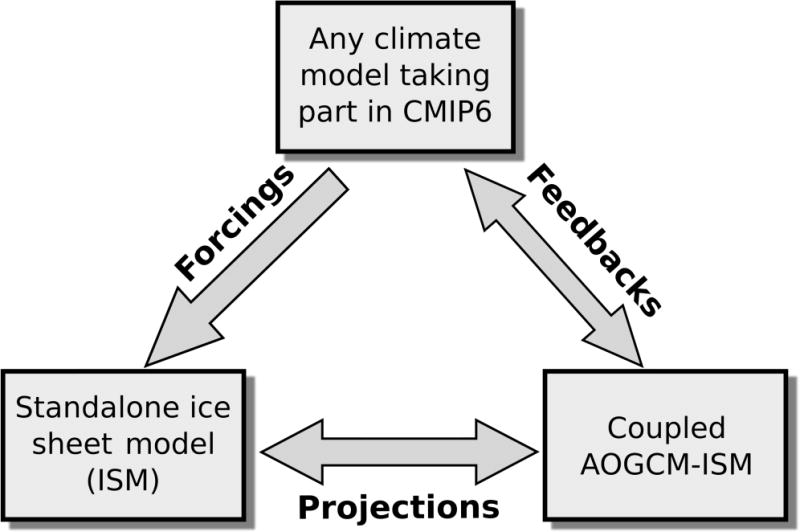
Overview of the ISMIP6 effort designed to obtain forcing from climate models, project sea-level contributions using ice sheet models, and explore ice sheet-climate feedbacks.

3 ISMIP6 Experimental Design

Following the CMIP6 protocol, the ISMIP6 experiments both use and augment the CMIP6-DECK (Diagnostic Evaluation and Characterization of Klima) and Historical simulations (Meehl et al., 2014; Eyring et al., 2016). In addition, ISMIP6 collaborates with the CMIP6-Endorsed Paleoclimate Model Intercomparison effort (PMIP4, Kageyama et al., 2016) and builds on the CMIP6-Endorsed ScenarioMIP (O’Neill et al., 2016) that focuses on future climate experiments for CMIP6. For a selected number of AGCM/AOGCM experiments that are already part of CMIP6 (Table 1 and described in Sect. 3.1), three additional model configurations are proposed: “XXX-withism”, “ism-XXX-self” and “ism-XXX-std”, where XXX stands for different forcing scenarios as described later and shown in Table 2. The first case, “XXX-withism”, indicates that the ice sheet model is run interactively with the climate model (the AOGCM-ISM configuration described in Sect. 3.2). The other two cases describe an offline, or “standalone”, ice sheet model that is driven by outputs from either an uncoupled AOGCM “ism-XXX-self” (the ISM configuration described in Sect. 3.2) or from a standard ISMIP6 dataset “ism-XXX-std” that will be provided for the glaciology community (the ISM configuration described in Sect. 3.3). The goal of the ism-XXX-self simulations is to obtain an ice sheet evolution and sea-level contribution that can be compared to the AOGCM-only and the AOGCM-ISM experiments in order to gain insight into the feedbacks between ice sheets and climate. Differences between the ism-XXX-self runs and AOGCM-ISM runs will be attributable to ice-sheet feedbacks on other climate components. The ism-XXX-std experiments will complement the AOGCM and AOGCM-ISM experiments by using ice sheet configurations and forcing data sets that are as realistic as possible, aiming to minimize the effects of AOGCM biases. The ism-XXX-std simulations target mainly the glaciology community and aim to simulate realistic ice-sheet evolution for sea-level estimates. A related set of standalone experiments, called initMIP, will explore uncertainties associated with the initialization of ice sheet models for Greenland and Antarctica.

Table 1.

Overview of the experiments with climate models not coupled with ice sheet models that are to be used by ISMIP6. All experiments are started on 1 January and end on 31 December of the specified years.

Experiment	CMIP6 label (experiment_id)	Experiment description	Start year	End year	Minimum no. years per simulation	Major purposes
DECK experiments
AMIP	amip	Observed SSTs and SICs prescribed	1979	2014	36	Evaluation, variability
Pre-industrial control	piControl	Coupled atmosphere-ocean pre-industrial control	n/a	n/a	500	Evaluation, unforced variability
1% yr−1 CO2 concentration increase	1pctCO2	CO2 concentration prescribed to increase at 1% yr−1	n/a	n/a	150	Climate sensitivity, feedbacks, idealized benchmark
Extension of 1pctCO2, needed to generate 1pctCO2to4x
Extension from year 140 of 1pctCO2 with 4 time CO2	1pctCO2-4xext	Branched from 1pctCO2 run at year 140 and run with CO2 fixed at quadruple pre-industrial concentration	n/a	n/a	210	Climate sensitivity, feedbacks, idealized benchmark
CMIP6 historical simulation
Past ~ 1.5 centuries	historical	Simulation of the recent past	1850	2014	165	Evaluation
CMIP6-Endorsed ScenarioMIP simulations
SSP5-8.5	ssp585	Future scenario with high radiative forcing by the end of the century	2015	2100	86	Climate sensitivity
SSP5-8.5ext	ssp585	Extension of high radiative forcing future scenario	2101	2300	200	Climate sensitivity
CMIP6-Endorsed PMIP4 simulation
PMIP4 last interglacial	lig127k	Equilibrium simulation of the peak of the last interglacial period	127ka	n/a	100	Climate sensitivity, feedbacks, long responses

Table 2.

Overview of the ISMIP6 experiments with dynamic ice sheets that are either coupled to climate models (AOGCMISM, XXX-withism) or run offline (ISM, ism-XXX-self and ism-XXX-std). All experiments are started on 1 January and end on 31 December of the specified years. PD indicates that the start date correspond to the date of the present-day ISM spin-up.

Experiment	CMIP6 label (experiment_id)	Experiment description	Start year	End year	Minimum no. years per simulation	Starting conditions	Tier
Repeat of DECK experiments with dynamic ice sheets
AMIP	ism-amip-std	Offline ISM forced by ISMIP6-specified AGCM amip output	PD	2014	n/a	ISM spinup	2
Pre-industrial control	piControl-withism	Pre-industrial control with interactive ice sheet	n/a	n/a	500	AOGCM-ISM spinup	1
	ism-piControl-self	Offline ISM forced by own AOGCM piControl output	n/a	n/a	500	AOGCM-ISM spinup	1
Present-day control	ism-pdControl-std	Offline ISM forced by end of present-day spinup conditions	n/a	n/a	100	ISM spinup	1
Repeat of 1pctCO2to4x with dynamic ice sheets
1% yr−1 CO2 concentration increase to 4 time CO2	1pctCO2to4x-withism	Simulation with interactive ice sheet forced by 1% yr−1 CO2 increase to 4× CO2 (subsequently held constant to quadruple levels)	n/a	n/a	350	AOGCM-ISM spinup	1
	ism-1pctCO2to4x-self	Offline ISM forced by own AOGCM 1pctCO2to4x output	n/a	n/a	350	AOGCM-ISM spinup	1
	ism-1pctCO2to4x-std	Offline ISM forced by ISMIP6-specified AOGCM 1pctCO2to4x output	n/a	n/a	350	ISM spinup	1
Repeat of CMIP6 historical simulation with dynamic ice sheets
Past ~ 1.5 centuries	historical-withism	Historical simulation with interactive ice sheets	1850	2014	165	AOGCM-ISM spinup	2
	ism-historical-self	Offline ISM forced by own AOGCM historical output	1850	2014	165	AOGCM-ISM spinup	2
	ism-historial-std	Offline ISM forced by ISMIP6-specified AOGCM historical output	PD	2014	n/a	ISM spinup	2
Repeat of CMIP6-Endorsed ScenarioMIP simulations with dynamic ice sheets
High radiative forcing future emission scenario (SSP5-8.5)	ssp585-withism	SSP5-8.5 simulation with interactive ice sheet	2015	2100	86	historical-withism	2
	ism-ssp585-self	Offline ISM forced by own AOGCM ssp585 output	2015	2100	86	ism-historical-self	2
	ism-ssp585-std	Offline ISM forced by ISMIP6-specified AOGCM ssp585 output	2015	2100	86	ism-historical-std	2
Extension of high radiative forcing future scenario (SSP5-8.5ext)	ssp585-withism	Extension of SSP5-8.5 simulation with interactive ice sheet	2101	2300	200	ssp585-withism	3
	ism-ssp585-self	Offline ISM forced by own AOGCM ssp585 output	2101	2300	200	ism-ssp585-self	3
	ism-ssp585-std	Offline ISM forced by ISMIP6-specified AOGCM ssp585 output	2101	2300	200	ism-ssp585-std	3
Last interglacial simulation based on PMIP4 simulations with standalone ice sheet only
Last interglacial	ism-lig127k-std	Last interglacial simulation forced by lig127k and other PMIP experiments.	135ka	115ka	20000	ISM spinup	3
initMIP Greenland and Antarctic simulations with standalone ice sheet only
Present-day control	ism-ctrl-std	Present-day control	n/a	n/a	100	ISM spinup	1
Surface mass balance	ism-asmb-std	Surface mass balance anomaly prescribed	n/a	n/a	100	ISM spinup	1
Basal melt	ism-bsmb-std	Basal melt anomaly under floating ice prescribed (Antarctica only)	n/a	n/a	100	ISM spinup	1

3.1 Analysis of experiments with climate models proposed elsewhere in CMIP6 (and not coupled to ISMs)

A first component of the ISMIP6 effort is to assess and evaluate CMIP atmosphere general circulation models (AGCMs) and coupled atmosphere – ocean general circulation models (AOGCMs) over and surrounding the polar ice sheets. This part of ISMIP6 can be viewed as diagnostic in the sense that all climate models that participate in CMIP6 will be included in this assessment without requiring extra work from the climate modeling centers. These experiments do not include dynamic ice sheets, and as explained in the CMIP6 protocol (Eyring et al., 2016), climate modeling centers that contribute to CMIP6 are required to submit simulations for the DECK and CMIP6 Historical runs. Our goals are to establish the suitability of the CMIP models for producing climate input for ice sheet models and to assess the uncertainty in projections of sea-level change arising from such climate input. As described in Sect. 4, an additional goal is to assess past and projected changes in surface forcing (here for a fixed ice-sheet extent and topography), along with the resulting sea-level contribution from both ice sheets due to changes in surface freshwater flux alone. The largest uncertainty in century-scale sea-level projections, however, remains the dynamic ice sheet response to changes in atmospheric and oceanic conditions, which will be addressed by the other components of ISMIP6 (Sect. 3.2 and 3.3).

The experiments with climate models not coupled to ISMs, listed in Table 1, are central to ISMIP6 and thus briefly introduced. These AGCM/AOGCM experiments are already part of CMIP6, such that more detailed information on the experimental protocol is available elsewhere in this special issue. ISMIP6 uses three of the four DECK experiments described in Eyring et al. (2016). The Atmospheric Model Intercomparison Project (amip, Gates et al., 1999) simulation allows the evaluation of the atmospheric component of climate models given prescribed sea-surface temperatures and sea ice conditions. These oceanic forcings are based on observations and range from January 1979 to December 2014 for CMIP6 (see Appendix A1.1 of Eyring et al., 2016). The pre-industrial control, piControl, is a coupled atmospheric and oceanic simulation with constant conditions, chosen to represent pre-industrial values (with 1850 as the reference year, see Appendix A1.2 of Eyring et al., 2016). piControl serves as the starting point for many simulations and is meant to capture the pre-industrial quasi-equilibrium state of the climate system. It allows an evaluation of model drift and provides insight into the unforced internal variability. The DECK also contains two idealized “climate change” experiments, in which the CO₂ concentration is varied to gain insight into the Earth system response to basic greenhouse gas forcing. ISMIP6 will focus on a 1pctCO2to4x simulation, a slightly modified version of the DECK 1pctCO2 simulation. The 1pctCO2 simulation is 150 years long, starting from the piControl, with a 1% per year increase in atmospheric CO₂ concentration. The 1pctCO2to4x simulation is identical to 1pctCO2 for the first 140 years, at which point the CO₂ concentration reaches four times the initial value. At this point, 1pctCO2to4x branches from 1pctCO2 and continues with constant quadrupled CO₂. (Note that the 1pctCO2to4x scenario was called 1pctCO2 in CMIP5 (Taylor et al., 2012) and 1pctto4x in CMIP3.) In order to produce boundary conditions for their ism-1pctCO2to4x-self simulation, groups participating in ISMIP6 with a coupled AOGCMISM should carry out a 1pctCO2-4xext simulation, which starts from year 140 of their 1pctCO2 simulation and runs for a minimum of 210 years (and ideally 360 years, see Sect 3.2) with CO₂ concentration held fixed. The 1pctCO2to4x fields will not be stored in the CMIP6 archive, but can be generated by merging the outputs from the first 140 years of the 1pctCO2 run with that from 1pctCO2-4xext.

The CMIP6 Historical simulation, historical, tests the capability of AOGCMs to simulate the historical period, defined as 1850 to 2014. The forcing is derived from observations of solar variability and changes in atmospheric composition, including both anthropogenic and volcanic sources (see Appendix A2 of Eyring et al., 2016). The more distant past is the focus of PMIP4, which designs paleoclimate experiments (Kageyama et al., 2016; Otto-Bliesner et al., 2016). ISMIP6 collaborates with PMIP4 for experiment lig127k, a simulated time slice of the Last Interglacial (LIG): the warm period from 129,000 to 116,000 years ago when global mean sea level was 5–10 m higher than present (Masson-Delmott et al., 2013). The future in CMIP6 falls under the guidance of ScenarioMIP (O’Neill et al., 2016), ISMIP6 will focus on the high-emission scenario ssp585 that produces a radiative forcing of 8.5 W m⁻² in 2100 and its extension to 2300, to evaluate climate and ice sheet changes in response to a large forcing. If time permits, lower-emission mitigation scenarios will also be included in the ISMIP6 standalone ice sheet framework.

Evaluation of the climate over and surrounding the ice sheets is necessary both to establish the suitability of current climate models to provide forcing for ice sheet models, and to gain insight into sea-level uncertainty arising from uncertainty in atmospheric and oceanic climate forcings. Of particular interest is the surface climate over the ice sheets, with a focus on temperature and surface mass balance (SMB). SMB is defined as total precipitation minus evaporation, sublimation and surface runoff, where runoff is meltwater less any refreezing within the snowpack. Because the ocean condition is prescribed for the amip simulation but not for the historical simulation, we expect that the temperature and SMB provided by the two simulations over the same time period will differ. We will explore our second interest, the capability of climate models to reproduce the oceanic state in the vicinity of the ice sheets, using the historical simulation.

The general approach for evaluating the atmospheric component of climate models over the ice sheets (e.g., Yoshimori and Abe-Ouchi, 2012; Fettweis et al., 2013; Vizcaíno et al., 2013; Cullather et al., 2014; Lenaerts et al., 2016) is to compare the large-scale atmospheric state over the polar regions, the local climate, and processes at the ice-sheet surface. The latter focuses on whether the climate model can simulate snow processes, including albedo evolution and refreezing, at a horizontal resolution that captures the SMB gradients at ice sheet margins. Both the atmospheric components and factors that can affect atmospheric processes are often evaluated. One example is determining whether sea ice conditions are adequately captured in historical simulations (e.g., Lenaerts et al., 2016), as sea ice can influence moisture availability and therefore precipitation. However, adequate modeling of precipitation also requires well-resolved ice sheet topography (orographic forcing), which remains challenging for coarse-resolution climate models (Vizcaíno, 2014).

The large-scale atmospheric state over the polar regions is often assessed by comparing the modeled atmospheric flow at 500 hPa to atmospheric reanalysis values. For the local climate, near-surface winds and near-surface temperatures can be compared to regional climate models (RCM) such as RACMO2 (van Meijgaard et al., 2008; Lenaerts et al., 2012; van Angelen et al., 2014), MAR (Fettweis, 2007; Fettweis et al., 2011), or HIRHAM (Langen et al., 2015; Lucas-Picher et al., 2012), reanalysis (e.g., Agosta et al., 2015), and observations where available. RCMs are also used to evaluate the spatial pattern of surface mass balance and its components (precipitation, sublimation, and surface melt) computed by global circulation models. The surface energy budget, particularly the seasonal cycle of net shortwave and longwave radiation and the sensible and latent heat fluxes, can be evaluated against measurements taken by automatic weather stations on the ice sheet surface. Such stations include, for example, the 15 Greenland stations known as the GC–Net (Steffen and Box, 2001), the Greenland PROMICE network with a focus on the ablation zone (Ahlstrom et al., 2008), and in Antarctica the Neumayer Base (Lenaerts et al., 2010). These stations also record winds and temperatures. The surface temperature over the ice sheets may also be evaluated from satellite observations, using, for example, data derived from the Moderate Resolution Imaging Spectroradiometer (MODIS, Hall et al., 2012). These remotely sensed temperature products show the onset and/or spatial extent of surface melt (e.g., Mote et al., 1993; Hall et al., 2013), which can then be used to assess whether the climate models capture the relevant processes at the ice sheet surface (e.g., Fettweis et al., 2011; Cullather et al., 2016). However, a full understanding of why surface melt varies from model to model may require investigations that include cloud properties (van Tricht et al., 2016).

The current generation of climate models participating in CMIP6 is unlikely to simulate ocean circulation in ice shelf cavities or within fjords. Thus, evaluation of the ocean state around the ice sheets involves first establishing that the climate models can reproduce certain properties of the key water masses. Ocean circulation around the Greenland Ice Sheet involves a complex interaction between polar waters of Arctic origin and Atlantic waters from the subtropical North Atlantic (Straneo et al., 2012). The mechanisms that transport warm water through fjords and toward the ice fronts remain an active area of research (Wilson and Straneo, 2015; Straneo and Cenedese, 2015). In the Southern Ocean, important water masses include Antarctic Bottom Water and Antarctic Intermediate Waters. In the coastal regions, Circumpolar Deep Water, Antarctic Surface Water, and High Salinity Shelf Water are the primary oceanic influences on ice sheets (Bracegirdle et al., 2016). Given the difficulty many CMIP5 models had in capturing high-latitude ocean properties, CMIP6 models should be evaluated using existing datasets (Bracegirdle et al., 2016). These datasets include Argo, expendable bathythermograph (XBT) and conductivity/temperature/depth (CTD) vertical temperature and salinity profiles (e.g., Dong et al., 2008), sea ice extent products sourced from passive microwave instruments (e.g., Bjorgo et al., 1997; Cavalieri and Parkinson, 2012; Parkinson and Cavalieri, 2012), sea surface temperature (SST) from WindSat and AMSR-E over the open ocean, satellite altimetry (Jason-1 and Jason-2) over the open ocean, and World Ocean Atlas 2009 climatological temperatures. For ocean models that include ice-shelf cavities and ice/ocean interactions, sub-ice-shelf basal melting can be compared with glaciological estimates of ice-shelf melting around Antarctica (Rignot et al., 2013; Depoorter et al., 2013) derived from remote-sensing observations, as well as independent tracer-oceanographic estimates (Loose et al., 2009; Rodehacke et al., 2006). Just as regional atmospheric models will be key for evaluating the atmospheric component of climate models, regionally focused ocean models (e.g., Timmermann et al., 2012) and ocean reanalysis products (e.g. Menemenlis et al., 2008) are likely to provide valuable insight for evaluating CMIP ocean models.

3.2 Experiments with climate models coupled to ISMs

The second component of ISMIP6 is a suite of experiments designed to assess the impacts of dynamic ice sheets on climate and to better understand feedbacks between ice sheets and climate. We also aim to obtain an ensemble of sea-level projections from fully coupled atmosphere – ocean – ice sheet frameworks, which can later be compared to projections from standalone ice sheet models (Sect. 3.3). The experiments should be identical to the corresponding standard CMIP AOGCM experiments except for the treatment of ice sheets, so that any observed feedbacks and impacts can be attributed to dynamic ice sheets and not to other sources. As indicated in Table 2, four coupled AOGCM-ISM simulations are proposed, whose experiment IDs are piControl-withism, 1pctCO2to4x-withism, historical-withism and ssp585-withism. These simulations are complemented by four ISM simulations: ism-piControl-self, ism-1pctCO2to4x-self, ism-historical-self and ism-ssp585-self.

In the XXX-withism setup, the ice sheet model is run interactively with the AOGCM: the climate model sends a surface forcing (SMB at a minimum) to the ice sheet model, and receives changes in ice sheet geometry. The land surface type and surface elevation in the climate model are dynamic, allowing, for example, a reduced albedo if the land surface changes from glaciated to unglaciated. Changes in the ice sheet mass should also affect the ocean temperature and salinity, as freshwater fluxes (liquid and/or solid) and energy fluxes are routed to the ocean. Liquid fluxes can originate from surface runoff, subglacial drainage systems, or basal melting of the ice in contact with the ocean. Solid fluxes come from iceberg calving, which may be computed with calving laws whose details are left to the discretion of the modeling groups. Explicit iceberg models are not required. Similarly, ocean melting of ice shelves can be handled as desired, as long as the net freshwater flux and latent heat flux are routed consistently to the ocean model.

The ism-XXX-self configuration denotes runs of an uncoupled ice sheet model driven by the outputs of the AOGCM-only simulation (Sect. 3.1). The ism-XXX-self experiment is only meaningful in combination with a completed XXX-withism, and with the same combination of climate and ice sheet models. In this configuration, changes in the ice sheet do not affect the climate model, and therefore the climate inputs passed to the ice sheet model differ from those in the AOGCM-ISM experiment. The ice sheet model should, however, be configured with the same settings as for the AOGCM-ISM runs and should use the same initial conditions (i.e., the outcome of the spin-up carried out with the coupled AOGCM-ISM).

Initial conditions for both the ism-XXX-self experiments and the XXX-withism experiments will be generated by running the coupled AOGCM-ISM to a quasi-equilibrium state with pre-industrial forcing that represent year 1850. Pre-industrial AOGCM-ISM spin-up is an area of active research (e.g., Fyke et al. 2014) that seeks to produce a consistent non-drifting coupled state corresponding to the pre-industrial climate, which is different from the contemporary state (Kjeldsen et al., 2015). The challenge is that ice sheets reach quasi-equilibrium on timescales of many millennia, more slowly than the oceans, which typically have been the slowest components of AOGCMs. To reach steady state, the ice sheet model may have to be run for ~10,000 years or longer. Since runs of this length are impractical for a complex climate model, the coupling between the ice sheet model and the climate model will likely have to be asynchronous for at least part of the spin-up. In this case, once the ice sheet model has reached steady state, the coupled system should be run synchronously for an additional period before starting the experiments. ISMIP6 will not dictate spin-up procedures for obtaining pre-industrial initial ice-sheet conditions, but the procedure should be documented.

Ideally, the ice sheet model should be forced with the actual SMB computed by the climate model, rather than an SMB corrected to match observed climatology. We accept that there may be biases in the atmospheric or land models that can lead to an unrealistic SMB, which could result in a steady-state ice sheet geometry that differs substantially from present-day observations. However, correcting for these biases can distort the feedbacks between ice sheets and climate that we seek to investigate. We hope to learn from and ultimately reduce these biases, in the same way that biases elsewhere in the simulated coupled climate system are reduced by greater understanding and improved model design. On the other hand, if the geometry of the spun-up ice sheet is greatly different from observations, then the initial ice sheet for the ism-XXX-self experiments may be far from steady state with the SMB forcing from the standard, uncoupled AOGCM. As a result, the ism-XXX-self experiment could have a large drift that obscures the climate signal. The drift will be quantified from the control experiments. In case of a large drift, or if the spun-up ice sheet in the coupled system is deemed to be too unrealistic, an alternative spin-up method would be to apply SMB anomalies from the AOGCM, superposed on a climatology that yields more realistic equilibrium ice sheet geometry.

The method used to downscale SMB (as well as oceanic forcing) from the coarse climate model grid to the finer ice sheet model grid is left to the discretion of each group, but should be well documented. The data request for ISMIP6 in Appendix A asks modelers to report certain fields on both the atmospheric and ice sheet grids to allow for an evaluation of the downscaling procedure. Also, ISMIP6 prefers that the surface-melt component of SMB be obtained from an energy-based method that conserves mass and energy, to facilitate interpretation of the drivers of SMB variability and change (e.g. Vizcaíno, 2014). Highly parameterized methods of computing surface melt, such as positive-degree-day (PDD) methods (e.g. Reeh, 1991; Bougamont et al., 2007), should be avoided. The choice of the ice sheet model, its complexity in approximating ice flow, and ice-sheet-relevant boundary conditions (e.g., geothermal flux) are left to the modelers’ discretion. In all experiments, however, the ice sheets should not be forced to terminate at the present-day ice margin if the simulated SMB and/or the ice sheet dynamics cause a margin advance.

Regardless of the spin-up method, the first ISMIP6 experiment to be performed with the coupled AOGCM–ISM is the pre-industrial control, piControl-withism. This is a multi-century (500 years suggested) control run aiming to assess model drift and systematic bias and to capture unforced natural variability. The drift in the standalone ISM experiments ism-XXX-self will be quantified with a control run (ism-piControl-self). The core ISMIP6 prognostic climate change experiment is 1pctCO2to4x-withism, which applies a 1% per year increase in CO₂ concentrations over 140 years until levels are quadrupled, then holds concentrations fixed for an additional two to four centuries. The 1pctCO2to4x-withism will be compared to the AOGCM simulation 1pctCO2to4x (the first 140 years of the DECK 1pctCO2 merged with the 1pctCO2-4xext) and to ism-1pctCO2to4x-self (the standalone ISM forced by the AOGCM surface mass balance and temperature from 1pctCO2to4x). The duration of these three experiments should be the same. It is suggested that the experiments be run for at least 350 years, and if possible for 500 years, because previous studies (e.g., Ridley et al., 2005; Vizcaíno et al., 2008; 2010) indicate that coupled AOGCM–ISM runs start to clearly diverge from uncoupled runs after about 250–300 years of simulation.

Another set of experiments repeats the CMIP6 historical and ssp585 simulations with a coupled AOGCM-ISM. The historical-withism simulation begins at year 1850 from the pre-industrial spin-up and finishes at the end of 2014. This simulation is followed by ssp585-withism, with experimental settings and forcings as described in O’Neill et al. (2016). The ssp585-withism begins in January 2015 and is initiated from the December 2014 results of the historical-withism simulation. The ssp585-withism experiment is run for the 21^st century and its extension to the end of the 23^rd century. For completeness, these experiments are to be repeated with standalone ISM simulations ism-historical-self and ism-ssp585-self. We accept that with this protocol, the 2015 ice sheet is likely to be distinct from the observed ice sheet due to model drift from the Historical run, and that this will have implications for projected ice sheet evolution (e.g., Stone et al., 2010).

Based on community feedback, we expect that several AOGCM–ISMs will be ready to participate in coupled climate experiments for CMIP6. Table 3 shows climate modeling centers that have expressed interest in participating in ISMIP6. The primary focus is coupled ice-sheet–atmosphere simulation for the Greenland Ice Sheet, but some groups have indicated participation only in the diagnostic aspect of ISMIP6 (where the goal is to provide climate data for the standalone ice sheet work). Full coupling of ice sheet models to climate models remains challenging, especially for interactions with the ocean. Accurate treatment of ice-ocean interactions requires ISMs that can simulate grounding line migration (which demands fine grid resolution) and iceberg calving, and ocean models that can simulate circulation in the cavities below ice shelves and the consequent melting or accretion of ice on the undersides of the shelves. Accurate treatment of ice-ocean interactions will likely also require ocean models to alter their domain (both vertically and horizontally) as the calving front migrates and as sub-ice-shelf ocean cavities evolve in space and time. For the Greenland Ice Sheet, ocean models may need to capture fjord dynamics on smaller spatial scales (~1 km) than are currently resolved by global ocean models. In addition, credible ice-ocean coupling requires accurate knowledge of the bathymetry beneath ice shelves and ice sheets, where data are sparse. Because of these challenges, we do not expect a realistic treatment of the Antarctic Ice Sheet in the ISMIP6 coupled AOGCM-ISM experiments. Antarctica is included, however, in the standalone experiments described in the next section.

Table 3.

Climate Modeling Centers that have expressed an interest in ISMIP6.

Climate Model	Ice Sheet Model	Institute/Country
CanESM*	None	CCCma/CA
CESM2	CISM	NCAR-LANL/USA
CNRM-CM	GRISLI	CNRM-CERFACS/FR
EC-Earth	GrIS	DMI/DK
GISS	PISM	NASA-GISS/USA
INMCM	VUB	INM/RU
IPSL-CM6	GRISLI	IPSL/FR
MIROC-ESM	IcIES	AORI-UT-JAMSTEC-NIES/JP
MPI-ESM	PISM	MPI/DE
UKESM	BISICLES	MetOffice/UK

^*Indicates only an interest in the diagnostic component (no AOGCM-ISM participation anticipated).

3.3 Experiments with ISMs not coupled to climate models

The final set of ISMIP6 experiments will use standalone ice sheet models driven by climate model output and other datasets. Groups and models that have expressed an interest in participating in this aspect of ISMIP6 are listed in Table 4. The models participating in this effort will likely be configured differently from those in the ism-XXX-self simulations described in Sect. 3.2. For example, an ice sheet model that is spun up to quasi-equilibrium with a climate model will likely have a thickness and extent that differ appreciably from observed values, whereas standalone models can be initialized more realistically. Also, an ISM in a climate model might use a coarse resolution or a simple approximation of ice dynamics in order to be more computationally efficient, while the same model used strictly for projections would likely have a finer resolution, at least in regions of fast flow (e.g. Aschwanden et al., 2016), and could incorporate more complex ice flow dynamics. Similarly, ice sheet models that are used for paleoclimate studies are often distinct from those used for projections of a few hundred years.

Table 4.

Ice sheet modeling groups that have expressed an interest in ISMIP6.

Ice Sheet Model	Greenland	Antarctica	Institute/Country
BISICLES	x		BGC/UK
CISM	x		LANL/NCAR/USA
Elmer/Ice	x	x	LGGE/FR
f.ETISH	x	x	ULB/BE
GISM	x		VUB/BE
GRISLI	x		LSCE/FR
IcIES	x	x	MIROC/JP
IMAUICE	x	x	IMAU/NL
ISSM	x	x	JPL/USA
ISSM	x	x	UCI/USA
ISSM	x		AWI/DE
MPAS-LI		x	LANL/ORNL/USA
PennState3D		x	PSU/USA
PISM	x		UAF/USA
PISM	x	x	ARC/NZ
PISM	x		DMI/DK
PISM	x		MPIM/DE
SICOPOLIS	x	x	ILTS/JP
SICOPOLIS	x	x	PIK/DE
Úa		x	BAS/UK
WAVI		x	BAS/UK

x Indicates planned contribution.

3.3.1 initMIP

The initMIP ice sheet experiments are designed to explore uncertainties in sea-level projections associated with model initialization and spin-up. Such uncertainties have been identified by previous model intercomparison efforts (e.g., Bindschadler et al., 2012; Nowicki et al., 2013a, b; Edwards et al., 2014a, Shannon et al., 2013; Goelzer et al., 2013; Gillet-Chaulet et al., 2012) and include the impacts of model initial conditions, sub-grid scale processes, and poorly known parameters. The initMIP project aims to evaluate initialization procedures, to estimate trends caused by model initializations and to investigate the impact of choices in numerical and physical parameters (e.g., stress balance approximation or model resolution). Results of the initMIP project are expected to point to specific aspects of ice sheet initialization that have a crucial impact on sea-level projections and may be improved.

ISM initialization methods to present-day conditions range from running paleo-climate spin-up for thousands of years (e.g., Martin et al., 2011; Sato and Greve, 2012; Aschwanden et al., 2013; Fürst et al., 2015; Saito et al., 2016) to assimilating present-day observations (e.g., Morlighem et al., 2010; Gillet-Chaulet et al., 2012; Seroussi et al., 2013, Arthern et al., 2015). The choices made in this procedure affect ice sheet extent, flow rates, volume, and volume trends, which can have substantial effects on estimates of ice sheet contribution to sea-level rise (e.g. Aðalgeirsdóttir et al., 2014). Improving ISM initial conditions is an active area of research and a multidisciplinary effort. It requires acquisition of additional data with high spatial coverage over entire ice sheets and at increased resolution (e.g., Bamber et al., 2013; Rignot et al., 2011b; Joughin et al., 2010a; Howat et al., 2014). Ideally, all datasets used in the data assimilation are from the same period, as initializing an ice sheet model with datasets taken at different times can cause the ice flow model to artificially redistribute the glacier mass in unrealistic ways that serve only to reconcile these inconsistencies (Seroussi et al., 2011). This also implies that the date associated with the initial state can differ between models based on the data sets used. New algorithms that reconcile initialization datasets are being developed, most notably for bedrock elevation (e.g., Morlighem et al., 2011; Morlighem et al., 2014), which is notoriously poorly constrained.

The initMIP project consists of a Greenland component and an Antarctic component. Following initialization, there is a set of two forward experiments for the Greenland Ice Sheet and three forward experiments for the Antarctic Ice Sheet, each run for at least 100 years: i) a control run (ism-ctrl-std), ii) a surface mass balance anomaly run (ism-asmb-std) and iii) a basal melt anomaly run (ism-abmb-std) in which anomalous melt is applied beneath the floating portion of the Antarctic Ice Sheet. All other model parameters and forcing in the forward runs are the same as those used for initialization. The ism-ctrl-std is an unforced forward experiment designed to evaluate the initialization procedure and characterize model drift, the surface mass balance remaining identical to the one used during the initialization procedure. In ism-asmb-std, a prescribed SMB anomaly is applied to test the model response to a large perturbation. The schematic perturbation anomaly mimics outputs of several SMB models of different complexity between the end of the 20^th century and the end of the 21^th century, and is designed to capture the first-order pattern of SMB changes expected from climate models. The schematic SMB anomalies are defined everywhere on the model grid, and are therefore applicable for models with varying ice sheet extent. In ism-abmb-std, a prescribed anomaly of basal melting rate under floating ice is applied while SMB is kept the same as in ism-ctrl-std. Because of the difference in ice shelf extent between the different models, the basal melt anomaly is prescribed to be constant for each basin. This scalar value is different for each basin and derived from the mean values of the ice shelf melt observed by Rignot et al. (2013) and Depoorter et al. (2013). The applied anomaly simulates a doubling of sub-ice-shelf melting after 40 years of simulation for models with initial melting rates close to today’s observations.

Since these experiments are designed to allow comparison among the different models, some simplifications are imposed. Neither SMB nor bedrock topography should be adjusted in response to ice-sheet geometric changes in these forward experiments. However, to sample the uncertainty in sea-level due to initialization, groups are encouraged to submit multiple variations of the experiment, for example by changing the sliding law, stress balance approximation, model resolution, or datasets (such as using different bedrocks). While the initialization procedures used by the different participating groups are not prescribed by ISMIP6, it is expected that individual groups will take advantage of the initMIP results to improve their initialization procedures. initMIP is also intended to give ice sheet modelers an opportunity to get involved in ISMIP6 at an early stage, before outputs of CMIP6 AOGCM become available; hence our prescription of simplified anomalies. We refer interested readers to the initMIP webpage (http://www.climate-cryosphere.org/wiki/index.php?title=InitMIP) for more information.

3.3.2 ism-XXX-std configuration

The ism-XXX-std experiments target primarily the glaciology community and seek to obtain realistic ice sheet evolution to inform estimates of past, present and future sea level. ISMIP6 will supply forcing data from CMIP6 that allows standalone ISMs to simulate the evolution of both the Greenland and Antarctic Ice Sheets. ISMIP6 seeks to assess the uncertainty in sea-level change arising from both the ice sheet models and the climate forcing. A key concern is that ISMIP6 assess uncertainty associated with emission scenario and the AOGCMs’ simulation of these scenarios: for a given emission scenario, the AOGCMs simulation of this scenario will result in a range of atmospheric and oceanic forcings. Clearly, there is a tension between the range of potential ice sheet forcing, the need to explore uncertainty associated purely with ISMs (e.g., related to initial conditions, bedrock topography and parametric uncertainty), and the computing requirements of specific ISMs (some of which may only be able to perform a small number of experiments). To this end, we anticipate identifying a subset of forcing from the CMIP6 AOGCM ensemble based on the analysis of AOGCM simulations of ice-sheet climate (Sect. 3.1). The subset will be chosen to capture the full range of potential ice sheet forcing for a given emission scenario, using metrics of the SMB and ocean forcing to investigate that range. Within the selected subset of forcing, we plan to identify a small number of simulations that all ISMs must perform. Groups that are able to perform numerous simulations will be encouraged to participate in all experiments. Shannon et al. (2013) is an example of this approach.

The forcing data can naturally be divided into atmospheric and oceanic forcing. Central to the former is the means to determine SMB associated with a particular CMIP6 experiment. Several methods have previously been employed to do this. Until we can assess the quality of the climate simulated by CMIP6 AOGCMs above and around the ice sheets (after the analysis of the CMIP6 DECK and Historical simulations), a definitive choice cannot be made. However, we list the options in order of preference:

1. Use the SMB calculated by the AOGCM directly. This has the advantage that the SMB will be entirely consistent with other parts of that AOGCM’s simulation of climate. There is concern, however, that the quality of the SMB computed by the AOGCMs will make this approach unrealistic due primarily to the mismatch between the spatial resolution of AOGCMs and the characteristic length scale of variations in SMB. Several groups have, however, made recent progress in this area (e.g., Vizcaíno et al., 2013; Lipscomb et al., 2013). The use of anomalies should also be considered in this context.

2. In the event that AOGCM-determined SMB is shown to be inadequate, an intermediate step is required. Previously, this has been the use of Regional Climate Models (RCMs) to simulate SMB. For example, the ice2sea effort chose to generate SMB from an RCM (Edwards et al., 2014a,b; Fettweis et al., 2013). This approach, however, introduces a further link into the processing chain that may lead to delay in the production of sea-level projections. It also introduces the issue of choice of RCM and whether results from a number of RCMs should be used (further complicating the design of the ISM ensemble). Furthermore, the use of RCMs as intermediaries between AOGCMs and ISMs adds ambiguity about which biases are introduced by the AOGCMs and which biases are the result of the RCMs.

3. Use a parameterization or simplified process model to simulate SMB by downscaling atmospheric forcing over the ice sheet from an AOGCM. This approach was used by SeaRISE (Bindschadler et al., 2013), where the precipitation and surface temperature from 18 AOGCMs models taking part in the A1B scenario were combined to generate monthly mean values. These mean precipitation and temperature values were then passed to the SMB scheme of the ice sheet model (generally a PDD method that accounted for the temperature aspect of the SMB-elevation feedback) to obtain SMB anomalies that were added to the ice sheet surface conditions at initialization.

A further consideration is that the AOGCM models assume a fixed ice sheet elevation: i.e., they neglect the effect of ice sheet elevation change on the atmosphere and hence omit the SMB-elevation feedback. Standalone ISMs will need to include this effect by parameterizing the SMB lapse rate (Edwards et al., 2014a,b; Fettweis et al., 2013; Goelzer et al., 2013). This approach may be less of an issue for method 3 above because SMB is determined interactively within the ISM rather than being prescribed as forcing.

A second way in which the atmosphere could force dynamic change in ice sheets is through the production of large quantities of melt water. Mechanisms have been proposed that link melt water to both ice shelf collapse (Banwell et al., 2013) and enhanced lubrication of ice flow (Zwally et al., 2002) (although recent modeling studies suggest a minor influence of the latter on large-scale ice flow (e.g., Shannon et al., 2013)). Surface air temperature and runoff forcing will therefore also be made available.

Both Antarctica and Greenland are thought to respond to changes in proximal ocean temperatures, which affect the melt rates of floating ice shelves and the vertical faces of outlet glaciers. Obtaining suitable oceanic forcing from CMIP6 climate models will be a major challenge. Few CMIP6 models will calculate the appropriate melt rates, and even these results are likely to be inaccurate because of issues of model resolution and the unique physics of ocean circulation adjacent to melting ice. Melt rates will therefore need to be determined outside the climate model using an index for proximal ocean temperature. This index is most likely to be water temperature (and salinity) at the continental shelf break at an intermediate range of depths (equivalent to the base of ice shelves or the depth of ice grounded on bedrock). This quantity will be included in our evaluation of CMIP6 forcing (see Sect. 3.1).

A wide range of approaches has been used to calculate the required melt rate from prescribed ocean-temperature forcing. The simplest method is to calculate melt rate anomalies from changes in the nearest ocean temperature using an observationally derived relation of 10 m yr⁻¹ °C⁻¹ (Rignot and Jacobs, 2002). However, this linear relation between ocean temperature and melt rates is calibrated for melt rates at the grounding line, and likely is missing important non-linearities (Holland et al., 2008). An alternative approach is to parameterize melt rates as proportional to the difference between ocean temperature at the shelf break and the freezing temperature at the ice shelf base. Beckman and Goosse (2003) developed such a scheme for ocean models, and similar schemes have been applied in offline ice sheet model simulations with idealized ocean forcing (e.g., Martin et al., 2011; Pollard and DeConto, 2012; DeConto and Pollard, 2016). In those studies, the ocean temperature is set to the average temperature between 200 and 600 m depth (Martin et al., 2011), or the temperature at 400 m depth (DeConto and Pollard, 2016), or specified differently for specific Antarctic sectors (Pollard and DeConto, 2012). Depending on the evaluation of the CMIP6 models, ISMIP6 may adapt one of these choices, or could prescribe depth-varying profiles of ocean temperature (and possibly salinity). The dependence of melt rates on thermal driving ranges from linear (Martin et al., 2011) to quadratic (Pollard and DeConto, 2012; DeConto and Pollard, 2016). Since the freezing temperature at the ice base decreases with depth, the melt rates in all schemes tend to be higher near grounding lines, as found from observations.

If none of the CMIP6 ocean models can accurately capture the broad-scale polar ocean circulation or produce realistic near-shelf temperatures, an alternative is to prescribe a melt rate that simply depends on the ice shelf draft (e.g. Joughin et al., 2010b; Favier et al., 2014). This approach is less satisfactory, however, as it ignores temporal changes in ocean conditions, and typically uses coefficients calibrated to local thermal conditions. If ISMIP6 uses this approach, the provided coefficients would not be uniform, but would take into account that ocean waters reaching ice shelf cavities or fronts differ regionally. In Antarctica, for example, the ice shelves of Pine Island Glacier and Thwaites Glaciers lie in “warm” water, while the Filchner-Ronne or Ross ice shelves reside in “cold” water. Ocean temperatures reflect the dominant water sources, with warm waters dominated by circumpolar deep waters (Jacobs et al., 2011), while cold waters typically correspond to high- salinity shelf water (Nichols et al., 2001).

Ice-ocean interactions are an active area of research, and more sophisticated parameterizations of melt are becoming available (e.g., Jenkins, 2016; Asay-Davis et al., 2016). Simplified models of the system could be used (e.g., Payne et al., 2007), as could high-resolution ocean models that resolve ice-shelf cavities and fjords. Given this wide range of methods, ISMIP6 will leave the detailed choice of the parameterization to individual ice-sheet modelers, but will issue guidance on what constitutes an acceptable parameterization. We will organize workshops with the polar ocean community to investigate how to best derive oceanic forcing for ice sheet models, so that by the time the CMIP6 ocean models are evaluated, a clearer protocol is in place. The calculated melt rate will be part of the standard data request for ice sheet models (see Appendix A), and part of our evaluation will be to determine how well the applied forcing compares to observed melt rates of Rignot et al. (2014) and Depoorter et al. (2014).

ISMIP6 will not dictate the choice of ice sheet model complexity in terms of the ice flow approximation, the basal sliding law, the treatment of grounding lines, the calving law, the ice-sheet-specific boundary conditions (e.g., bedrock topography), or the initialization method. An exception is that models of the Antarctic Ice Sheet should include floating ice shelves and grounding line migration. The spatial resolution of the ISM in the vicinity of fast-flowing ice streams and the grounding line affects the dynamic response (Durand et al., 2009; Pattyn et al., 2012, 2013), and the model resolution must be fine enough to capture this response accurately. To this end, participating models are encouraged to take part in model intercomparison efforts that target specific aspects of ice sheet modeling, such as the current MISOMIP (Marine Ice Sheet–Ocean Model Intercomparison Project; Asay-Davis et al., 2016) and are required to take part in initMIP (initialization-focused experiments that compare and evaluate the simulated present-day state; Sect. 3.3.1). The lack of a stricter protocol is a reflection of the challenges in identifying which factors are the most important when making projections, which datasets are most accurate, and how to best capture and parameterize certain ice-sheet processes. For example, although the choice of bedrock topography affects mass transport and is thus likely to influence a projection, it is currently not possible to identify a best dataset due to the difficulty in obtaining bedrock measurements. Groups are encouraged to repeat the experiments with a variety of perturbations of weakly constrained parameters, boundary conditions, etc. in order to test the sensitivity of projections to these choices.

Unlike the protocol for climate models, the ism-XXX-std simulations cannot be initiated from a spin-up corresponding to year 1850. This is due to the challenge of initializing ice sheet models to pre-industrial conditions, which are constrained more weakly than the contemporary state: the quantity of accurate, high-resolution data available during the satellite era far exceeds that available for pre-industrial and historical periods. The majority of ice sheet models use these data in sophisticated initialization and assimilation procedures, such that the present-day state of the ice sheet is simulated with high fidelity. The lack of suitable data before the satellite era means that no such accuracy can be assumed for simulations of the historical periods. Such inaccuracies are known to have a large effect on projections. For instance, discrepancies between projections can often be attributed to slight differences in the geometry (e.g., Shannon et al. 2013). The ism-XXX-std simulations will thus be initiated from a present-day spin-up.

The first ism-XXX-std simulation is ism-pdControl-std, the ice sheet present-day control with constant forcing needed to evaluate model drift. This constant forcing is based on the climate at the end of the initialization procedure. For many models, the forcing and simulation will be the same as the ism-ctrl-std in the initMIP experiment (Sect. 3.3.1), unless a change has been made in the initialization. The idealized climate change experiment, ism-1pctCO2to4x-std, considers a 1% per year atmospheric CO₂ concentration rise until quadrupled concentrations and stabilization thereafter. The ism-historical-std will be an abbreviated simulation for the historical period (as it begins from the present-day spin-up) and, following the CMIP6 protocol, ends in December 2014. The ism-amip-std is a simulation for the last few decades to understand the well-observed record of ice sheet changes. The results from the ism-amip-std and ism-historical-std are likely to differ, and the comparison will provide some insight into the relative importance of biases, climate variability and climate change. The main simulation for projecting 21^st century sea-level rise is the ism-ssp585-std, which is initiated from the ism-historical-std simulation. (As mentioned previously, other scenarios will be considered if time permits.) If possible, projections should continue to the end of the 23^rd century.

We complement the experiments for the recent past and future with one paleo experiment (ism-lig127k-std), to simulate Greenland ice-sheet evolution during the Last Interglacial. The transient simulation will span the period 135 kyr to 115 kyr to include transitions from the preceding and to the following cold periods. The climate forcing for ism-lig127k-std will be derived from the PMIP4-CMIP6 experiment lig127k and other (transient) LIG climate simulations (cf. Bakker et al., 2012; Lunt et al., 2013) that will be performed by PMIP4 (Otto-Bliesner et al., 2016). The proposed experiment builds on past efforts to study Greenland ice-sheet stability and evolution during the LIG and constrain the Greenland contribution to the LIG sea-level highstand (e.g. Robinson et al., 2011; Born and Nisancioglu, 2012; Helsen et al., 2013).

3.4 Prioritization of experiments and timing

The ISMIP6 experiments listed in Table 2 are divided into three “Tiers” to indicate prioritization. Tier 1 denotes experiments that are to be completed by the ISMIP6 participants. Tier 2 experiments are highly encouraged, while Tier 3 experiments are optional.

For the coupled AOGCM-ISM experiments, the Tier 1 experiments piControl-withism and 1pctCO2to4x-withism should be performed first. These experiments have already been performed by many climate modeling groups, and their idealized settings allow for an easier evaluation of the ice-climate feedback. The Tier 2 experiments, historical-withism and ssp585-withism, are more relevant to our goal of producing sea-level projections concurrent with the CMIP6 future climate. Ideally, the XXX-withism and ism-XXX-self experiments would follow the corresponding AOGCM experiments with no more than a six-month lag.

For the standalone ism-XXX-std experiments, ISMIP6 is constrained by the timing of the AOGCM runs that will be used to derive forcings for ice sheets. We anticipate that the DECK simulations will not be completed before spring of 2017, which implies that climate models cannot be evaluated rigorously before summer 2017, and in turn that the ISM Tier 1 experiments based on CMIP6 DECK forcing would begin in 2018. As soon as suitable forcings are available from the SSP5-8.5 experiments (CMIP6-Endorsed ScenarioMIP, Tier 1), ism-ssp585-std will be the focus of the standalone ISM work. To allow ice-sheet modeling groups the necessary time to perform the simulations, we plan to begin ism-ssp585-std in early 2019. Similarly, the ism-lig127k-std cannot proceed until the PMIP participants have completed the CMIP6-Endorsed PMIP4 Tier 1 experiment and other transient PMIP4 experiments. In the meantime, ISMIP6 standalone ice sheet models will focus on initMIP, with the goal of finishing this suite of experiments by the end of 2016 for Greenland and by the end of 2017 for Antarctica.

4 Evaluation and Analysis

The framework described in this paper entails an evaluation of the climate system, with a particular focus on the polar regions. This framework works toward the goals of i) assessing the effect of including dynamic ice sheets in climate models and ii) improving confidence in projections of sea-level rise associated with mass loss from the Greenland and Antarctic Ice Sheets. Our evaluation and analysis will be based on key model output variables for the atmosphere, ocean and ice sheets that form the ISMIP6 data request summarized in Appendix A.

4.1 Evaluation of ice sheet models

Ice sheet models will be evaluated using methodologies already in use by the ice-sheet modeling community. These metrics typically begin by assessing whether the volume and area of the modeled present-day ice sheet are comparable to observed values. The next step evaluates the spatial patterns of surface elevation, ice sheet thickness, surface velocities, and positions of the ice front and grounding line. Some ice sheet models are initialized using data assimilation methods, which precludes the use of certain observations in the evaluation. Evaluation of these models can be done by hindcasting, a method that evaluates whether recent observed trends are captured (Aschwanden et al., 2013). Examples include comparison against the gravimetry (GRACE) time series from 2003 onwards, which provides an integrated set of measurements for mass changes in Greenland and Antarctica. This approach will also enable a direct comparison between predicted sea-level rise from ISMs and the change in ocean mass observed by GRACE. The recent IMBIE effort (Ice Sheet Mass Balance Inter-comparison Exercise, Shepherd et al., 2012) facilitates this comparison by combining observations from gravimetry, altimetry and velocity changes between 1992-2012 into a single dataset of annual mass budget for each ice sheet. The follow-on effort, IMBIE2 (Shepherd, personal communication), will extend the record in time and plans to separate the observed mass change into SMB and dynamic components.

4.2 Effects of dynamic ice sheets on climate

The combination of coupled AOGCM-ISM simulations (XXX-withism) and standalone ice sheet simulations (ism-XXX-self) will support a clean analysis of ice-sheet feedbacks on the climate system, which can further affect ice-sheet evolution (e.g., Driesschaert et al., 2007; Goelzer et al., 2011; Vizcaíno et al., 2008, 2010, 2015). A limited number of feedbacks can be studied in an AOGCM without a dynamic ISM. For instance, because AOGCMs generally compute ice-sheet SMB through a land model coupled on hourly time scales to the atmospheric model, the albedo-melt feedback can be studied in an AOGCM alone. Other important feedbacks, however, are present only if the ice sheet is dynamic:

• As ice sheets thin, the lower elevation leads to warmer surface temperatures that increase melting. This ice-elevation feedback is small on sub-century time scales (Edwards et al., 2014b), but over longer time scales, it can drive ice sheets to a point of no return, where retreat would continue unabated even if the climate returned to an unperturbed state.

• Changes in ice sheet elevation modify the regional atmospheric circulation (e.g., Ridley et al., 2005), which can either enhance or slow the rate of retreat.

• Changes in land surface cover (e.g., from glaciated to vegetated) can darken and warm the surface, promoting atmospheric warming and further melting.

• Increased freshwater fluxes (both solid and liquid) from retreating ice sheets can modify the density structure of the ocean, possibly suppressing convection and weakening the Atlantic meridional overturning circulation. Although some studies (e.g., Hu et al., 2009) find that this is a small effect, others suggest that increased runoff from the Greenland Ice Sheet has already reduced deep convection in the Labrador Sea (Yang et al., 2016).

• The buoyancy of fresh glacial meltwater from sub-ice-shelf melting can modify the ocean circulation that drives the melting. On longer time scales, changes in the size and shape of sub-shelf cavities may also alter the circulation.

The ISMIP6 experiments will be performed on climate model runs lasting several centuries, long enough to allow a detailed analysis of at least the first four of these feedbacks. Ocean cavity feedbacks, however, may require further development of ocean models that can adjust their boundaries dynamically as marine ice sheets advance and retreat.

4.3 Sea-level change

The SMB over the Greenland Ice Sheet is currently becoming less positive, thus resulting in an increasing contribution to sea-level rise due to increased surface runoff (van Angelen et al., 2014; Fettweis et al., 2011). This trend is expected to continue (Fettweis et al., 2013; Rae et al., 2012), although there is a large spread in AOGCMs (Yoshimori and Abe-Ouchi, 2012). The picture is less clear for the Antarctic Ice Sheet, where both accumulation and surface melt are projected to increase (Lenaerts et al., 2016). The multi-model ensemble of the surface freshwater flux from AOGCM simulation will provide insight into the resulting contribution of past and future sea level due to changes in SMB alone.

The largest uncertainty in sea level, however, remains the dynamic contribution from the ice sheets. ISMIP6 targets the contribution of dynamic ice sheets to global sea level, via multi-model ensemble analysis of standalone ice sheet models (ism-XXX-std). For a number of experiments, the multi-model ensemble from the ism-XXX-std will be contrasted to the multi-model ensemble resulting from coupled AOGCM-ISM simulations (ism-XXX-withism). We expect the results of the standalone modeling (ism-ssp585-std) to be more robust for projections, as we anticipate that the spun-up ice sheet from the coupled historical simulation (historical-withism) will differ substantially from present-day observations, and these differences will alter the projected ice sheet evolution (e.g., Stone et al., 2010; Shannon et al., 2013). The projections from ssp585-withism will likely expose issues resulting from coupling dynamic ice sheet models to climate models, motivating the community to begin resolving them.

We also aim to quantify the uncertainty in sea level arising from uncertainties in both the ice sheet models and the climate input, hence the need to sample across scenarios and models. For example, the ongoing initMIP project will provide insight into sea-level uncertainties resulting from ice sheet model initialization. By repeating model runs with different datasets, sliding laws, model resolutions, etc., initMIP will allow us to constrain the sea-level contribution associated with these choices. Ice sheet evolution will also depend on climatic drivers. For instance, given a certain number of AOGCMs that simulate present-day ice-sheet SMB reasonably well, comparing their SMB results under various climate-change simulations will allow us to quantify climate-model-driven uncertainty in SMB. If relationships between large-scale climate drivers (e.g., regional temperature and precipitation) and ice-sheet area-integral SMB can be established (e.g., Gregory and Huybrechts, 2006; Fettweis et al., 2013), this would allow estimation of SMB from AOGCM experiments for other climate scenarios. If possible, synergies with other CMIP6 efforts will allow us to further investigate the uncertainty in climate input. For example, the CMIP6-Endorsed High Resolution Model Intercomparison Project (HighResMIP, Haarsma et al., 2016) and Coordinated Regional Climate Downscaling Experiment (CORDEX, Gutowski et al., 2016) may allow us to quantify the impacts of increased resolution on SMB.

5 Discussion and conclusion

ISMIP6 has an experimental protocol and a diagnostic protocol. The experimental design uses and builds upon the core DECK and CMIP6 Historical simulations, along with selected CMIP6-Endorsed PMIP4 and ScenarioMIP simulations. The suite of ISMIP6 experiments involves three types of models: AOGCM/AGCM with no dynamic ice sheets, coupled AOGCM-ISM, and standalone ISM. The diagnostic protocol is based on ice-sheet-related model outputs, many of which are already present in the CMIP6 atmosphere and ocean diagnostics. The evaluation of the climate in the polar regions from AOGCM and AOGCM-ISM simulations will guide recommendations for existing and new ice-sheet–climate coupling efforts. ISMIP6 promotes the development of the ice sheet component of climate models in an effort to bring both climate and ice-sheet models to greater maturity. ISMIP6 targets two of the WCRP Grand Science Challenges: “Melting Ice and Global Consequences” and “Regional Sea-level Change and Coastal Impacts”. Given the current rapid changes in the Greenland and Antarctic Ice Sheets, ice sheets no longer be considered passive players in the climate system. Their contributions to future sea level will likely have considerable human and environmental impacts, and ISMIP6 will facilitate research in this critical area.

ISMIP6 will coordinate simulation and analysis of ice sheet evolution in a changing climate. Inclusion of ice sheet models is unique in CMIP history and is necessary to advance understanding of the sea-level contribution from the Greenland and Antarctic Ice Sheets, the climate system response to ice-sheet changes, and the feedbacks between ice sheets and climate. ISMIP6 is thus an important step in closing the gap between the climate and ice-sheet modeling communities. Our key output, the sea-level contribution from ice sheets, complements the projections of ocean thermal expansion that already sit within the CMIP framework. This improvement will help sea level join the family of variables for which CMIP can provide routine IPCC-style projections. Ultimately, the success of ISMIP6 relies on the broad participation of the CMIP6 modeling centers, standalone ice sheet modeling groups, and analysts of the atmosphere, ocean and ice sheets.

Data availability

The model output from the simulations described in this paper will be distributed through the Earth System Grid Federation (ESGF) with digital object identifiers (DOIs) assigned. In order to document CMIP6’s scientific impact and enable ongoing support of CMIP, users are obligated to acknowledge CMIP6, the participating modeling groups, and the ESGF centers (see details on the CMIP Panel website at http://www.wcrp-climate.org/index.php/wgcm-cmip/about-cmip). Datasets for natural and anthropogenic forcings are required to run the experiments; these datasets are described in separate invited contributions to this Special Issue. The forcing datasets will be made available through the ESGF with version control and DOIs assigned. Exceptions in the distribution method will be made for the forcing for the initMIP Greenland and Antarctic efforts that specifically target standalone ice sheet models. Instruction of how to obtain forcing datasets not available through ESGF will be posted on the ISMIP6 website (http://www.climate-cryosphere.org/activities/targeted/ismip6).

Appendix A: Variable Request

This special issue includes a manuscript that is dedicated to the CMIP6 data request. The majority of our data request is based on the CMIP5 CMOR tables Amon (Monthly Mean Atmopsheric Fields), Omon (Monthly Mean Ocean Fields), LImon (Monthly Mean Land Cryosphere Fields), and OImon (Monthly Mean Ocean Cryosphere Fields), which already contained many of the output required to diagnose and intercompare the climate over land ice/ice sheets and to derive forcing for the ice sheets. In the CF convention, ‘land ice’ comprises grounded ice sheets, floating ice shelves, glaciers and ice caps, while ‘ice sheet’ refers to grounded ice sheets and floating ice shelves. A few additional variables are needed to properly derive the forcings for ice sheets from AOGCMs, and to record outputs from the evolving ice sheets in the coupled AOGCM-ISMs experiments (such as ice elevation change), or from the standalone ice sheet simulations. In this Appendix, we briefly outline the ISMIP6 data request on the atmosphere grid (Table A1), ocean grid (Table A2), and ice sheet grid (Table A3), and provide some context for key new variables.

The mass change of ice sheets (see Fig. A1) is a result of the surface mass balance (SMB), ice melt (or refreeze) at the base of the grounded ice sheet (BMB), and mass exchange with the ocean. The latter can be further split into frontal mass balance (FMB, defined as iceberg calving and melt (or refreeze) at the ice shelf front) and melt (or refreeze) at the base of ice shelves (BMB). All fluxes are defined as positive when the process adds mass to the ice sheet and negative otherwise. The thermal state of the ice sheet models is documented by the basal temperature and by the temperature at the ice sheet-snowpack interface. Note that BMB and basal temperature are computed differently depending on whether the ice is grounded or floating, requiring the use of distinct Long Names, but same Standard Names in Table A3.

Climate models will be evaluated primarily based on how well they can simulate SMB over the ice sheets. This quantity (see Vizcaíno (2014) and Fig. A2) can be defined as precipitation minus runoff minus evaporation (which in our context includes any sublimation, a small term over ice sheets), where precipitation is the sum of snowfall and rainfall. Runoff is the liquid water that escapes the ice sheet, while some of the water may be retained in the snow pack and possibly refreezes. The evaluation of climate models also benefits from analysis of energy fluxes, key temperatures, and area fraction of land ice, grounded ice sheet (excludes ice shelf) and snow over the land ice. Note that some variables, such as SMB, are present in both Table A1 and Table A3, since in a coupled AOGCM-ISM simulation, the two will differ due to downscaling to the ice sheet grid. The data request for the ocean serves primarily as input to construct oceanic forcing for ice sheet models off-line. It is not as extensive as the data request for the atmosphere, because marine boundary conditions for outlet glaciers and ice shelves are not routinely generated by AOGCMs. It is therefore premature to set diagnostic protocols at this stage. However, participants are asked to follow the protocols of the CMIP6-Endorsed Ocean Model Intercomparison Project (OMIP, Griffies et al., 2016) when preparing the data listed in Table A2, in particular when regridding the ocean data from a native grid to the CMIP6 standard grids. The ice sheet data request contains key characteristics needed to evaluate the ice sheet geometry, and ice sheet flow. It also contains key ice sheet specific boundary conditions that may differ between models and a record of the forcing applied to the ice sheet model. To facilitate the analysis of the ice sheet contribution to sea level, a number of integrated measures (for example, ice sheet mass) are also requested.

Figure A1.

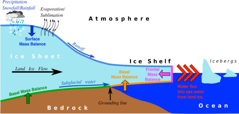
Illustration of the mass change of ice sheets and key processes that are specific to ice sheet model evaluation or forcing. See text for details.

Figure A2.

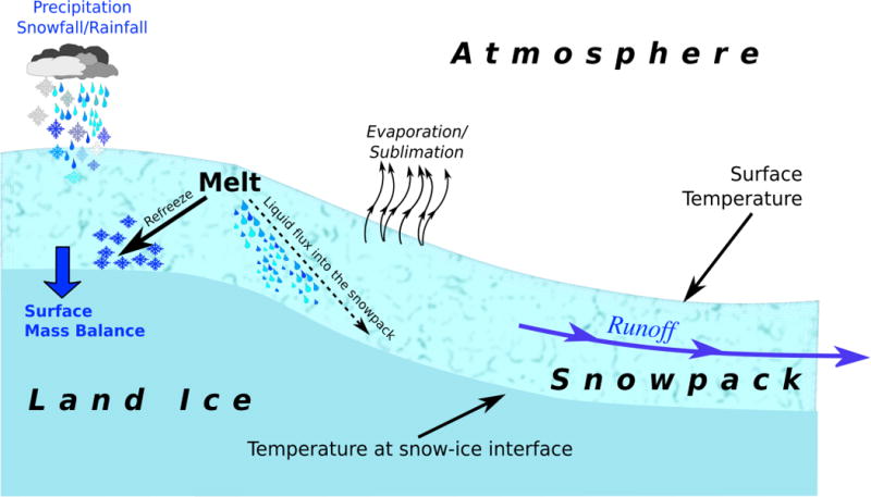
Illustration of key processes needed to compute atmospheric forcing for ice sheet models, and to evaluate the surface mass balance simulated by climate models.

Table A1.

Data in the LImon Table (Monthly Mean Land Cryosphere Fields) and/or Amon Table (Monthly Mean Atmospheric Fields) needed to capture the glaciated/ice sheet surface realm. These fields are saved on the atmosphere grid and contain monthly output. Tier indicate priority of variable: Mandatory (1), Desirable (2), Experimental (3). These variables are requested for climate models participating in the diagnostic component of ISMIP6 (Table 1), and for the XXX-withism experiments (Table 2). Flux variables are defined positive when the process adds mass or energy to the ice sheet and negative otherwise.

Long name (netCDF)	Units	Standard name (CF)	Tier
Near surface air temperature (2m)	K	air_temperature	1
Surface temperature	K	surface_temperature	1
Snow internal temperature	K	temperature_in_surface_snow	2
Temperature at the top of ice sheet model	K	temperature_at_top_of_ice_sheet_model	2
Surface mass balance flux	kg m−2 s−1	land_ice_surface_specific_mass_balance_flux	2
Snowfall flux	kg m−2 s−1	snowfall_flux	1
Rainfall flux	kg m−2 s−1	rainfall_flux	2
Surface snow and ice sublimation flux	kg m−2 s−1	surface_snow_and_ice_sublimation_flux	2
Surface snow and ice melt flux	kg m−2 s−1	surface_snow_and_ice_melt_flux	2
Surface snow melt flux	kg m−2 s−1	surface_snow_melt_flux	3
Surface ice melt flux	kg m−2 s−1	land_ice_surface_melt_flux	3
Surface snow and ice refreezing flux	kg m−2 s−1	surface_snow_and_ice_refreezing_flux	3
Land ice runoff	kg m−2 s−1	land_ice_runoff_flux	2
Snow area fraction	1	surface_snow_area_fraction	1
Land ice area fraction	1	land_ice_area_fraction	1
Grounded ice sheet area fraction	1	grounded_ice_sheet_area_fraction	1
Floating ice shelf area fraction	1	floating_ice_shelf_area_fraction	1
Land ice altitude	m	surface_altitude	1
Net latent heat flux over land ice	W m−2	surface_upward_latent_heat_flux	1
Sensible heat flux over land ice	W m−2	surface_upward_sensible_heat_flux	1
Downwelling shortwave	W m−2	surface_downwelling_shortwave_flux_in_air	1
Upward shortwave over land ice	W m−2	surface_upwelling_shortwave_flux_in_air	1
Downwelling longwave	W m−2	surface_downwelling_longwave_flux_in_air	1
Upward longwave over land ice	W m−2	surface_upwelling_longwave_flux_in_air	1
Albedo over land ice	1	surface_albedo	2

Table A2.

Data on the Omon Tables (Monthly Mean Ocean Fields) needed to capture the glaciated/ice sheet surface realm or for intercomparison of the model simulations. These fields are saved on the ocean grid and contain monthly output. Data preparation should follow the CMIP6-Endorsed OMIP protocol. Tier indicates priority of variable: Mandatory (1), Desirable (2), Experimental (3). These variables are requested for climate models participating in the diagnostic component of ISMIP6 (Table 1), and for the XXX-withism experiments (Table 2). Flux variables are defined positive when the process adds mass to the ocean and negative otherwise.

Long name (netCDF)	Units	Standard name (CF)	Tier
Global surface height above geoid	m	sea_surface_height_above_geoid	1
Global average thermosteric sea-level change	m	global_average_thermosteric_sea_level_change	1
Sea water potential temperature	°C	sea_water_potential_temperature	1
Sea surface temperature	°C	sea_surface_temperature	2
Sea water salinity	Psu	sea_water_salinity	1
Water flux into sea water from iceberg	kg m−2 s−1	water_flux_into_sea_water_from_icebergs	2
Water flux into sea water from ice sheets	kg m−2 s−1	water_flux_into_sea_water_from_land_ice	3

Table A3.

Data on the LImonant, LImongre, LIyrant or LIyrgre Tables needed to capture the dynamical ice sheet model realm. These fields are saved on the ice sheet grid and contain monthly or yearly output. Tier indicate priority of variable: Mandatory (1), Desirable (2), Experimental (3). These variables are requested for models participating in the XXX-withism, ism-XXX-self and ism-XXX-std experiments (Table 2). Flux variables are defined positive when the process adds mass or energy to the ice sheet and negative otherwise.

Long name (netCDF)	Units	Standard name (CF)	Tier
Ice sheet altitude	m	surface_altitude	1
Ice sheet thickness	m	land_ice_thickness	1
Bedrock altitude	m	bedrock_altitude	1
Bedrock geothermal heat flux	W m−2	upward_geothermal_heat_flux_at_ground_level_in_land_ice	3
Land ice calving flux	kg m−2 s−1	land_ice_specific_mass_flux_due_to_calving	3
Land ice vertical front mass balance flux	kg m−2 s−1	land_ice_specific_mass_flux_due_to_calving_and_ice_front_melting	2
Surface mass balance and its components	kg m−2 s−1	see Table A1	1
Basal mass balance of grounded ice sheet	kg m−2 s−1	land_ice_basal_specific_mass_balance_flux	2
Basal mass balance of floating ice shelf	kg m−2 s−1	land_ice_basal_specific_mass_balance_flux	2
X-component of land ice surface velocity	m yr−1	land_ice_surface_x_velocity	1
Y-component of land ice surface velocity	m yr−1	land_ice_ surface_y_velocity	1
Z-component of land ice surface velocity	m yr−1	land_ice_ surface_upward_velocity	2
X-component of land ice basal velocity	m yr−1	land_ice_basal_x_velocity	1
Y-component of land ice basal velocity	m yr−1	land_ice_basal_y_velocity	1
Z-component of land ice basal velocity	m yr−1	land_ice_basal_upward_velocity	2
X-component of land ice vertical mean velocity	m yr−1	land_ice_vertical_mean_x_velocity	2
Y-component of land ice vertical mean velocity	m yr−1	land_ice_vertical_mean_y_velocity	2
Land ice basal drag	Pa	magnitude_of_basal_drag_at_land_ice_base	3
Surface temperature	K	surface_temperature	1
Temperature at the top of ice sheet model	K	temperature_at_top_of_ice_sheet_model	1
Basal temperature of grounded ice sheet	K	temperature_at_base_of_ice_sheet_model	1
Basal temperature of floating ice shelf	K	temperature_at_base_of_ice_sheet_model	1
Land ice area fraction	1	land_ice_area_fraction	1
Grounded ice area fraction	1	grounded_ice_sheet_area_fraction	1
Floating ice sheet area fraction	1	floating_ice_sheet_area_fraction	1
Surface snow area fraction	1	surface_snow_area_fraction	2
Scalar outputs/Integrated measures
Ice mass	kg	land_ice_mass	2
Ice mass not displacing sea water	kg	land_ice_mass_not_displacing_sea_water	2
Area covered by grounded ice	m2	grounded_land_ice_area	3
Area covered by floating ice	m2	floating_ice_shelf_area	3
Total SMB flux	kg s−1	tendency_of_land_ice_mass_due_to_surface_mass_balance	3
Total BMB flux	kg s−1	tendency_of_land_ice_mass_due_to_basal_mass_balance	3
Total calving flux	kg s−1	tendency_of_land_ice_mass_due_to_calving	3

References

- Abe-Ouchi A, Saito F, Kawamura K, Raymo M, Okuno J, Takahashi K, Blatter H. Insolation driven 100.000-year glacial cycles and hysteresis of ice sheet volume. Nature. 2013;500:190–193. doi: 10.1038/nature12374. [DOI] [PubMed] [Google Scholar]
- Aðalgeirsdóttir G, Aschwanden A, Khroulev C, Boberg F, Mottram R, Lucas-Picher P, Christensen JH. Role of model initialization for projections of 21st-century Greenland ice sheet mass loss. Journal of Glaciology. 2014;60:782–794. [Google Scholar]
- Agosta C, Fettweis X, Datta R. Evaluation of the CMIP5 models in the aim of regional modelling of the Antarctic surface mass balance. The Cryosphere. 2015;9:2311–2321. doi: 10.5194/tc-9-2311-2015. [DOI] [Google Scholar]
- Ahlstrøm AP, Gravesen P, Andersen SB, van As D, Citterio M, Fausto RS, Nielsen S, Jepsen HF, Kristensen SS, Christensen EL, Stenseng L, Forsberg R, Hanson S, Petersen D, Team, P. P. A new programme for monitoring the mass loss of the Greenland ice sheet. Copenhagen, Denmark: 2008. Available from: http://www.geus.dk/DK/publications/geol-survey-dk-gl-bull/15/Documents/nr15_p61-64.pdf. [Google Scholar]
- van Angelen JH, van den Broeke MR, Wouters B, Lenaerts JTM. Contemporary 1960–2012 evolution of the climate and surface mass balance of the Greenland ice sheet. Surveys in Geophysics. 2014;35:1155–1174. doi: 10.1007/s10712-013-9261-z. [DOI] [Google Scholar]
- Arthern RJ, Hindmarsh RCA, Williams CR. Flow speed within the Antarctic ice sheet and its controls inferred from satellite observations. J Geophys Res. 2015;120(7):1171–1188. doi: 10.1002/2014JF003239. [DOI] [Google Scholar]
- Asay-Davis XS, Cornford SL, Durand G, Galton-Fenzi BK, Gladstone RM, Gudmundsson GH, Hattermann T, Holland DM, Holland D, Holland PR, Martin DF, Mathiot P, Pattyn F, Seroussi H. Experimental design for three interrelated marine ice sheet and ocean model intercomparison projects: MISMIP v. 3 (MISMIP +), ISOMIP v. 2 (ISOMIP +) and MISOMIP v. 1 (MISOMIP1) Geosci Model Dev. 2016;9:2471–2497. doi: 10.5194/gmd-9-2471-2016. [DOI] [Google Scholar]
- Aschwanden A, Aðalgeirsdóttir G, Khroulev C. Hindcasting to measure ice sheet model sensitivity to initial states. The Cryosphere. 2013;7:1083–1093. doi: 10.5194/tc-7-1083-2013. [DOI] [Google Scholar]
- Aschwanden A, Fahnestock MA, Truffer M. Complex Greenland outlet glacier flow captured. Nat Commun. 2016;7:10524. doi: 10.1038/ncomms10524. [DOI] [PMC free article] [PubMed] [Google Scholar]
- Bakker P, Stone EJ, Charbit S, Gröger M, Krebs-Kanzow U, Ritz SP, Varma V, Khon S, Lunt DJ, Mikolajewicz U, Prange M, Renssen H, Schneider B, Schulz M. Last interglacial temperature evolution - a model inter-comparison. Clim Past Discuss. 2012;8:4663–4699. doi: 10.5194/cpd-8-4663-2012. [DOI] [Google Scholar]
- Bamber JL, Griggs JA, Hurkmans RTWL, Dowdeswell JA, Gogineni SP, Howat I, Mouginot J, Paden J, Palmer S, Rignot E, Steinhage D. A new bed elevation dataset for Greenland. The Cryosphere. 2013;7:499–510. doi: 10.5194/tc-7-499-2013. [DOI] [Google Scholar]
- Banwell AF, MacAyeal DR, Sergienko OV. Breakup of the Larsen B Ice Shelf Triggered by Chain Reaction Drainage of Supraglacial Lakes. Geophys Res Lett. 2013;40:5872–5876. doi: 10.1002/2013GLO57694. [DOI] [Google Scholar]
- Beckmann A, Goosse H. A parameterization of ice shelf–ocean interaction for climate models. Ocean Modelling. 2003;5(2):157–170. [Google Scholar]
- Bindschadler RA, Nowicki S, Abe-Ouchi A, Aschwanden A, Choi H, Fastook J, Granzow G, Greve R, Gutowski G, Herzfeld U, Jackson C, Johnson J, Khroulev C, Levermann A, Lipscomb WH, Martin MA, Morlighem M, Parizek BR, Pollard D, Price SF, Ren D, Saito F, Sato T, Seddik H, Seroussi H, Takahashi K, Walker R, Wang WL. Ice-Sheet Model Sensitivities to Environmental Forcing and Their Use in Projecting Future Sea-level (the SeaRISE Project) J Glaciol. 2013;59:195–224. doi: 10.3189/2013JoG12J125. [DOI] [Google Scholar]
- Bjørgo E, Johannessen OM, Miles MW. Analysis of merged SMMR-SSMI time series of Arctic and Antarctic sea ice parameters 1978–1995. Geophysical Research Letters. 1997;24:413–416. [Google Scholar]
- Born A, Nisancioglu KH. Melting of Northern Greenland during the last interglaciation. Cryosphere. 2012;6:1239–1250. doi: 10.5194/tc-6-1239-2012. [DOI] [Google Scholar]
- Bougamont M, Bamber JL, Ridley JK, Gladstone RM, Greuell W, Hanna E, Payne AJ, Rutt I. Impact of model physics on estimating the surface mass balance of the Greenland ice sheet. Geophys Res Lett. 2007;34 doi: 10.1029/2007GL030700. [DOI] [Google Scholar]
- Box JE, Fettweis X, Stroeve JC, Tedesco M, Hall DK, Steffen K. Greenland ice sheet albedo feedback: thermodynamics and atmospheric drivers. The Cryosphere. 2012;6:821–839. doi: 10.5194/tc-6-821-2012. [DOI] [Google Scholar]
- van den Broeke M, Bamber J, Ettema J, Rignot E, Schrama E, van de Berg WJ, van Meijgaard E, Velicogna I, Wouters B. Partitioning Recent Greenland Mass Loss. Science. 2009;326:984–986. doi: 10.1126/science.1178176. [DOI] [PubMed] [Google Scholar]
- Broecker W. Massive iceberg discharges as triggers for global climate change. Nature. 1994;372:421–424. [Google Scholar]
- Bracegirdle TJ, Bertler NA, Carleton AM, Ding Q, Fogwill CJ, Fyfe JC, Hellmer HH, Karpechko AY, Kusahara K, Larour E, Mayewski PA, Meier WN, Polvani LM, Russell JL, Stevenson SL, Turner J, Wessem JM, van de Berg WJ, Wainer I. A Multidisciplinary Perspective on Climate Model Evaluation For Antarctica. Bulletin of the American Meteorological Society. 2016;97(2):ES23–6. doi: 10.1175/BAMS-D-15-00108.1. [DOI] [Google Scholar]
- Calov R, Ganopolski A, Kubatzki C, Claussen M. Mechanisms and time scales of glacial inception simulated with an Earth system model of intermediate complexity. Clim Past. 2009;5:245–258. doi: 10.5194/cp-5-245-2009. [DOI] [Google Scholar]
- Cavalieri DJ, Parkinson CL. Arctic sea ice variability and trends, 1979–2010. The Cryosphere. 2012;6:881–889. doi: 10.5194/tc-6-881-2012. [DOI] [Google Scholar]
- Church JA, Gregory JM. Changes in Sea Level. In: Intergovernmental Panel on Climate Change, editor. Climate Change 2001: The Scientific Basis. Cambridge University Press; Cambridge: 2001. (co-ordinating lead authors with 34 other authors) [Google Scholar]
- Church JA, Clark PU, Cazenave A, Gregory JM, Jevrejeva S, Levermann A, Merrifield MA, Milne GA, Nerem RS, Nunn PD, Payne AJ, Pfeffer WT, Stammer D, Unnikrishnan AS. Sea-level Change. Climate Change 2013 The Physical Science Basis. In: Stocker TF, Qin D, Plattner G-K, Tignor M, Allen SK, Boschung J, Nauels A, Xia Y, Bex V, Midgley PM, editors. Contribution of Working Group I to the Fifth Assessment Report of the Intergovernmental Panel on Climate Change. Cambridge University Press; Cambridge, United Kingdom and New York, NY, USA: 2013. [Google Scholar]
- Cullather RI, Nowicki SM, Zhao B, Suarez MJ. Evaluation of the surface representation of the Greenland Ice Sheet in a general circulation model. Journal of Climate. 2014;27:4835–4856. [Google Scholar]
- Cullather R, Nowicki S, Zhao B, Koenig L. A characterization of Greenland Ice Sheet surface melt and runoff in contemporary reanalyses and a regional climate model. Frontiers in Earth Science. 2016;4:10. [Google Scholar]
- DeConto RM, Pollard D. Contribution of Antarctica to past and future sea-level rise. Nature. 2016;531:591–597. doi: 10.1038/nature17145. [DOI] [PubMed] [Google Scholar]
- Depoorter MA, Bamber JL, Griggs JA, Lenaerts JTM, Ligtenberg SRM, van den Broeke MR, Moholdt G. Calving fluxes and basal melt rates of the Antarctic ice shelves. Nature. 2013;502:89–93. doi: 10.1038/nature12567. [DOI] [PubMed] [Google Scholar]
- Driesschaert E, Fichefet T, Goosse H, Huybrechts P, Janssens I, Mouchet A, Munhoven G, Brovkin V, Weber S. Modeling the influence of Greenland ice sheet melting on the Atlantic meridional overturning circulation during the next millennia. Geophys Res Lett. 2007;34(10):10707. [Google Scholar]
- Durand G, Gagliardini O, Zwinger T, Le Meur E, Hindmarsh RC. Full Stokes modeling of marine ice sheets: influence of the grid size. Annals of Glaciology. 2009;50:109–114. [Google Scholar]
- Dong S, Sprintall J, Gille ST, Talley L. Outhern Ocean mixed-layer depth from Argo float profiles. Journal of Geophysical Research: Oceans. 2008;113:C06013. doi: 10.1029/2006JC004051. [DOI] [Google Scholar]
- Edwards TL, Fettweis X, Gagliardini O, Gillet-Chaulet F, Goelzer H, Gregory JM, Hoffman M, Huybrechts P, Payne AJ, Perego M, Price S, Quiquet A, Ritz C. Probabilistic parameterisation of the surface mass balance– elevation feedback in regional climate model simulations of the Greenland ice sheet. The Cryosphere. 2014a;8:181–194. doi: 10.5194/tc-8-181-2014. [DOI] [Google Scholar]
- Edwards TL, Fettweis X, Gagliardini O, Gillet-Chaulet F, Goelzer H, Gregory JM, Hoffman M, Huybrechts P, Payne AJ, Perego M, Price S, Quiquet A, Ritz C. Effect of uncertainty in surface mass balance–elevation feedback on projections of the future sea-level contribution of the Greenland ice sheet. The Cryosphere. 2014b;8:195–208. doi: 10.5194/tc-8-195-2014. [DOI] [Google Scholar]
- Enderlin EM, Howat IM, Jeong S, Noh MJ, Angelen JH, van den Broeke MR. An improved mass budget for the Greenland ice sheet. Geophys Res Lett. 2014;41:866–872. [Google Scholar]
- Eyring V, Bony S, Meehl GA, Senior CA, Stevens B, Stouffer RJ, Taylor KE. Overview of the Coupled Model Intercomparison Project Phase 6 (CMIP6) experimental design and organization. Geosci Model Dev. 2016;9:1937–1958. doi: 10.5194/gmd-9-1937-2016. [DOI] [Google Scholar]
- Favier L, Durand G, Cornford SL, Gudmundsson GH, Gagliardini O, Gillet-Chaulet F, Zonger T, Payne T, Le Brocq AM. Retreat of Pine Island Glacier controlled by marine ice-sheet instability. Nature Climate Change. 2014;4:117–121. doi: 10.1038/nclimate2094. [DOI] [Google Scholar]
- Fettweis X. Reconstruction of the 1979–2006 Greenland ice sheet surface mass balance using the regional climate model MAR. The Cryosphere. 2007;1:21–40. doi: 10.5194/tc-1-21-2007. [DOI] [Google Scholar]
- Fettweis X, Tedesco M, van den Broeke M, Ettema J. Melting trends over the Greenland ice sheet 1958–2009 from spaceborne microwave data and regional climate models. The Cryosphere. 2011;5:359–375. doi: 10.5194/tc-5-359-2011. [DOI] [Google Scholar]
- Fettweis X, Franco B, Tedesco M, van Angelen JH, Lenaerts JTM, van den Broeke MR, Gallée H. Estimating the Greenland ice sheet surface mass balance contribution to future sea-level rise using the regional atmospheric climate model MAR. The Cryosphere. 2013;7:469–489. doi: 10.5194/tc-7-469-2013. [DOI] [Google Scholar]
- Fricker HA, Scambos T, Bindschadler R, Padman L. An active subglacial water system in West Antarctica mapped from space. Science. 2007;315:1544–1548. doi: 10.1126/science.1136897. [DOI] [PubMed] [Google Scholar]
- Fürst JJ, Durand D, Gillet-Chaulet F, Merino N, Tavard L, Mouginot J, Gourmelen N, Gagliardini O. Assimilation of Antarctic velocity observations provides evidence for uncharted pinning points. The Cryosphere. 2015;9(4):1427–1443. doi: 10.5194/tc-9-1427-2015. [DOI] [Google Scholar]
- Fyke JG, Sacks WJ, Lipscomb WH. A technique for generating consistent ice sheet initial conditions for coupled ice sheet/climate models. Geosci Model Dev. 2014;7:1183–1195. doi: 10.5194/gmd-7-1183-2014. [DOI] [Google Scholar]
- Gates WL, Boyle JS, Covey C, Dease CG, Doutriaux CM, Drach RS, Fiorino M, Gleckler PJ, Hnilo JJ, Marlais SM, Phillips TJ, Potter GL, Santer BD, Sperber KR, Taylor KE, Williams DN. An overview of the results of the Atmospheric Model Intercomparison Project (AMIP I) B Am Meteorol Soc. 1999;80:29–55. [Google Scholar]
- Gillet-Chaulet F, Gagliardini O, Seddik H, Nodet M, Durand G, Ritz C, Zwinger T, Greve R, Vaughan DG. Greenland ice sheet contribution to sea-level rise from a new-generation ice-sheet model. The Cryosphere. 2012;6:1561–1576. doi: 10.5194/tc-6-1561-2012. [DOI] [Google Scholar]
- Goelzer H, Huybrechts P, Loutre MF, Goosse H, Fichefet T, Mouchet A. Impact of Greenland and Antarctic ice sheet interactions on climate sensitivity. Clim Dyn. 2011:1–14. doi: 10.1007/s00382-010-0885-0. [DOI] [Google Scholar]
- Goelzer H, Huybrechts P, Fürst JJ, Nick FM, Andersen ML, Edwards TL, Fettweis X, Payne AJ, Shannon S. Sensitivity of Greenland ice sheet projections to model formulations. J Glaciol. 2013;59:733–549. doi: 10.3189/2013JoG12J182. [DOI] [Google Scholar]
- Gregory JM, Huybrechts P. Ice-sheet contributions to future sea-level change, Philosophical Transactions of the Royal Society of London A: Mathematical. Physical and Engineering Sciences. 2006;364:1709–1732. doi: 10.1098/rsta.2006.1796. [DOI] [PubMed] [Google Scholar]
- Griffies SM, Danabasoglu G, Durack PJ, Adcroft AJ, Balaji V, Böning CW, Chassignet EP, Curchitser E, Deshayes J, Drange H, Fox-Kemper B, Gleckler PJ, Gregory JM, Haak H, Hallberg RW, Hewitt HT, Holland DM, Ilyina T, Jungclaus JH, Komuro Y, Krasting JP, Large WG, Marsland SJ, Masina S, McDougall TJ, Nurser AJG, Orr JC, Pirani A, Qiao F, Stouffer RJ, Taylor KE, Treguier AM, Tsujino H, Uotila P, Valdivieso M, Winton M, Yeager SG. Experimental and diagnostic protocol for the physical component of the CMIP6 Ocean Model Intercomparison Project (OMIP), Geosci. Model Dev Discuss. 2016 doi: 10.5194/gmd-2016-77. in review. [DOI] [Google Scholar]
- Gutowski WJ, Jr, Giorgi F, Timbal B, Frigon A, Jacob D, Kang HS, Krishnan R, Lee B, Lennard C, Nikulin G, O’Rourke E, Rixen M, Solman S, Stephenson T, Tangang F. WCRP COordinated Regional Downscaling EXperiment (CORDEX): A diagnostic MIP for CMIP6, Geosci. Model Dev. 2016;9:4087–4095. doi: 10.5194/gmd-9-4087-2016. [DOI] [Google Scholar]
- Haarsma RJ, Roberts M, Vidale PL, Senior CA, Bellucci A, Bao Q, Chang P, Corti S, Fučkar NS, Guemas V, von Hardenberg J, Hazeleger W, Kodama C, Koenigk T, Leung LR, Lu J, Luo JJ, Mao J, Mizielinski MS, Mizuta R, Nobre P, Satoh M, Scoccimarro E, Semmler T, Small J, von Storch JS. High Resolution Model Intercomparison Project (HighResMIP v1.0) for CMIP6, Geosci. Model Dev. 2016;9:4185–4208. doi: 10.5194/gmd-9-4185-2016. [DOI] [Google Scholar]
- Hall DK, Comiso JC, DiGirolamo NE, Shuman CA, Key JR, Koenig LS. A satellite-derived climate-quality data record of the clear-sky surface temperature of the Greenland ice sheet. Journal of Climate. 2012;25:4785–4798. [Google Scholar]
- Hall DK, Comiso JC, DiGirolamo NE, Shuman CA, Box JE, Koenig LS. Variability in the surface temperature and melt extent of the Greenland ice sheet from MODIS. Geophysical Research Letters. 2013;40:2114–2120. [Google Scholar]
- Helsen MM, van de Berg WJ, van de Wal RSW, van den Broeke MR, Oerlemans J. Coupled regional climate-ice-sheet simulation shows limited Greenland ice loss during the Eemian. Clim Past. 2013;9:1773–1788. doi: 10.5194/cp-9-1773-2013. [DOI] [Google Scholar]
- Holland PR, Jenkins A, Holland DM. The response of ice shelf basal melting to variations in ocean temperature. J Clim. 2008;21(11):2558–2572. doi: 10.1175/2007JCLI1909.1. [DOI] [Google Scholar]
- Howat IM, Negrete A, Smith BE. The Greenland Ice Mapping Project (GIMP) land classification and surface elevation data sets. The Cryosphere. 2014;8:1509–1518. doi: 10.5194/tc-8-1509-2014. [DOI] [Google Scholar]
- Hu A, Meehl GA, Han W, Yin J. Transient response of the MOC and climate to potential melting of the Greenland Ice Sheet in the 21st century. Geophysical Research Letters. 2009;36 doi: 10.1029/2009GL037998. [DOI] [Google Scholar]
- Jacobs SS, Jenkins A, Giulivi CF, Dutrieux P. Stronger ocean circulation and increased melting under Pine Island Glacier ice shelf. Nat Geosci. 2011;4(8):519–523. doi: 10.1038/NGEO1188. [DOI] [Google Scholar]
- Jenkins AA. Simple Model of the Ice Shelf–Ocean Boundary Layer and Current. Journal of Physical Oceanography. 2016;46(6):1785–803. doi: 10.1175/JPO-D-15-0194.1. [DOI] [Google Scholar]
- Joughin I, Padman L. Melting and freezing beneath Filchner-Ronne Ice Shelf, Antarctica. Geophys Res Lett. 2003;30:1477. [Google Scholar]
- Joughin I, Smith BE, Howat IM, Scambos T, Moon T. Greenland Flow Variability from Ice-Sheet-Wide Velocity Mapping. J Glaciol. 2010a;56:415–430. doi: 10.3189/002214310792447734. [DOI] [Google Scholar]
- Joughin I, Smith BE, Holland DM. Sensitivity of 21st century sea-level to ocean-induced thinning of Pine Island Glacier, Antarctica. Geophysical Research Letters. 2010b;37(20) [Google Scholar]
- Kageyama M, Braconnot P, Harrison SP, Haywood AM, Jungclaus J, Otto-Bliesner BL, Peterschmitt JY, Abe-Ouchi A, Albani S, Bartlein PJ, Brierley C, Crucifix M, Dolan A, Fernandez-Donado L, Fischer H, Hopcroft PO, Ivanovic RF, Lambert F, Lunt DJ, Mahowald NM, Peltier WR, Phipps SJ, Roche DM, Schmidt GA, Tarasov L, Valdes PJ, Zhang Q, Zhou T. PMIP4-CMIP6: the contribution of the Paleoclimate Modelling Intercomparison Project to CMIP6, Geosci. Model Dev Discuss. 2016 doi: 10.5194/gmd-2016-106. in review. [DOI] [Google Scholar]
- Kjeldsen KK, Korsgaard NJ, Bjørk AA, Khan SA, Box JE, Funder S, Larsen NK, Bamber JL, Colgan W, van den Broeke M, Siggaard-Andersen ML, Nuth C, Schomacker A, Andresen CS, Willerslev E, Kjær KH. Spatial and temporal distribution of mass loss from the Greenland Ice Sheet since AD 1900. Nature. 2015;528(7582):396–400. doi: 10.1038/nature16183. [DOI] [PubMed] [Google Scholar]
- Kopp RE, Horton RM, Little CM, Mitrovica JX, Oppenheimer M, Rasmussen DJ, Strauss BH, Tebaldi C. Probabilistic 21st and 22nd century sea-level projections at a global network of tide-gauge sites. Earth’s Future. 2014;2:383–406. doi: 10.1002/2014EF000239. [DOI] [Google Scholar]
- Langen PL, Mottram RH, Christensen JH, Boberg F, Rodehacke CB, Stendel M, van As D, Ahlstrøm AP, Mortensen J, Rysgaard S, Petersen D, Svendsen KH, A›algeirsdóttir G, Cappelen J. Quantifying energy and mass fluxes controlling Godthåbsfjord freshwater input in a 5 km simulation (1991–2012) J Clim. 2015;28(9):3694–3713. doi: 10.1175/JCLI-D-14-00271.1. [DOI] [Google Scholar]
- Lenaerts JTM, van den Broeke MR, Déry SJ, König-Langlo G, Ettema J, Munneke PK. Modelling snowdrift sublimation on an Antarctic ice shelf. The Cryosphere. 2010;4:179–190. doi: 10.5194/tc-4-179-2010. [DOI] [Google Scholar]
- Lenaerts JTM, van den Broeke MR, van de Berg WJ, van Meijgaard E, Kuipers Munneke P. A new, high-resolution surface mass balance map of Antarctica (1979–2010) based on regional atmospheric climate modeling. Geophys Res Lett. 2012;39:L04501. [Google Scholar]
- Lenaerts JTM, Vizcaíno M, Fyke J, Kampenhout L, van den Broeke MR. Present-day and future Antarctic ice sheet climate and surface mass balance in the Community Earth System Model. Clim Dyn. 2016:1–15. doi: 10.1007/s00382-015-2907-4. [DOI] [Google Scholar]
- Lipscomb W, Fyke J, Vizcaíno M, Sacks W, Wolfe J, Vertenstein M, Craig T, Kluzek E, Lawrence D. Implementation and initial evaluation of the Glimmer Community Ice Sheet Model in the Community Earth System Model. J Climate. 2013;26:7352–7371. doi: 10.1175/JCLI-D-12-00557.1. [DOI] [Google Scholar]
- Loose B, Schlosser P, Smethie WM, Jacobs S. An optimized estimate of glacial melt from the Ross Ice Shelf using noble gases, stable isotopes, and CFC transient tracers. J Geophys Res. 2009;114(C8):C08007. doi: 10.1029/2008JC005048. [DOI] [Google Scholar]
- Lucas-Picher P, Wulff-Nielsen M, Christensen JH, Aðalgeirsdóttir G, Mottram R, Simonsen SB. Very high resolution regional climate model simulations over Greenland: Identifying added value. Journal of Geophysical Research: Atmospheres. 2012;117(D2) doi: 10.1029/2011JD016267. [DOI] [Google Scholar]
- Lunt DJ, Abe-Ouchi A, Bakker P, Berger A, Braconnot P, Charbit S, Fischer N, Herold N, Jungclaus JH, Khon VC, Krebs-Kanzow U, Langebroek PM, Lohmann G, Nisancioglu KH, Otto-Bliesner BL, Park W, Pfeiffer M, Phipps SJ, Prange M, Rachmayani R, Renssen H, Rosenbloom N, Schneider B, Stone EJ, Takahashi K, Wei W, Yin Q, Zhang ZS. A multi-model assessment of last interglacial temperatures. Climate of the Past. 2013;9:699–717. [Google Scholar]
- Manabe S, Broccoli A. The influence of continental ice sheets on the climate of an ice age. J Geophys Res. 1985;90:2167–2190. [Google Scholar]
- Martin MA, Winkelmann R, Haseloff M, Albrecht T, Bueler E, Khroulev C, Levermann A. The Potsdam Parallel Ice Sheet Model (PISM-PIK) – Part 2: Dynamic equilibrium simulation of the Antarctic ice sheet. The Cryosphere. 2011;5:727–740. doi: 10.5194/tc-5-727-2011. [DOI] [Google Scholar]
- Masson-Delmotte V, Schulz M, Abe-Ouchi A, Beer J, Ganopolski A, Rouco JFG, Jansen E, Lambeck K, Luterbacher J, Naish T, Osborn T, Otto-Bliesner B, Quinn T, Ramesh R, Rojas M, Shao X, Timmermann A. Climate Change 2013: The Physical Science Basis Contribution of Working Group I to the Fifth Assessment Report of the Intergovernmental Panel on Climate Change. Cambridge University Press; Cambridge, United Kingdom and New York, NY, USA: 2013. Information from Paleoclimate Archives; pp. 383–464. [Google Scholar]
- van Meijgaard E, van Ulft LH, van de Berg WJ, Bosveld FC, van den Hurk BJJM, Lenderink G, Siebesma AP. KNMI Tech Rep. Vol. 302. R. Neth. Meteorol. Inst.; De Bilt, Netherlands: 2008. The KNMI regional atmospheric climate model, version 2.1. [Google Scholar]
- Meehl GA, Stocker TF, Collins WD, Friedlingstein P, Gaye AT, Gregory JM, Kitoh A, Knutti R, Murphy JM, Noda A, Raper SCB, Watterson IG, Weaver AJ, Zhao ZC. Global Climate Projections. In: Solomon S, Qin D, Manning M, Chen Z, Marquis M, Averyt KB, Tignor M, Miller HL, editors. Climate Change 2007: The Physical Science Basis. Contribution of Working Group I to the Fourth Assessment Report of the Intergovernmental Panel on Climate Change. Cambridge University Press; Cambridge, United Kingdom and New York, NY, USA: 2007. [Google Scholar]
- Meehl GA, Hu A, Tebaldi C, Arblaster JM, Washington WM, Teng H, Sanderson BM, Ault T, Strand WG, White JB., III Relative outcomes of climate change mitigation related to global temperature versus sea-level rise. Nat Clim Change. 2012:576–580. doi: 10.1038/nclimate1529. [DOI] [Google Scholar]
- Meehl GA, Moss R, Taylor KE, Eyring V, Stouffer RJ, Bony S, Stevens B. Climate model intercomparisons: preparing for the next phase. Eos, Transactions American Geophysical Union. 2014;95:77–78. [Google Scholar]
- Menemenlis D, Campin C, Heimbach P, Hill C, Lee T, Nguyen M, Schodlok M, Zhang M. ECCO 2: High resolution global ocean and sea ice data synthesis. Mercator Ocean Quart Newsl. 2008;31:13–21. [Google Scholar]
- Morlighem M, Rignot E, Seroussi H, Larour E, Ben Dhia H, Aubry D. Spatial patterns of basal drag inferred using control methods from a full-Stokes and simpler models for Pine Island Glacier, West Antarctica. Geophysical Research Letters. 2010;37(14) [Google Scholar]
- Morlighem M, Rignot E, Seroussi H, Larour E, Ben Dhia H, Aubry D. A mass conservation approach for mapping glacier ice thickness. Geophysical Research Letters. 2011;38(19) [Google Scholar]
- Morlighem M, Rignot E, Mouginot J, Seroussi H, Larour E. Deeply incised submarine glacial valleys beneath the Greenland ice sheet. Nature Geoscience. 2014;7(6) [Google Scholar]
- Morse DL, Waddington ED, Steig EJ. Ice age storm trajectories inferred from radar stratigraphy at Taylor Dome, Antarctica. Geophysical Research Letters. 1998;25:3383–3386. [Google Scholar]
- Mote TL, Anderson MR, Kuivinen KC, Rowe CM. Passive microwave-derived spatial and temporal variations of summer melt on the Greenland ice sheet. Annals of Glaciology. 1993;17:233–238. [Google Scholar]
- Nakićenović N, Davidson O, Davis G, Grübler A, Kram T, Lebre La Rovere E, Metz B, Morita T, Pepper W, Pitcher H, Sankovshi A, Shukla P, Swart R, Watson R, Dadi Z. Special Report on Emissions Scenarios: A Special Report of Working Group III of the Intergovernmental Panel on Climate Change. Cambridge University Press; Cambridge, United Kingdom: 2000. p. 599. [Google Scholar]
- Nicholls KW, Østerhus S, Makinson K, Johnson MR. Oceanographic conditions south of Berkner Island, beneath Filchner-Ronne Ice Shelf, Antarctica. Journal of Geophysical Research: Oceans. 2001;106(C6):11481–92. [Google Scholar]
- Nowicki SMJ, Bindschadler RA, Abe-Ouchi A, Aschwanden A, Bueler E, Choi H, Fastook J, Granzow G, Greve R, Gutowski G, Herzfeld U, Jackson C, Johnson J, Khroulev C, Larour E, Levermann A, Lipscomb WH, Martin MA, Morlighem M, Parizek BR, Pollard D, Price SF, Ren D, Rignot E, Saito F, Sato T, Seddik H, Seroussi H, Takahashi K, Walker RT, Wang WL. Insights into spatial sensitivities of ice mass response to environmental change from the SeaRISE ice sheet modeling project I: Antarctica. Journal of Geophysical Research - Earth Surface. 2013a;118:1002–1024. doi: 10.1002/jgrf.20081. [DOI] [Google Scholar]
- Nowicki SMJ, Bindschadler RA, Abe-Ouchi A, Aschwanden A, Bueler E, Choi H, Fastook J, Granzow G, Greve R, Gutowski G, Herzfeld U, Jackson C, Johnson J, Khroulev C, Larour E, Levermann A, Lipscomb WH, Martin MA, Morlighem M, Parizek BR, Pollard D, Price SF, Ren D, Rignot E, Saito F, Sato T, Seddik H, Seroussi H, Takahashi K, Walker RT, Wang WL. Insights into spatial sensitivities of ice mass response to environmental change from the SeaRISE ice sheet modeling project II: Greenland. Journal of Geophysical Research - Earth Surface. 2013b;118:1025–1044. doi: 10.1002/jgrf.20076. [DOI] [Google Scholar]
- O’Neill BC, Tebaldi C, van Vuuren D, Eyring V, Fridelingstein P, Hurtt G, Knutti R, Kriegler E, Lamarque JF, Lowe J, Meehl J, Moss R, Riahi K, Sanderson B. The Scenario Model Intercomparison Project (ScenarioMIP) for CMIP6, Geosci. Model Dev. 2016;9:3461–3482. doi: 10.5194/gmd-9-3461-2016. [DOI] [Google Scholar]
- Otto-Bliesner BL, Braconnot P, Harrison SP, Lunt DJ, Abe-Ouchi A, Albani S, Bartlein PJ, Capron E, Carlson AE, Dutton A, Fischer H, Goelzer H, Govin A, Haywood A, Joos F, Legrande AN, Lipscomb WH, Lohmann G, Mahowald N, Nehrbass-Ahles C, Pausata FSR, Peterschmitt JY, Phipps S, Renssen H. The PMIP4 contribution to CMIP6 – Part 2: Two Interglacials, Scientific Objective and Experimental Design for Holocene and Last Interglacial Simulations. Geosci Model Dev Discuss. 2016 doi: 10.5194/gmd-2016-279. in review. [DOI] [Google Scholar]
- Parkinson CL, Cavalieri DJ. Antarctic sea ice variability and trends, 1979–2010. The Cryosphere. 2012;6:871–880. doi: 10.5194/tc-6-871-2012. [DOI] [Google Scholar]
- Pattyn F, Schoof C, Perichon L, Hindmarsh RCA, Bueler E, de Fleurian B, Durand G, Gagliardini O, Gladstone R, Goldberg D, Gudmundsson GH, Huybrechts P, Lee V, Nick FM, Payne AJ, Pollard D, Rybak O, Saito F, Vieli A. Results of the Marine Ice Sheet Model Intercomparison Project, MISMIP. The Cryosphere. 2012;6:573–588. doi: 10.5194/tc-6-573-2012. [DOI] [Google Scholar]
- Pattyn F, Perichon L, Durand G, Favier L, Gagliardini O, Hindmarsh R, Zwinger T, Albrecht T, Cornford S, Docquier D, Fuerst J, Goldberg D, Gudmundsson GH, Humbert A, Huetten M, Huybrechts P, Jouvet G, Kleiner T, Larour E, Martin D, Morlighem M, Payne T, Pollard D, Rueckamp M, Rybak O, Seroussi H, Thoma M, Wilkens N. Grounding-line migration in plan-view marine ice-sheet models: results of the ice2sea MISMIP3d intercomparison. J Glaciol. 2013;59:410–422. [Google Scholar]
- Payne AJ, Holland PR, Shepherd AP, Rutt IC, Jenkins A, Joughin I. Numerical modeling of ocean-ice interactions under Pine Island Bay’s ice shelf. Journal of Geophysical Research: Oceans 1. 2007;112(C10) [Google Scholar]
- Pollard D, DeConto RM. Description of a hybrid ice sheet-shelf model, and application to Antarctica. Geosci Model Dev. 2012;5:1273–1295. doi: 10.5194/gmd-5-1273-2012. [DOI] [Google Scholar]
- Pritchard HD, Ligtenberg SRM, Fricker HA, Vaughan DG, van den Broeke MR, Padman L. Antarctic ice-sheet loss driven by basal melting of ice shelves. Nature. 2012;484:502–505. doi: 10.1038/nature10968. [DOI] [PubMed] [Google Scholar]
- Rae JGL, A›algeirsdóttir G, Edwards TL, Fettweis X, Gregory JM, Hewitt HT, Lowe JA, Lucas-Picher P, Mottram RH, Payne AJ, Ridley JK, Shannon SR, van de Berg WJ, van de Wal RSW, van den Broeke MR. Greenland ice sheet surface mass balance: evaluating simulations and making projections with regional climate models. The Cryosphere. 2012;6:1275–1294. doi: 10.5194/tc-6-1275-2012. [DOI] [Google Scholar]
- Raiswell R, Tranter M, Benning LG, Siegert M, Death R, Huybrechts P, Payne T. Contributions from glacially derived sediment to the global iron (oxyhydr) oxide cycle: implications for iron delivery to the oceans. Geochimica et Cosmochimica Acta. 2006;70(11):2765–80. [Google Scholar]
- Reeh N. Parameterization of melt rate and surface temperature on the Greenland ice sheet. Polarforschung. 1991;59:113–128. [Google Scholar]
- Ridley J, Huybrechts P, Gregory J, Lowe J. Elimination of the Greenland ice sheet in a high CO2 climate. J Climate. 2005;18:3409–3427. doi: 10.1175/JCLI3482.1. [DOI] [Google Scholar]
- Rignot E, Jacobs S. Rapid Bottom Melting Widespread near Antarctic Ice Sheet Grounding Lines. Science. 2002;296:2020–2023. doi: 10.1126/science.1070942. [DOI] [PubMed] [Google Scholar]
- Rignot E, Velicogna I, van den Broecke MR, Monaghan A, Lenaerts J. Acceleration of the contribution of the Greenland and Antarctic ice sheets to sea-level rise. Geophys Res Lett. 2011a;38:L05503. doi: 10.1029/2011GL046583. [DOI] [Google Scholar]
- Rignot E, Mouginot J, Scheuchl B. Ice flow of the Antarctic ice sheet. Science. 2011b;333:1427–1430. doi: 10.1126/science.1208336. [DOI] [PubMed] [Google Scholar]
- Rignot E, Jacobs S, Mouginot J, Scheuchl B. Ice-shelf melting around Antarctica. Science. 2013;341:266–270. doi: 10.1126/science.1235798. [DOI] [PubMed] [Google Scholar]
- Robinson A, Calov R, Ganopolski A. Greenland ice sheet model parameters constrained using simulations of the Eemian Interglacial. Clim Past. 2011;7:381–396. doi: 10.5194/cp-7-381-2011. [DOI] [Google Scholar]
- Rodehacke CB, Hellmer HH, Huhn O, Beckmann A. Ocean/ice shelf interaction in the southern Weddell Sea: results of a regional numerical helium/neon simulation. Ocean Dyn. 2006;57(1):1–11. doi: 10.1007/s10236-006-0073-2. [DOI] [Google Scholar]
- Sato T, Greve R. Sensitivity experiments for the Antarctic ice sheet with varied sub-ice-shelf melting rates. Annals of Glaciology. 2012;53(60):221–228. [Google Scholar]
- Saito F, Abe-Ouchi A, Takahashi K, Blatter H. SeaRISE experiments revisited: potential sources of spread in multi-model projections of the Greenland ice sheet. The Cryosphere. 2016;10:43–63. doi: 10.5194/tc-10-43-2016. [DOI] [Google Scholar]
- Seroussi H, Morlighem M, Rignot E, Larour E, Aubry D, Ben Dhia H, Kristensen SS. Ice flux divergence anomalies on 79north Glacier, Greenland. Geophysical Research Letters. 2011;38(9) [Google Scholar]
- Seroussi H, Morlighem M, Rignot E, Khazendar A, Larour E, Mouginot J. Dependence of century-scale projections of the Greenland ice sheet on its thermal regime. J Glaciol. 2013;59:1024–1034. doi: 10.3189/2013JoG13J054. [DOI] [Google Scholar]
- Shannon SR, Payne AJ, Bartholomew ID, van den Broeke MR, Edwards TL, Fettweis X, Gagliardini O, Gillet-Chaulet F, Goelzer H, Hoffman M, Huybrechts P, Mair D, Nienow P, Perego M, Price SF, Smeets CJPP, Sole AJ, van deWal RSW, Zwinger T. Enhanced basal lubrication and the contribution of the Greenland ice sheet to future sea-level rise. P Natl Acad Sci USA. 2013;110:14156–14161. doi: 10.1073/pnas.1212647110. [DOI] [PMC free article] [PubMed] [Google Scholar]
- Shepherd A, Ivins ER, Geruo A, Barletta VR, Bentley MJ, Bettadpur S, Briggs KH, Bromwich DH, Forsberg R, Galin N, Horwath M, Jacobs S, Joughin I, King MA, Lenaerts JTM, Li JL, Ligtenberg SRM, Luckman A, Luthcke SB, McMillan M, Meister R, Milne G, Mouginot J, Muir A, Nicolas JP, Paden J, Payne AJ, Pritchard H, Rignot E, Rott H, Sorensen LS, Scambos TA, Scheuchl B, Schrama EJO, Smith B, Sundal AV, van Angelen JH, van de Berg WJ, van den Broeke MR, Vaughan DG, Velicogna I, Wahr J, Whitehouse PL, Wingham DJ, Yi DH, Young D, Zwally HJ. A Reconciled Estimate of Ice-Sheet Mass Balance. Science. 2012;338:1183–1189. doi: 10.1126/science.1228102. [DOI] [PubMed] [Google Scholar]
- Steffen K, Box J. Surface climatology of the Greenland ice sheet: Greenland Climate Network 1995–1999. Journal of Geophysical Research: Atmospheres. 2001;106:33951–33964. [Google Scholar]
- Stone EJ, Lunt DJ, Rutt IC, Hanna E. Investigating the sensitivity of numerical model simulations of the modern state of the Greenland ice-sheet and its future response to climate change. The Cryosphere. 2010;4:397–417. doi: 10.5194/tc-4-397-2010. [DOI] [Google Scholar]
- Straneo F, Sutherland DA, Holland D, Gladish C, Hamilton GS, Johnson HL, Rignot E, Xu Y, Koppes M. Characteristics of ocean waters reaching Greenland’s glaciers. Annals of Glaciology. 2012;53(60):202–210. doi: 10.3189/2012AoG60A059. [DOI] [Google Scholar]
- Straneo F, Cenedese C. The Dynamics of Greenland’s glacial fjords and their role in climate. Ann Rev Mar Sci. 2015;7:89–112. doi: 10.1146/annurev-marine-010213-135133. [DOI] [PubMed] [Google Scholar]
- Taylor KE, Stouffer RJ, Meehl GA. An overview of CMIP5 and the experiment design, B. Am Meteorol Soc. 2012;93:485–498. doi: 10.1175/BAMS-D-11-00094.1. [DOI] [Google Scholar]
- Timmermann R, Wang Q, Hellmer HH. Ice-shelf basal melting in a global finite-element sea-ice/ice-shelf/ocean model. Ann Glaciol. 2012;53:302–314. [Google Scholar]
- Van Tricht K, Lhermitte S, Lenaerts JTM, Gorodetskaya IV, L’Ecuyer TS, Noël B, van den Broeke MR, Turner DD, Van Lipzig NP. Clouds enhance Greenland ice sheet meltwater runoff. Nature communications. 2016;7 doi: 10.1038/ncomms10266. [DOI] [PMC free article] [PubMed] [Google Scholar]
- van Vuuren DP, Edmonds J, Thomson A, Riahi K, Kainuma M, Matsui T, Hurtt GC, Lamarque JF, Meinshausen M, Smith S, Granier C, Rose SK, Hibbard KA. The Representative Concentration Pathways: an overview. Climatic Change. 2011;109:5–31. [Google Scholar]
- Vizcaíno M, Mikolajewicz U, Groeger M, Maier-Reimer E, Schurgers G, Winguth AME. Long-term ice sheet-climate interactions under anthropogenic greenhouse forcing simulated with a complex Earth System Model. Clim Dyn. 2008;31(6):665–690. doi: 10.1007/s00382-008-0369-7. [DOI] [Google Scholar]
- Vizcaíno M, Mikolajewicz U, Jungclaus J, Schurgers G. Climate modification by future ice sheet changes and consequences for ice sheet mass balance. Clim Dyn. 2010;34(2–3):301–324. doi: 10.1007/s00382-009-0591-y. [DOI] [Google Scholar]
- Vizcaíno M, Lipscomb WH, Sacks WJ, van Angelen JH, Wouters B, van den Broeke MR. Greenland surface mass balance as simulated by the Community Earth System Model. Part I: Model evaluation and 1850–2005 results. Journal of climate. 2013;26(20):7793–7812. [Google Scholar]
- Vizcaíno M, Lipscomb WH, Sacks WJ, van den Broeke M. Greenland surface mass balance as simulated by the community earth system model. Part II: twenty-first-century changes. Journal of climate. 2014;27:215–226. [Google Scholar]
- Vizcaíno M. Ice sheets as interactive components of Earth System Models: progress and challenges. Wiley Interdisciplinary Reviews: Climate Change. 2014;5(4):557–568. [Google Scholar]
- Vizcaíno M, Mikolajewicz U, Ziemen F. Coupled simulations of Greenland Ice Sheet and climate change up to AD 2300. Geophysical Research Letters. 2015;42(10):3927–3935. doi: 10.1002/2014GL061142. [DOI] [Google Scholar]
- Weaver A, Saenko O, Clark P, Mitrovica J. Meltwater pulse 1A from Antarctica as a trigger of the Bølling-Allerød warm interval. Science. 2003;299:1709–1713. doi: 10.1126/science.1081002. [DOI] [PubMed] [Google Scholar]
- Wilson NJ, Straneo F. Water exchange between the continental shelf and the cavity beneath Nioghalvfjerdsbræ (79 North Glacier) Geophysical Research Letters. 2015;42(18):7648–7654. [Google Scholar]
- Yang Q, Dixon TH, Myers PG, Bonin J, Chambers D, van den Broeke MR. Recent increases in Arctic freshwater flux affects Labrador Sea convection and Atlantic overturning circulation. Nature Communications. 2016;7 doi: 10.1038/ncomms10525. [DOI] [PMC free article] [PubMed] [Google Scholar]
- Yoshimori M, Abe-Ouchi A. Sources of Spread in Multimodel Projections of the Greenland Ice Sheet Surface Mass Balance. Journal of Climate. 2012;25:1157–1175. [Google Scholar]
- Zwally HJ, Abdalati W, Herring T, Larson K, Saba J, Steffen K. Surface Melt-Induced Acceleration of Greenland Ice-Sheet Flow. 2002;297:218–222. doi: 10.1126/science.1072708. [DOI] [PubMed] [Google Scholar]
Associated Data
This section collects any data citations, data availability statements, or supplementary materials included in this article.
Data Availability Statement