Optimization-Based Image Reconstruction from Low-Count, List-Mode TOF-PET Data

Abstract

Objective

We investigate an optimization-based approach to image reconstruction from list-mode data in digital time-of-flight (TOF) positron emission tomography (PET) imaging.

Method

In the study, the image to be reconstructed is designed as a solution to a convex, non-smooth optimization program, and a primal-dual algorithm is developed for image reconstruction by solving the optimization program. The algorithm is first applied to list-mode TOF-PET data of a typical count level from physical phantoms and a human subject. Subsequently, we explore the algorithm’s potential for image reconstruction in low-dose and/or fast TOF-PET imaging of practical interest by applying the algorithm to list-mode TOF-PET data of different, low-count levels from the same physical phantoms and human subject.

Results

Visual inspection and quantitative-metric analysis reveal that the optimization reconstruction approach investigated can yield images with enhanced spatial and contrast resolution, suppressed image noise, and increased axial volume coverage (AVC) over the reference images obtained with a standard clinical reconstruction algorithm especially for low-dose TOF-PET data.

Significance

The optimization-based reconstruction approach can be exploited for yielding insights into potential quality-upper bound of reconstructed images in, and design of scanning protocols of, TOF-PET imaging of practical significance.

I. INTRODUCTION

Algorithms based upon update procedures of the maximum-likelihood (ML)-expectation-maximization (EM) [1]–[5], maximum a posterior (MAP) [6]–[9], and penalized maximum likelihood (PML) methods [10]–[12], especially in an order-subset (OS) form [13]–[18], have been investigated and developed for reconstructing images of pre-clinical and clinical utility from time-of-flight (TOF) positron emission tomography (PET) [19]–[21]. However, some of the algorithms may also yield images of limited axial volume coverage (AVC) and of considerably deteriorating quality when applied to data of low counts [22], [23], which are often of application interests in performing fast and/or low-dose TOF-PET imaging. In this work, we investigate and develop an optimization-based image reconstruction from list-mode TOF-PET data. The reconstruction problem is formulated as a convex optimization program based upon list-mode-data-likelihood maximization subject to an image-total-variation (TV) constraint. Because the optimization program is non-smooth, existing iterative algorithms for TOF-PET reconstruction are not applicable to solving the program. Instead, we develop and tailor a Chambolle-Pock (CP) primal-dual algorithm [24]–[28] to reconstruct images from list-mode TOF-PET data through solving the non-smooth convex optimization program.

We apply the algorithm to reconstructing images from real list-mode TOF-PET data of physical phantoms and a human subject collected with a clinical, SiPM-based digital TOF-PET scanner. In the real-data study, using the clinical reconstruction as a reference, we seek to demonstrate that, under imaging conditions of practical interest, the algorithm developed can yield reconstructions comparable to, and possibly improved on, the reference in terms of visualization, AVC, and NEMA-quality metrics, thus showing the possibility of the optimization-program design and algorithm development for improving image quality in TOF PET. We have also applied specifically the algorithm to reconstructing images from list-mode TOF-PET data of low levels of photon counts, mimicking scanning conditions of fast and/or low-dose TOF-PET imaging, and characterized the reconstructions by using visual inspection as well as AVC and NEMA-quality metrics.

II. SYSTEM AND DATA

A. TOF-PET scanner

In the work, we employ a Philips Vereos clinical PET/CT system [29] for data acquisition from physical phantoms and a human subject. The system has a SiPM-based digital PET scanner capable of acquiring list-mode data with TOF information. The detector configuration of the scanner is formed by tightly assembling P = 18 identical detector modules, each of which is a flat panel containing U = 5 by V = 4 identical tiles of square shape, on the surface of a cylinder of radius R = 382 mm, and each of the tightly congregated tiles itself is composed of E × E (E = 8) identical crystal bins of square shape and of length l = 4 mm connected to the SiPMs [28]. The module centers are placed on the same circular ring on the cylindrical surface, while the horizontal central lines of the modules are parallel to the central axis of the cylindrical surface. Overall, the PET configuration consists effectively of U rings of P × V = 72 tiles, forming a total of M_R = 153, 446, 400 lines of response (LORs) each of which is a straight line connecting the centers of two crystal detector-bins. Furthermore, a TOF bin measures the difference of the traveling time of the two coincident photons in an event, and thus its size reflects the accuracy of the TOF measurement. The TOF-PET scanner used in this work has a TOF-bin size of 19.5 ps, and the traveling-time difference of two coincidence photons is considered often as a random variable of a Gaussian distribution with a full-width-at-half-maximum (FWHM), which is referred to as the timing resolution of a TOF-PET scanner. For the TOF-PET scanner used in the work, it has a timing resolution of 325 ps.

B. Data acquisition

The TOF-PET scanner described above is used for data acquisition from physical phantoms and a human subject. In each scan, data of M_E events are recorded and then stored in a list-mode format, in which an entry represents one recorded event at TOF bin τ along LOR k. We collected list-mode TOF-PET data with a high level of photon counts from each of the physical Jaszczak and IEC phantoms and from a human subject, and refer to the data as the full-count data. Subsequently, we created two data sets with lowered levels of photon counts by randomly sampling the full-count data acquired from a phantom or human subject mimicking the fast, and/or low-dose imaging conditions of practical interest. For the human-subject study, data collection was carried out at multiple overlapping bed positions for imaging the head, neck, and torso, and we refer to the combination of the multiple-bed-position scans as the whole-body scan, with a 39% overlap between two consecutive bed positions.

III. METHODS

A. Design of the optimization program

1) List-mode data model for TOF PET

Let vector g denote the model data in which an entry is the events measured at TOF bin τ along LOR k, and g is of size ${\displaystyle {\sum }_{k=1}^K{\mathcal{T}}_k}$, where K is the total numbers of LORs of the scanner and ${\mathcal{T}}_k$ is the number of TOF bins in LOR k. Also, let vector u of size N indicate the three-dimensional (3D), discrete image of interest in a concatenated order in which an entry is the image value, i.e., the activity level, within a voxel except for a scaling constant. A linear data model considered is given by

$$\mathbf{g}=\mathcal{P}\mathbf{u}+\mathbf{c},$$ (1)

where $\mathrm{P}$ denotes the system matrix of size ${\displaystyle {\sum }_{k=1}^K{\mathcal{T}}_k\times N}$ vector c of size ${\displaystyle {\sum }_{k=1}^K{\mathcal{T}}_k}$ the contribution of scatter and random events, $\mathrm{P}$ has elements P_kτj = a_kη_kQ_kτj, a_k and η_k are the attenuation factor and detector-pair efficiency factor for LOR k, respectively, Q_kτj = S_kjT_kτj, S_kj denotes the intersection length of LOR k within voxel j, and T_kτj, the TOF kernel centered at TOF bin τ along LOR k for voxel j, is a Gaussian $T_{k\tau j}=\frac{1}{\sqrt{2\pi }\sigma }{e}^{-\frac{{(d_{k\tau j})}^2}{2{\sigma }^2}}$ [1], d_kτj is the distance from the center of TOF bin τ on LOR k to the center of image-voxel j, and σ = 20.69 mm that corresponds to a timing resolution of 325 ps, and element c_kτ represents the contribution of scatter and random events at TOF bin τ on LOR k. Therefore, an element in model data g can be written as ${[\mathbf{g}]}_{k\tau }={\displaystyle \sum _j{a}_k{\eta }_k{Q}_{k\tau j}{u}_j+c_{k\tau }}$, where u_j is the jth entry of vector u, i.e., the image value within voxel j.

2) Data divergence

Let vector g_m of size ${\displaystyle {\sum }_{k=1}^K{\mathcal{T}}_k}$ denote the TOF-PET data measured, in which the non-zero entries can be reordered into a list-mode data format with the ith entry to be 1. We consider the Kullback-Leibler (KL) divergence

$$D_{KL}({\mathbf{g}}_m,\mathbf{g})={\displaystyle \sum _{k,\tau }\{{[\mathbf{g}]}_{k\tau }-{[{\mathbf{g}}_m]}_{k\tau }\ln {[\mathbf{g}]}_{k\tau }\}}.$$ (2)

Noting ${\displaystyle \sum _{\tau }{T}_{k\tau j}=1}$ and ${\displaystyle \sum _{\tau }{Q}_{k\tau j}=S_{kj}{\displaystyle \sum _{\tau }{T}_{k\tau j}=S_{kj}}}$, we re-write the KL divergence as

$$\begin{gathered} D_{KL}({\mathbf{g}}_m,\mathbf{g})={\displaystyle \sum _{k,\tau }({\displaystyle \sum _j{a}_k{\eta }_k{Q}_{k\tau j}{u}_j+c_{k\tau }})}-{\displaystyle \sum _{k,\tau }{[{\mathbf{g}}_m]}_{k\tau }\ln ({\displaystyle \sum _j{a}_k{\eta }_k{Q}_{k\tau j}{u}_j+c_{k\tau }})} \\ ={\displaystyle \sum _k({[\mathrm{ℛ}\mathbf{u}]}_k+{\displaystyle \sum _{\tau }{c}_{k\tau }})-{\displaystyle \sum _i\ln {[\mathrm{\mathscr{H}}\mathbf{u}+c^{\prime }]}_{k_i{\tau }_i}}}, \end{gathered}$$ (3)

where matrices $\mathrm{ℛ}$ and $\mathrm{\mathscr{H}}$ have entries R_kj = a_kη_kS_kj and $H_{k_i{\tau }_{i}j}=a_{k_i}{\eta }_{k_i}{Q}_{k_i{\tau }_{i}j}$, k_i and τ_i denote the LOR and TOF bin corresponding to the ith event and ${\displaystyle \sum _{i}1}=M_E$, entries in ln[·] that are smaller than 10⁻²⁰ are replaced by 10⁻²⁰, c′ is a vector of list-mode data size with entry $c_{k_i{\tau }_i}^{\prime }$ denoting the scatter and random estimation at TOF bin τ_i along LOR k_i.

3) Optimization program

We consider an image-TV-constrained optimization program [28]

$$\mathbf{u}\ast =\underset{\mathbf{u}}{\arg min}{D}_{KL}({\mathbf{g}}_m,\mathbf{g})\mathrm{s}.\mathrm{t}{\Vert \mathbf{f}\Vert }_{TV}\le t_1,f_j\ge 0,\text{and}\mathbf{u}=\mathcal{G}\mathbf{f},$$ (4)

where u and f denote image and latent-image vectors of size N in a concatenated form; image-TV ‖f‖_TV = ‖|∇f|_MAG‖₁ with |∇f|_MAG, i.e., the magnitude image of the spatial gradient of f; t₁ is a constraint parameter; f_j is the jth entry of vector f, j = 1, 2, 3, …, N; and $\mathcal{G}$ is a matrix of size N × N that maps latent image f to image u, which in this work, is calculated as a 3D isotropic Gaussian function centered at a given voxel in the image array [28]. Therefore, the task of image reconstruction is to obtain a solution u to the optimization program.

4) Optimization-program parameters

The complete specification of the program also requires additional parameters, referred to as the program parameters in this work, which, as shown in Eq. (4), include voxel size, matrices $\mathrm{ℛ}$, $\mathrm{\mathscr{H}}$, and $\mathcal{G}$, scatter and random estimation c′, and constraint parameter t₁. In the work, we reconstruct images with a voxel size of 2 × 2 × 2 mm³ used in clinical reconstructions; matrices $\mathrm{ℛ}$ and $\mathrm{\mathscr{H}}$ are discussed above. In computing $\mathcal{G}$, a standard deviation of 2.0∼3.0 mm was used. The scatter and random events in c′ were estimated by use of the single-scatter simulation method [30] and the delayed coincidence method [31], respectively. Finally, image-TV-constraint parameter t₁ plays an important role in specifying the optimization program, which is determined by use of the same schemes as those described in Ref. [28].

B. Reconstruction algorithm

We derive an instance of the Chambolle and Pock (CP) algorithm specifically for solving the convex, non-smooth optimization program in Eq.(4) because the CP algorithm has been demonstrated to be an effective tool for solving a variety of convex, non-smooth optimization programs in CT imaging [25], [32], [33] and non-TOF-PET [28] imaging recently.

1) The CP-algorithm instance

Following the strategy described in Refs. [25], [28], we derive in the Appendix the CP-algorithm instance for solving Eq. (4) with the pseudo codes in Algorithm 1: u_n and f_n of size N denote the image and latent-image vectors at the nth iteration; u_conv the convergent reconstruction when the convergence conditions are satisfied; $\mathrm{ℛ}$ and $\mathrm{\mathscr{H}}$ system matrices defined in Sec. III-A2; parameter ${\nu }_{\mathrm{\mathscr{H}}}=\frac{{\Vert \mathrm{\mathscr{H}}\mathcal{G}\Vert }_{SV}}{{\Vert \nabla \Vert }_{SV}}$, where ‖·‖_SV denotes the largest singular value of a matrix [25]; λ_E and λ_R are a vectors of size M_E and M_R, respectively, with all entries set to λ; matrix ∇ denotes a spatial gradient matrix of size 3N × N, with its transpose ${\nabla }^{\top }=\left({\nabla }_x^{\top },{\nabla }_y^{\top },{\nabla }_z^{\top }\right)$, where matrices ∇_x, ∇_y, and ∇_z of size N × N represent the finite difference matrices along x-, y-, and z-axis, respectively; matrix ${\mathrm{\mathscr{H}}}_{\nabla }$ has a transpose ${\mathrm{\mathscr{H}}}_{\nabla }^{\top }=\left({\mathcal{G}}^{\top }{\mathrm{\mathscr{H}}}^{\top },\nu {\nabla }^{\top }\right)$; pos(f) enforces f_j = 0 if f_j < 0, where f_j denotes the jth entry of vector f of size N. In line 7, vector 1_I is of size N with entries set to 1; vector ϱ of size 3N is defined as $\varrho ={\mathbf{q}}_n+\sigma \nu \nabla {\overline{f}}_n$, where ∇ yields vectors ${\nabla }_x{\overline{f}}_n$, ${\nabla }_y{\overline{f}}_n$, and ${\nabla }_z{\overline{f}}_n$ of size N, which form vector $\nabla {\overline{f}}_n$ of size 3N [25], [28]; and vector s of size N is given by

$$\mathbf{s}=\mathbf{P}\mathbf{r}\mathbf{o}\mathbf{j}\mathbf{O}\mathbf{n}\mathbf{t}\mathbf{o}{\mathrm{\ell }}_1\mathbf{B}\mathbf{a}\mathbf{l}{\mathbf{l}}_{\nu t_1}(|\varrho {|}_{\text{MAG}}/\sigma ),$$ (5)

where |ϱ|_MAG depicts a vector of size N with entry j given by ${(|\varrho {|}_{\text{MAG}})}_j=\sqrt{{(\varrho )}_j^2+{(\varrho )}_{j+N}^2+{(\varrho )}_{j+2N}^2}$, and (ϱ)_j indicates the jth entry of vector ϱ; operator $\mathbf{P}\mathbf{r}\mathbf{o}\mathbf{j}\mathbf{O}\mathbf{n}\mathbf{t}\mathbf{o}{\mathrm{\ell }}_1\mathbf{B}\mathbf{a}\mathbf{l}{\mathbf{l}}_{\nu t_1}$ projects vector |ϱ|_MAG/σ onto the ℓ₁-ball of scale νt₁ [27]. Note that when (|ϱ|_MAG)_j = 0 in Line 7 the corresponding elements of q_n+1 are set to 0. Algorithm parameters λ and ν have no effect on the designed solution specified by the optimization problem, but can impact the algorithm’s convergence behavior. ν is determined with matrices ℋ, $\mathcal{G}$, and ∇, and λ is selected between 10⁻⁴ to 10⁻³ [27], [28], [32], [33].

Algorithm 1.

The CP-algorithm pseudo codes solving Eq. (4)

INPUT: c′; ℛ, ℋ; and λ

1: ν ← νℋ, L ← ‖ℋ∇‖SV, τ ← 1/L, σ ← 1/L

2: θ ← 1, n ← 0

3: INITIALIZE: f0, u0, p0, and q0 to zero

4: ${\overline{f}}_0\leftarrow {\mathbf{f}}_0$

5: repeat

6: ${\mathbf{p}}_{n+1}\leftarrow \frac{1}{2}({\mathbf{p}}_n+\sigma \mathrm{\mathscr{H}}\mathcal{G}{\overline{f}}_n+\sigma c^{\prime }-\sqrt{{({\mathbf{p}}_n+\sigma \mathrm{\mathscr{H}}\mathcal{G}{\overline{f}}_n+\sigma c^{\prime })}^2+4\sigma {\mathbf{\lambda }}_E})$

7: qn+1 ← ϱ(1I − σs/|ϱ|MAG)

8: ${\mathbf{f}}_{n+1}\leftarrow \text{pos}({\mathbf{f}}_n-\tau ({\mathcal{G}}^{\top }{\mathrm{ℛ}}^{\top }{\mathrm{\lambda }}_R+{\mathcal{G}}^{\top }{\mathrm{ℛ}}^{\top }{\mathbf{p}}_{n+1}+\nu {\nabla }^{\top }{\mathbf{q}}_{n+1}))$

9: ${\mathbf{u}}_{n+1}\leftarrow \mathcal{G}{\mathbf{f}}_{n+1}$

10: ${\overline{f}}_{n+1}\leftarrow {\mathbf{f}}_{n+1}+\theta ({\mathbf{f}}_{n+1}-{\mathbf{f}}_n)$

11: n ← n + 1

12: until the practical convergence conditions are satisfied

13: OUTPUT: image uconv ← un

2) Convergence conditions

For specifying the convergence conditions of the algorithm developed, we consider three metrics: ${\overline{D}}_{\mathit{KL}}({\mathbf{u}}_n)=D_{\mathit{KL}}({\mathbf{g}}_m,{\mathbf{g}}_n)/D_{\mathit{KL}}({\mathbf{g}}_m,{\mathbf{g}}_1)$, $\overline{\text{TV}}({\mathbf{u}}_n)=\left|{\Vert {\mathbf{f}}_n\Vert }_{\mathit{TV}}-t_1\right|/t_1$, and $\overline{\text{cPD}}({\mathbf{u}}_n)=\left|\text{cPD}({\mathbf{u}}_n)/\text{cPD}({\mathbf{u}}_1)\right|$, where u_n and f_n denote reconstructions at iteration n, ${\mathbf{g}}_n=\mathrm{\mathscr{H}}{\mathbf{u}}_n+\mathbf{c}$ the model data estimated at the nth iteration, and cPD is the conditional primal-dual gap defined in Ref. [25]. Therefore, the mathematical convergence conditions for the algorithm are given by $\frac{\partial {\overline{D}}_{KL}({\mathbf{u}}_n)}{\partial n}\to 0$, $\overline{\text{TV}}({\mathbf{u}}_n)\to 0$, and $\overline{\text{cPD}}({\mathbf{u}}_n)\to 0$, as iteration number n → ∞. Clearly, the mathematical convergence conditions are unlikely to be achievable in practical calculations because of limited computer precision. Instead, using the mathematical convergence conditions, we design practical convergence conditions by computing $\frac{\partial {\overline{D}}_{KL}({\mathbf{u}}_n)}{\partial n}$, $\overline{\text{TV}}({\mathbf{u}}_n)$, and $\overline{\text{cPD}}({\mathbf{u}}_n)$, as functions of iteration number n, and then stop at iterations when the computation precision of the computer used is reached. We refer to the conditions as practical convergence conditions and to the corresponding convergent reconstructions simply as the reconstructions unless stated otherwise in the work. For the computer with single precision used in the study, it takes about 2000~5000 iterations to achieve the convergent reconstructions.

3) Reference images

In the work, we use the clinical reconstructions as reference images to benchmark and guide the optimization-based reconstructions involving real data from physical phantoms and a human subject.

IV. STUDY RESULTS

A. Image reconstruction of the Jaszczak phantom

1) Study materials

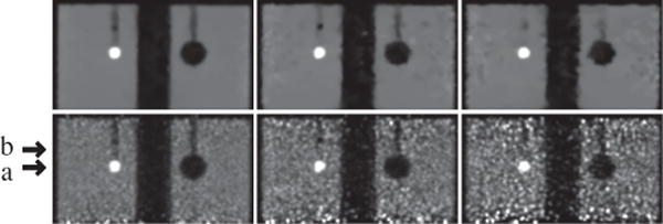
The Jaszczak phantom containing 6 sections of cold rods of diameters 4.8, 6.4, 7.9, 9.5, 11.1, and 12.7 mm is used for characterizing reconstruction spatial resolution. A set of full-count, list-mode TOF-PET data containing ∼250 million events were acquired from the phantom; low-count data sets with 63 and 25 million events (i.e., 1/4 and 1/10 of the full counts) were extracted by randomly sampling the full-count data. With each of the full- and low-count data sets, the image of the Jaszczak phantom is reconstructed on a 3D array of 128×128×82 identical cubic voxels of size 2 × 2 × 2 mm³; the standard deviation of matrix $\mathcal{G}$ is 1.0 times of the voxel size; and constraint parameter t₁ is determined by use of the scheme described in Ref. [28]. We display reconstructions within a coronal slice at x = 4 mm (plane of x = 0 mm includes the z axis) in Fig. 1, and within transverse slices at z = 22 mm and 74 mm from the axial center in Figs. 2 and 3, respectively, along with the corresponding reference images.

Figure 1.

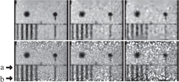
Reconstruction (row 1) and reference (row 2) images within a coronal plane of the Jaszczak phantom at x = 4 mm obtained from data of 251 (column 1), 63 (column 2), and 25 (column 3) million counts, respectively. Arrows (a) and (b) highlight the axial positions of the two transverse slices shown in Figs. 2 and 3 below. Display window: [200, 3000] a.u.

Figure 2.

Reconstruction (row 1) and reference (row 2) images within a transverse slice, indicated by arrow (a) in Fig. 1, of the Jaszczak phantom obtained from data of 251 (column 1), 63 (column 2), and 25 (column 3) million counts, respectively. Display window: [200, 3000] a.u.

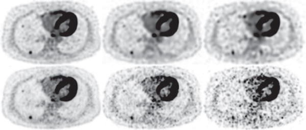
Figure 3.

Reconstruction (row 1) and reference (row 2) images within a transverse slice, indicated by arrow (b) in Fig. 1, of the Jaszczak phantom obtained from data of 251 (column 1), 63 (column 2), and 25 (column 3) million counts, respectively. Display window: [200, 3000] a.u.

2) Reconstructions from full-count data

While the middle portions in the images appear visually comparable (see column 1 in Figs. 1 and 2), it can be observed that the image-quality deterioration in the regions toward the top and bottom of the reference image appears to be reduced in the images reconstructed (see images in column 1 of Figs. 1 and 3). The images reconstructed have a reduced level of background noise compared to that of the reference image in which the cold rods especially in the section containing the rods of second to smallest diameter (see column 1 of Fig. 3) are visually less discernible than the counterparts in the former.

3) Reconstructions from low-count data

In columns 2 and 3 in Figs. 1–3, images reconstructed from the two low-count data sets, along with the corresponding reference images, are shown. As expected, image quality decreases as the photon counts are lowered. The images reconstructed show suppressed background noise relative to their reference counterparts. In particular, significant deterioration observed in the top and bottom regions of the reference image is compensated considerably for in the reconstructions obtained with the algorithm (see images in columns 2 and 3 in Figs. 1 and 3), suggesting that the algorithm proposed can yield an improved effective AVC over that of the reference images from low-count data.

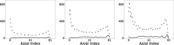
4) Axial volume coverage

We define AVC metric S_ℓ as

$${\mathrm{S}}_{\mathrm{\ell }}=\sqrt{\frac{{\displaystyle \sum _{j\in {\mathrm{\Omega }}_{\mathrm{\ell }}}{\left(u_{j_{\mathrm{\ell }}}-{\overline{u}}_{\mathrm{\ell }}\right)}^2}}{T_{\mathrm{\ell }}-1}}$$ (6)

for characterizing the reconstruction “variance” at transverse slice ℓ, where T_ℓ and Ω_ℓ denote the total number of voxels and the set of the voxel indices contained in ROIs selected within transverse slice ℓ, $u_{j_{\mathrm{\ell }}}$ is entry j_ℓ of image vector u for voxels within Ω_ℓ, and ${\overline{u}}_{\mathrm{\ell }}$ the mean-voxel value in the selected ROIs within slice ℓ. We select ROIs of rectangular shape within transverse slices ℓ in the background region. Therefore, a low, flat AVC is desired, and the height and flatness extent of AVC metric S_ℓ as a function of ℓ can be used as measures of the AVC goodness. For the images reconstructed, we compute and plot their S_ℓ as functions of ℓ in Fig. 4, along with their counterparts from the reference images. It can be observed that the S_ℓ curves of images reconstructed are flatter and lower than those of the reference images, especially toward both ends of the axial field of view (FOV), indicating reconstructions with improved AVC over the reference images.

Figure 4.

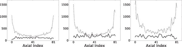
AVC metric S of the reconstruction (solid) and reference (dashed) images of the Jaszczak phantom obtained from data of 251 (column 1), 63 (column 2), and 25 (column 3) million counts, respectively.

B. Image reconstruction of the IEC phantom

1) Study materials

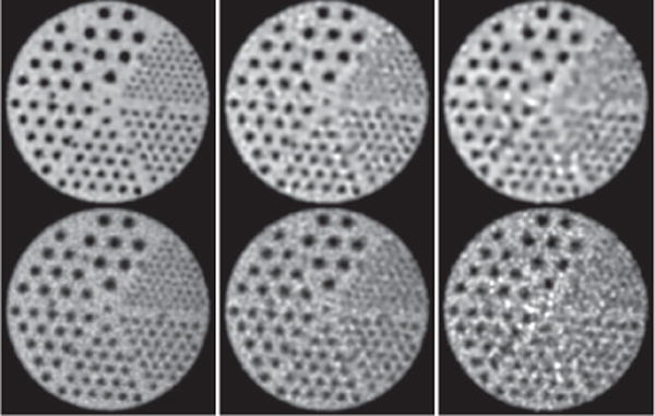
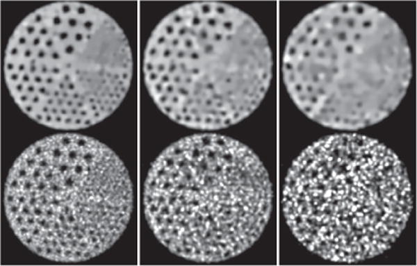
The IEC phantom embedded with 6 fillable spheres of diameters 10, 13, 17, 22, 28, and 37 mm for evaluation of reconstruction contrast (and spatial) resolution is used for collecting a set of full-count, list-mode TOF-PET data of ∼100 million counts. The two largest spheres have zero activity, while the other four are filled with positron-emitter activity at a concentration level 4 times of the background-activity level. We then extracted low-count data sets of 25 and 10 million counts (i.e., one quarter and one tenth of the full counts) by randomly sampling the full-count data set. Images of the phantom are reconstructed on a 3D array of N = 288 × 288 × 82 identical cubic voxels of size 2 × 2 × 2 mm³; the standard deviation of matrix $\mathcal{G}$ is 1.0 times of the voxel size; and constraint parameter t₁ is determined by use of the scheme described in Ref. [28].

2) Reconstructions from full-count data

In column 1 of Figs. 5–7, we display images reconstructed from the full-count data set, along with the reference images. It can be observed that the reconstructions are with visually enhanced contrast (and spatial) resolution and considerably reduced background noise over the reference images. Enhanced background uniformity is somewhat expected of a regularized reconstruction with most forms of regularization, but the simultaneous enhancement in contrast and spatial resolution is not. Again, the algorithm proposed appears to yield images with visually comparable quality throughout the longitudinal FOV, whereas the reference images show considerable quality deterioration in its top and bottom region (see column 1 in Fig. 5 and 7). The observation is consistent with that of the Jaszczak-phantom results, suggesting that the algorithm proposed yields an improved, effective AVC over that of the reference image from full-count data.

Figure 5.

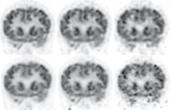
Reconstruction (row 1) and reference (row 2) images within a coronal slice of the IEC phantom obtained from data of 100 (column 1), 25 (column 2), and 10 (column 3) million counts, respectively. Arrows (a) and (b) highlight the axial positions of the two transverse slices shown in Figs. 6 and 7 below. Display window: [0, 1800] a.u.

Figure 7.

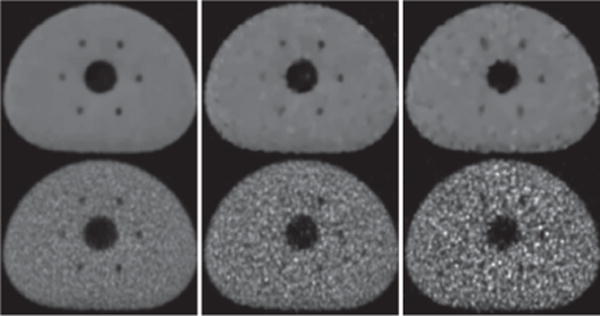
Reconstruction (row 1) and reference (row 2) images within a transverse slice, indicated by arrow (b) in Fig. 5, of the IEC phantom obtained from data of 100 (column 1), 25 (column 2), and 10 (column 3) million counts, respectively. Display window: [0, 1800] a.u.

3) Reconstructions from low-count data

We also display in columns 2 and 3 in Figs. 5–7 images within a coronal and two transverse slices reconstructed by use of the algorithm, along with the corresponding reference images, from the two low-count data sets of the IEC phantom. Similar to the Jaszczak-phantom study, while the overall image quality diminishes as the photon counts are lowered, the contrast levels of hot and cold spheres appear to be retained, with the background noise in the reconstructions effectively suppressed relative to those of the reference images. Also, no significant quality deterioration similar to those observed in the top and bottom regions of the reference images is observed in the reconstructions (see columns 2 and 3 in Figs. 5 and 7), indicating that the algorithm proposed can improve the effective AVC over that of the reference image from low-count data.

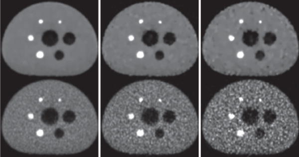
4) Analysis of reconstruction contrast

We calculate NEMA-contrast metrics Q_H,r or Q_C,r for sphere r of the 4 hot spheres or of the 2 cold spheres. Also, 6 regions-of-interest (ROIs) are selected for computation of the background-noise metric N_p within ROI p. We display in Fig. 8 the NEMA metrics computed for full- and low-count data. The quantitative results in rows 1–3 of Fig. 8 show that the algorithm proposed yield reconstructions with consistent contrast levels of hot and cold spheres, and level of background noise, for full- and low-count data sets. For the low-count data, while an increased level of background noise is observed in the reconstructions and in the reference images, the level of background noise in the former is lower than that in the latter. The contrast levels of the hot spheres in the reference images from the low-count data (see rows 2 & 3 and column 1 of Fig. 8) appear “higher” than that in the reference image from the full-count data (see row 1 and column 1 of Fig. 8). The false improvement results from the higher noise in the reference reconstruction from low-count data.

Figure 8.

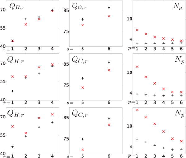
NEMA-contrast metrics Q_H,r for hot spheres 1–4 (column 1) and Q_C,r for cold spheres 5–6 (column 2) and NEMA-background-variability metric N_p (column 3) computed from the reconstruction (+) and reference (×) images of the IEC phantom for data of 100 (row 1), 25 (row 2), and 10 (row 3) million counts, respectively.

5) Axial volume coverage

Using Eq. (6), we calculate AVC metric S_ℓ from the reconstructed and reference images, and plot them in Fig. 9. It can be observed in Fig. 9 that AVC metrics S_ℓ of the reconstruction images are generally flatter and lower than those of the reference images, especially toward both ends of the axial FOV, indicating that the algorithm proposed can yield reconstructions with improved AVC over the reference images.

Figure 9.

AVC metric S_ℓ of the reconstruction (solid) and reference (dashed) images of the IEC phantom obtained from data of 100 (column 1), 25 (column 2), and 10 (column 3) million counts, respectively.

C. Image reconstruction of the human subject

1) Study materials

In the human-subject study, data were acquired sequentially at 5 consecutive, but partially overlapping, patient-bed positions for covering the head, neck, and torso of the subject. For each bed position, we reconstruct an image on a 3D array of N = 288 × 288 × 82 identical cubic voxels of size 2 mm, with its short dimensionplaced in parallel to the central axis, and its center coinciding with the center point of axial FOV, of the scanner. There is a separation of 100 mm between the centers of two consecutive bed positions along the central axis of the scanner. Considering the physical, longitudinal length (∼ 164 mm) of the scanner, the 100-mm separation thus results in ∼ 39% overlap of each pair of consecutive bed positions. The purpose of the bed-position overlap is designed to compensate for the deterioration of image quality in regions toward both ends of a bed position when the images from all of the overlapping bed positions are assembled to form an upper-body image of the subjects.

The 5 data sets, referred to as the full-count data sets, collected at the 5 bed positions contain approximately 80, 60, 52, 54, and 56 million total counts, with scatter and random events corrected for. Furthermore, from each of the full-count data sets, we randomly extract two data sets containing one-quarter and one-tenth of the total counts to mimic low-count data sets. From the full- or low-count data sets collected at a bed position, we reconstruct images with the standard deviation in matrix $\mathcal{G}$ chosen as 1.0, 1.2, and 1.5 times of the voxel size for full-count data and for the low-count data sets containing one-quarter and one-tenth of the full-count data.

2) Image reconstruction of the head/neck region

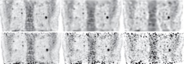
We first reconstructed from full-count data collected at bed-position 1 covering the head and upper portion of the neck of the human subject, and show in column 1 of Figs. 10 and 11 images within sagittal and coronal slices, and in column 1 of Fig. 12 images within the transverse slice indicated in Fig. 10, along with the corresponding reference images. It can be observed that reconstructions visually appear to be of slightly improved spatial and contrast resolution over, yet with a background-noise level comparable to, that of the reference images. We also carried out reconstructions from the low-count data sets and show in columns 2 and 3 of Figs. 10–12 images within the same sagittal, coronal, and transverse slices as those in the full-count reconstructions. While low-count-data reconstructions are, as expected, with reduced image quality as compared to their corresponding full-count-data reconstructions, they appear to have an improved level of spatial and contrast resolution yet with slightly reduced background noise over their reference counterparts. Moreover, the reconstruction from one-quarter of the full-count data appears to have spatial/contrast resolution better than, and a noise level comparable to, the full-count reference images. Overall, the AVCs in reconstructed images for all of the data sets remain unchanged, while an increased noise and some false hot spots can be observed in the regions toward to the bottom portions of the reference images in Figs. 10 and 11, suggesting that the algorithm proposed yields an improved AVC for full- and low-count data sets.

Figure 10.

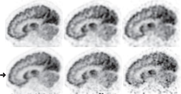
Reconstruction (row 1) and reference(row 2) images within a sagittal slice of the head/neck of the human subject obtained from data of 80 (column 1), 20 (column 2), and 8 (column 3) million counts, respectively. The arrow highlights the axial position of the transverse slice within which the image is shown in Fig. 12 below. Display window: [−1625, 0] a.u.

Figure 11.

Reconstruction (row 1) and reference (row 2) images within a coronal slice of the head/neck of the human subject obtained from data of 80 (column 1), 20 (column 2), and 8 (column 3) million counts, respectively. Display window: [−1625, 0] a.u.

Figure 12.

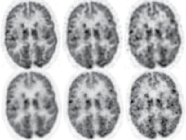
Reconstruction (row 1) and reference (row 2) images within a transverse slice, indicated by the arrow in Fig. 10 obtained from data of 80 (column 1), 20 (column 2), and 8 (column 3) million counts, respectively. Display window: [−1625, 0] a.u.

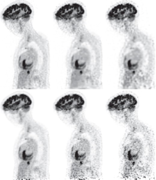
3) Image reconstruction of the torso region

We also conducted reconstructions from full- and low-count data collected at bed-position 4 covering the torso region containing the lung of the human subject, and show in Figs. 13–15 images within sagittal, coronal, and transverse slices, along with their respective reference images. Again, in terms of spatial and contrast resolution and background noise, observations similar to those for bed-position 1 covering the head and neck can be made for the reconstructions covering the torso region. When the data-count level deceases substantially, the spatial and contrast resolution in the reconstructions diminishes, as expected, but at a pace slower than that in the reference images, as the low-count-data reference images display considerably heightened noise levels. In particular, significant amount of false hot spots can be descried especially in the top and bottom regions in the reference images in Figs. 13 and 14 for full- and low-count data. It is the need to compensate for the considerable deterioration of image quality observed in the regions toward both ends of the axial FOV in the reference images that motivates the current clinical scanning protocol of data collection at multiple, overlapping bed positions.

Figure 13.

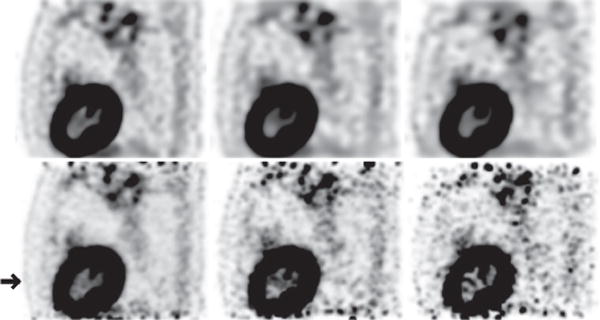
Reconstruction (row 1) and reference (row 2) images within a sagittal slice of the torso of the human subject obtained from data of 54 (column 1), 13.5 (column 2), and 5.4 (column 3) million counts, respectively. The arrow highlights the axial position of the transverse slice within which the image is shown in Fig. 15 below. Display window: [−300, 0] a.u.

Figure 15.

Reconstruction (row 1) and reference (row 2) images within a transverse slice, indicated by the arrow in Fig. 13 obtained from data of 54 (column 1), 13.5 (column 2), and 5.4 (column 3) million counts, respectively. Display window: [−300, 0] a.u.

Figure 14.

Reconstruction (row 1) and reference (row 2) images within a coronal slice of the torso of the human subject obtained from data of 54 (column 1), 13.5 (column 2), and 5.4 (column 3) million counts, respectively. Display window: [−300, 0] a.u.

4) Image reconstructions of the upper-body

We finally reconstructed images from data of the full- or a low-count level collected at the five overlapping bed positions and form an upper-body reconstruction of the subject by concatenating the five reconstructions according to the five bed positions. As mentioned above, the axial overlap between two adjacent bed positions is about 64 mm amounting to 39% of the axial FOV of one single bed position. In Figs. 16 and 17, we display the images within coronal and sagittal slices of the upper-body reconstruction for the human subject for full- and low-count data sets. The 39% bed-position-overlap effectively eliminates much of the false hot spots observed in reference images of the head/neck and torso obtained from single bed-position data, which, however, is done at the cost of a significantly reduced efficiency in terms of total AVC and/or imaging time. On the other hand, observations made above for reconstructions obtained in a single bed-position scan remain unchanged. While their quality diminishes as the level of data counts decreases, the reconstructions appear to maintain an improvement over their reference images in terms of spatial and contrast resolution as well as background noise. In particular, as shown in Figs. 16 and 17, false hot spots can be observed in the region toward the bottom of the axial FOV in the reference images, including those obtained from the full-count data, due to the fact that there is no overlap scanning for the region. Conversely, it can be seen that the reconstructions for full- and low-count data appear to be free of such false hot spots observed in the reference images.

Figure 16.

Reconstruction (row 1) and reference (row 2) images within a sagittal slice of the upper body of the human subject obtained from data of 302 (column 1), 75.5 (column 2), and 30.2 (column 3) million counts, respectively, collected at the 5 overlapping bed positions. Display window: [−1200, 0] a.u.

Figure 17.

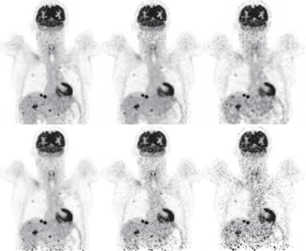
Reconstruction (row 1) and reference (row 2) images within a coronal slice of the upper body of the human subject obtained from the full- and low-count data sets of 302 (column 1), 75.5 (column 2), and 30.2 (column 3) million counts, respectively, collected at the 5 overlapping bed positions. Display window: [−1200, 0] a.u.

V. DISCUSSIONS

We have investigated an optimization-based image reconstruction from list-mode data collected with SiPM-based digital TOF PET, in which the image is designed as a solution to a convex, but non-smooth, optimization program containing a KL-data divergence and image-TV constraint, and a CP algorithm is proposed to reconstruct the image through solving the optimization program. When applied to full-count data, the algorithm appears to yield reconstructions with visualization, spatial resolution, and NEMA contrast metrics comparable to, and an AVC larger than, that of the reference images. Furthermore, we explore and demonstrate the algorithm’s potential for image reconstruction from low-count data, mimicking low-dose and/or fast imaging conditions of practical interest. Results of visual inspection and quantitative-metric analysis reveal that the algorithm proposed can reconstruct images with enhanced spatial and contrast resolution, suppressed background noise, and increased AVC over the reference images from list-mode TOF-PET data of low-count levels.

As the focus of the work is to achieve the convergent reconstruction (i.e., the designed solution to the optimization program,) the algorithm takes a considerable number (~2000) of iterations until achieving the convergent reconstruction, thus minimizing the impact of iterations on the reconstruction. However, it is also of interest to inspect reconstructions at earlier iterations for gaining insights that may be useful for the design of practical reconstruction procedures involving only a small number of iterations for yielding images comparable to the reference or the convergent reconstruction. In Fig. 18, we display reconstructions of intermediate iterations from data of the human subject collected at bed-position 4. It can be observed that, despite some visual texture difference, reconstructions at earlier iterations appear to reveal leading features of interest such as hot spots and spine disks observed in the convergent reconstruction. Similar observation can be made for reconstructions of the physical phantoms and human subject at other bed positions.

Figure 18.

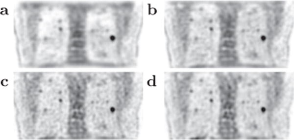
Reconstructions at iterations 30 (a), 50 (b), and 150 (c), along with the convergent reconstruction (d) within a coronal slice of the human subject. Display window: [−300, 0] a.u.

We remind that, while the study is to demonstrate that the algorithm can be a useful tool for exploring, and for yielding insights into, the design of practical optimization-based reconstruction in TOF-PET imaging, it is not intended to establish and assess the truly application-specific utility of the reconstruction design and algorithm proposed, especially as a practical image-reconstruction tool for use in routine or clinical TOF-PET applications, because such an assessment must be clinical/preclinical task-specific and must consider adequately imaging-protocol-specific conditions, which are neither defined nor considered in the work.

While the KL-data divergence was considered in the work, it is of theoretical and practical significance to investigate optimization-based reconstruction employing other data divergences. Optimization programs with non-KL-data divergences and their associated CP algorithms can readily be developed mathematically. However, numerous data divergences with forms (e.g., ℓ₂ or ℓ₁-form [28], [32]) of interest can be written only in a form in which the number of computation operations involved is in the order of ∼ 10¹⁵, i.e., the product of the total numbers of TOF bins and the number of image voxels. For an advanced, clinical TOF-PET scanner, this can be a huge number and can thus impose a practically prohibitively high demand (at least currently) on computational memory and time. There is also increased interest in exploring TOF-PET scanning configurations with sparsely populated detector modules for reducing hardware cost and complexity [28]. The optimization program and algorithm developed in the work can readily be extended to exploring image reconstruction from list-mode data collected with TOF-PET scanning configurations populated only sparsely by detector modules.

VI. CONCLUSION

We have developed an optimization-based approach for image reconstruction from list-mode data collected in advanced TOF PET and exploited the approach to investigating image reconstructions from TOF-PET data of different count levels collected from both physical phantom and human subject studies. The results suggest that an appropriately designed optimization-based reconstruction approach can yield TOF-PET images with enhanced spatial and contrast resolution, suppressed background noise, and increased AVC, over those obtained with a standard clinical reconstruction algorithm. The optimization-based reconstruction approach can be exploited for yielding insights into potential quality-upper bound of reconstructed images in, and design of scanning protocols of, TOF-PET imaging of practical significance.

Figure 6.

Reconstruction (row 1) and reference (row 2) images within a transverse slice, indicated by arrow (a) in Fig. 5, of the IEC phantom obtained from data of 100 (column 1), 25 (column 2), and 10 (column 3) million counts, respectively. Display window: [0, 1800] a.u.

APPENDIX: DERIVATION OF THE CP ALGORITHM

To derive the instance of the CP algorithm for Eq. (4), we reformulate it as [25], [28]

$$\mathbf{u}\ast =\underset{\mathbf{u}}{\arg min}\{\mathrm{\lambda }({\displaystyle \sum _k{[\mathrm{ℛ}\mathbf{u}]}_k-{\displaystyle \sum _i\ln {[\mathrm{\mathscr{H}}\mathbf{u}+c^{\prime }]}_{k_i{\tau }_i}}})\}+{\delta }_{\text{Diamond(}\nu t_1\text{)}}\left({\left|\nu \nabla \mathbf{f}\right|}_{\text{MAG}}\right)+{\delta }_P(\mathbf{f})\},$$ (7)

where λ and ν are positive parameters, ∇ represents a gradient matrix of size 3N × N with its transpose given by ${\nabla }^{\top }=({\nabla }_x^{\top },{\nabla }_y^{\top },{\nabla }_z^{\top })$; superscript ‘⊤’ indicates a transpose operation; ${\nabla }_x^{\top }$, ${\nabla }_y^{\top }$, and ${\nabla }_z^{\top }$ are matrices of size N × N representing two-point differences along x-, y-, and z-axis, respectively, yielding vectors ${\nabla }_x^{\top }$, ${\nabla }_y^{\top }$, and ${\nabla }_z^{\top }$ of size N, which in turn form vector ∇f of size 3N in a concatenated form in the order of x, y, and z; |∇f|_MAG denotes a vector of size N in which entry j is given by ${(|\nabla \mathbf{f}{|}_{\text{MAG}})}_j=\sqrt{{(\nabla \mathbf{f})}_j^2+{(\nabla \mathbf{f})}_{j+N}^2+{(\nabla \mathbf{f})}_{j+2N}^2}$; and indicator functions δ_P (x) and ${\delta }_{\text{Diamond}(\nu t_1)}(\mathbf{x})$ are defined as:

$$\begin{array}{l}{\delta }_P(\mathbf{x})\equiv \{\begin{array}{ll}0\hfill & \mathbf{x}\ge 0\hfill \\ \mathrm{\infty }\hfill & \text{Otherwise}\hfill \end{array}\\ {\delta }_{\text{Diamond}(\nu t_1)}(\mathbf{x})\equiv \{\begin{array}{ll}0\hfill & {\Vert \mathbf{x}\Vert }_1\le \nu t_1\hfill \\ \mathrm{\infty }\hfill & {\Vert \mathbf{x}\Vert }_1>\nu t_1\hfill \end{array}.\end{array}$$ (8)

We consider two vectors a and b of sizes kN and N, with entries a_j and b_j, where k ≥ 1 is a positive integer, and define vectors ab and a/b of sizes kN as the multiplication and division of a and b, with entry j given by ${(\mathbf{a}\mathbf{b})}_j=a_j{b}_{j_m}$ and ${(\mathbf{a}/\mathbf{b})}_j=a_j{b}_{j_m}$, respectively, where j = 1, 2, …, kN, and j_m = mod(j, N) indicates the remainder of j dividing by N, and $b_{j_m}\ne 0$. When k = 1, a^⊤b denotes their inner product of a and b.

The generic CP algorithm solves simultaneously a primal minimization and dual maximization problems below:

$${\mathbf{x}}^{\ast }=\underset{\mathbf{x}}{\arg min}\{F(K\mathbf{x})+G(\mathbf{x})\},$$ (9)

$${\mathbf{y}}^{\ast }=\underset{\mathbf{y}}{\arg max}\{-F^{\ast }(\mathbf{y})-G^{\ast }(-K^{\top }\mathbf{y})\},$$ (10)

where primal and dual variables x and y are vectors in spaces X and Y, K a linear transform from X to Y, F and G convex functions mapping the X and Y spaces to non-negative real numbers, and the convex conjugate functions

$$\begin{array}{l}{F}^{\ast }(\mathbf{y})=\underset{y^{\prime }}{\text{max}}\{{\mathbf{y}}^{\top }{y}^{\prime }-F(y^{\prime })\}\\ G^{\ast }(\mathbf{y})=\underset{y^{\prime }}{\text{max}}\{{\mathbf{y}}^{\top }{y}^{\prime }-G(y^{\prime })\}.\end{array}$$ (11)

The pseudo-codes of the generic CP algorithm that solves the primal-dual problem in Eqs. (9) and (10) are given in Algorithm 2, in which the proximal mappings are given by

$$\mathit{pro}{x}_{\sigma }[F^{\ast }](\mathbf{y})=\underset{y^{\prime }}{\arg min}\left\{F^{\ast }(y^{\prime })+\frac{1}{2}{(\mathbf{y}-y^{\prime })}^{\top }\left(\frac{\mathbf{y}-y^{\prime }}{\sigma }\right)\right\}$$ (12)

$$\mathit{pro}{x}_{\tau }[G](\mathbf{x})=\underset{x^{\prime }}{\arg min}\left\{G(x^{\prime })+\frac{1}{2}{(\mathbf{x}-x^{\prime })}^{\top }\left(\frac{\mathbf{x}-x^{\prime }}{\tau }\right)\right\}.$$ (13)

Algorithm 2.

Pseudo codes of the generic CP algorithm

1: L ← ||K||SV, τ ← 1/L, σ ← 1/L

2: θ ← 1; n ← 0

3: initialize x0 and y0 to zero

4: ${\overline{x}}_0\leftarrow {\mathbf{x}}_0$

5: repeat

6: ${\mathbf{y}}_{n+1}\leftarrow \mathit{pro}{x}_{\sigma }[F^{\ast }]({\mathbf{y}}_n+\sigma K{\overline{x}}_n)$

7: xn+1 ← proxτ[G](xn − τK⊤yn+1)

8: ${\overline{x}}_{n+1}\leftarrow {\mathbf{x}}_{n+1}+\theta ({\mathbf{x}}_{n+1}-{\mathbf{x}}_n)$

9: n ← n + 1

10: : until $n\ge \mathcal{N}$

11: OUTPUT: image ${\mathbf{x}}_{\mathcal{N}}$

We show below that Eq. (7) can be interpreted as a primal problem. Letting

$$\begin{array}{l}\mathbf{x}=\mathbf{f},\mathbf{r}=\mathrm{ℛ}\mathcal{G}\mathbf{f},\mathbf{v}=\mathrm{\mathscr{H}}\mathcal{G}\mathbf{f},\\ \mathbf{z}=\nu \nabla \mathbf{f},K^{\top }=({\mathcal{G}}^{\top }{\mathrm{ℛ}}^{\top },{\mathcal{G}}^{\top }{\mathrm{\mathscr{H}}}^{\top },\nu {\nabla }^{\top }),\end{array}$$ (14)

we can rewrite Eq. (7) as

$${\mathbf{u}}^{\ast }=\mathcal{G}\underset{\mathbf{f}}{\arg min}\{F(\mathbf{r},\mathbf{v},\mathbf{z})+G(\mathbf{f})\},$$ (15)

where F(r, v, z) = F₁(r) + F₂(v) + F₃(z),

$$F_1(\mathbf{r})=\mathrm{\lambda }{\displaystyle \sum _k{[\mathbf{r}]}_k},$$ (16)

$$F_2(\mathbf{v})=-\mathrm{\lambda }{\displaystyle \sum _i\log {[\mathbf{v}+c^{\prime }]}_{k_i{\tau }_i}},$$ (17)

$$F_3(\mathbf{z})={\delta }_{\text{Diamond}(\nu t_1)}\left({\Vert \mathbf{z}\Vert }_{\text{MAG}}\right),$$ (18)

$$G(\mathbf{x})={\delta }_P(\mathbf{x}),$$ (19)

||z||_MAG a vector of size N with entry j given by ${\left({\Vert \mathbf{z}\Vert }_{\text{MAG}}\right)}_j=\sqrt{{|{(\mathbf{z})}_j|}^2+{|{(\mathbf{z})}_{j+N}|}^2+{|{(\mathbf{z})}_{j+2N}|}^2}$, and (z)_j entry j of vector z. Thus, the optimization program in Eq. (7) is cast into a primal minimization problem in Eq. (15).

The convex conjugates of F and G are obtained as

$$\begin{gathered} F^{\ast }(\mathbf{w},\mathbf{p},\mathbf{q})=F_1^{\ast }(\mathbf{w})+F_2^{\ast }(\mathbf{p})+F_3^{\ast }(\mathbf{q}) \\ {G}^{\ast }(\mathbf{y})=\underset{\mathbf{x}}{\text{max}}\{{\mathbf{y}}^{\top }\mathbf{x}-G(\mathbf{x})\}={\delta }_P(-\mathbf{y}), \end{gathered}$$ (20)

where vectors w, p, and q are of sizes M_R, M_E, and 3N,

$$F_1^{\ast }(\mathbf{w})=\underset{\mathbf{r}}{\text{max}}\{{\mathbf{w}}^{\top }\mathbf{r}-F_1(\mathbf{r})\}=\mathrm{\lambda }\delta (\mathbf{w}-{\mathbf{\lambda }}_R),$$ (21)

$$F_2^{\ast }(\mathbf{p})=\underset{\mathbf{v}}{\text{max}}\{{\mathbf{p}}^{\top }\mathbf{v}-F_2(\mathbf{v})\}=-{c^{\prime }}^{\top }\mathbf{p}+{\displaystyle \sum _i{[-{\mathbf{\lambda }}_E+\mathrm{\lambda }\log (-\frac{{\mathbf{\lambda }}_E}{\mathbf{p}})]}_{k_i{\tau }_i}}\mathrm{s}.\mathrm{t}.{(\mathbf{p})}_{k_i{\tau }_i}<0,$$ (22)

$$F_3^{\ast }(\mathbf{q})=\underset{\mathbf{z}}{\text{max}}\{{\mathbf{q}}^{\top }\mathbf{z}-F_3(\mathbf{z})\}=\nu t_1{\Vert \left({\Vert \mathbf{q}\Vert }_{\text{MAG}}\right)\Vert }_{\mathrm{\infty }},$$ (23)

vectors λ_R of size M_R and λ_E of size M_E with constant entries λ, ${(\mathbf{p})}_{k_i{\tau }_i}$ the entry of vector p in TOF bin τ_i along LOR k_i, || · ||_∞ norm the largest entry of a vector, ||q||_MAG a vector of size N with entry j given by ${\left({\Vert \mathbf{q}\Vert }_{\text{MAG}}\right)}_j=\sqrt{{|{(\mathbf{q})}_j|}^2+{|{(\mathbf{q})}_{j+N}|}^2+{|{(\mathbf{q})}_{j+2N}|}^2}$, and (q)_j entry j of vector q Using Eqs. (20)–(23) in Eq. (10), we obtain the dual maximization problem as

$$({\mathbf{w}}^{\ast },{\mathbf{p}}^{\ast },{\mathbf{q}}^{\ast })=\underset{\mathbf{w},\mathbf{p},\mathbf{q}}{\arg max}\{-\mathrm{\lambda }\delta (\mathbf{w}-{\mathbf{\lambda }}_R)+{c^{\prime }}^{\top }\mathbf{p}-{\displaystyle \sum _i}{[-{\mathbf{\lambda }}_E+\mathrm{\lambda }\log (-\frac{{\mathbf{\lambda }}_E}{\mathbf{p}})]}_{k_i{\tau }_i}-\nu t_1{\Vert ({\Vert \mathbf{q}\Vert }_{\text{MAG}})\Vert }_{\mathrm{\infty }}-{\delta }_P(-{\mathcal{G}}^{\top }{\mathrm{ℛ}}^{\top }\mathbf{w}-{\mathcal{G}}^{\top }{\mathrm{\mathscr{H}}}^{\top }\mathbf{p}-\nu {\nabla }^{\top }\mathbf{q})\}.$$ (24)

Also, using Eqs. (20)–(23) in Eqs. (12) and (13), we obtain the proximal mappings, which are the key steps of the CP algorithm of our interest, as

$$\mathit{pro}{x}_{\sigma }[F_1^{\ast }](\mathbf{w})={\mathbf{\lambda }}_R,$$ (25)

$$\mathit{pro}{x}_{\sigma }[F_2^{\ast }](\mathbf{p})=\frac{1}{2}\left(\mathbf{p}+\sigma c^{\prime }-\sqrt{{(\mathbf{p}+\sigma c^{\prime })}^2+4\sigma {\mathbf{\lambda }}_E}\right),$$ (26)

$$\mathit{pro}{x}_{\sigma }[F_3^{\ast }](\mathbf{q})=\mathbf{q}-\sigma \mathbf{q}\mathbf{P}\mathbf{r}\mathbf{o}\mathbf{j}\mathbf{e}\mathbf{c}\mathbf{t}\mathbf{O}\mathbf{n}\mathbf{t}\mathbf{o}{\mathrm{\ell }}_1\mathbf{B}\mathbf{a}\mathbf{l}{\mathbf{l}}_{\nu t_1}({\Vert \mathbf{q}\Vert }_{\text{MAG}}/\sigma )/{\Vert \mathbf{q}\Vert }_{\text{MAG}},$$ (27)

$$\mathit{pro}{x}_{\tau }[G](\mathbf{f})=\text{pos}(\mathbf{f}),$$ (28)

where $\mathbf{P}\mathbf{r}\mathbf{o}\mathbf{j}\mathbf{e}\mathbf{c}\mathbf{t}\mathbf{O}\mathbf{n}\mathbf{t}\mathbf{o}{\mathrm{\ell }}_1\mathbf{B}\mathbf{a}\mathbf{l}{\mathbf{l}}_{\nu t_1}(x^{\prime })$ yields a vector of size N by projecting vector x′ of size N onto the ℓ₁-ball of scale νt₁, and pos(f) = 0 and f_i for f_i ≤ 0 and f_i > 0, respectively, enforcing the non-negativity constraint.

Using $\mathit{pro}{x}_{\sigma }[F_1^{\ast }](\mathbf{w})$, $\mathit{pro}{x}_{\sigma }[F_2^{\ast }](\mathbf{p})$, and $\mathit{pro}{x}_{\sigma }[F_3^{\ast }](\mathbf{q})$ in Eqs. (25), (26) and (27) to replace prox_σ[F^∗](y) in Line 6, and prox_τ[G](f) in Eq. (28) to substitute prox_τ[G](x) in Line 7, in Algorithm 2, we obtain the pseudo codes in Lines 6 and 7 of Algorithm 1 for the CP-algorithm instance for solving Eq. (4), or equivalently, the program in Eq. (15).

References

- 1.Snyder DL, Politte D. Image reconstruction from list-mode data in an emission tomography system having time-of-flight measurements. IEEE Trans Nucl Sci. 1983;30(3):1843–1849. [Google Scholar]
- 2.Chen C-T, Metz CE. A simplified EM reconstruction algorithm for TOFPET. IEEE Trans Nucl Sci. 1985;32(1):885–888. [Google Scholar]
- 3.Barrett HH, et al. List-mode likelihood. J Opt Soc Amer. 1997;14(11):2914–2923. doi: 10.1364/josaa.14.002914. [DOI] [PMC free article] [PubMed] [Google Scholar]
- 4.Reader AJ, et al. One-pass list-mode EM algorithm for high-resolution 3-D PET image reconstruction into large arrays. IEEE Trans Nucl Sci. 2002;49(3):693–699. [Google Scholar]
- 5.Pratx G, et al. Fast list-mode reconstruction for time-of-flight PET using graphics hardware. IEEE Trans Nucl Sci. 2011;58(1):105–109. [Google Scholar]
- 6.Wang W, Gindi G. Noise analysis of MAP-EM algorithms for emission tomography. Phys Med Biol. 1997;42:2215–2232. doi: 10.1088/0031-9155/42/11/015. [DOI] [PubMed] [Google Scholar]
- 7.Qi J, Leahy RM. A theoretical study of the contrast recovery and variance of MAP reconstructions from PET data. IEEE Trans Med Imag. 1999;18(4):293–305. doi: 10.1109/42.768839. [DOI] [PubMed] [Google Scholar]
- 8.Nuyts J, et al. A concave prior penalizing relative differences for maximum-a-posteriori reconstruction in emission tomography. IEEE Trans Nucl Sci. 2002;49(1):56–60. [Google Scholar]
- 9.Bai B, et al. MAP reconstruction for Fourier rebinned TOF-PET data. Phys Med Biol. 2014;59(4):925. doi: 10.1088/0031-9155/59/4/925. [DOI] [PMC free article] [PubMed] [Google Scholar]
- 10.Kaufman L. Maximum likelihood, least squares, and penalized least squares for pet. IEEE Trans Med Imag. 1993;12(2):200–214. doi: 10.1109/42.232249. [DOI] [PubMed] [Google Scholar]
- 11.Mumcuoğlu EÜ, et al. Bayesian reconstruction of PET images: methodology and performance analysis. Phys Med Biol. 1996;41(9):1777. doi: 10.1088/0031-9155/41/9/015. [DOI] [PubMed] [Google Scholar]
- 12.Fessler J, Rogers WL. Spatial resolution properties of penalized-likelihood image reconstruction: space-invariant tomographs. IEEE Trans Imag Proc. 1996;5(9):1346–1358. doi: 10.1109/83.535846. [DOI] [PubMed] [Google Scholar]
- 13.Hudson HM, Larkin RS. Accelerated image reconstruction using ordered subsets of projection data. IEEE Trans Med Imag. 1994;13(4):601–609. doi: 10.1109/42.363108. [DOI] [PubMed] [Google Scholar]
- 14.Liu X, et al. Comparison of 3-D reconstruction with 3D-OSEM and with FORE+ OSEM for PET. IEEE Trans Med Imag. 2001;20(8):804–814. doi: 10.1109/42.938248. [DOI] [PubMed] [Google Scholar]
- 15.Matej S, et al. Efficient 3-D TOF PET reconstruction using view-grouped histo-images: DIRECT-direct image reconstruction for TOF. IEEE Trans Med Imag. 2009;28(5):739–751. doi: 10.1109/TMI.2008.2012034. [DOI] [PMC free article] [PubMed] [Google Scholar]
- 16.Mehranian A, et al. An ordered-subsets proximal preconditioned gradient algorithm for edge-preserving PET image reconstruction. Med Phys. 2013;40(5):052503. doi: 10.1118/1.4801898. [DOI] [PubMed] [Google Scholar]
- 17.Zhou J, Qi J. Efficient fully 3D list-mode TOF PET image reconstruction using a factorized system matrix with an image domain resolution model. Phys Med Biol. 2014;59(3):541. doi: 10.1088/0031-9155/59/3/541. [DOI] [PMC free article] [PubMed] [Google Scholar]
- 18.Kim K, et al. TOF-PET ordered subset reconstruction using nonuniform separable quadratic surrogates algorithm. IEEE 11th Intern Symp Biomed Imag. 2014:963–966. [Google Scholar]
- 19.Moses WW. Recent advances and future advances in time-of-flight PET. Nucl Instr Meth Phy Resch. 2007;580(2):919–924. doi: 10.1016/j.nima.2007.06.038. [DOI] [PMC free article] [PubMed] [Google Scholar]
- 20.Lois C, et al. An assessment of the impact of incorporating time-of-flight information into clinical PET/CT imaging. J Nucl Med. 2010;51(2):237–245. doi: 10.2967/jnumed.109.068098. [DOI] [PMC free article] [PubMed] [Google Scholar]
- 21.Surti S, et al. Impact of time-of-flight PET on whole-body oncologic studies: a human observer lesion detection and localization study. J Nucl Med. 2011;52(5):712–719. doi: 10.2967/jnumed.110.086678. [DOI] [PMC free article] [PubMed] [Google Scholar]
- 22.Lewellen T, et al. Investigation of the performance of the General Electric ADVANCE positron emission tomograph in 3D mode. IEEE Trans Nucl Sci. 1996;43(4):2199–2206. [Google Scholar]
- 23.Pajevic S, et al. Noise characteristics of 3-D and 2-D PET images. IEEE Trans Med Imag. 1998;17(1):9–23. doi: 10.1109/42.668691. [DOI] [PubMed] [Google Scholar]
- 24.Chambolle A, Pock T. A first-order primal-dual algorithm for convex problems with applications to imaging. J Math Imag Vis. 2011;40:1–26. [Google Scholar]
- 25.Sidky EY, et al. Convex optimization problem prototyping for image reconstruction in computed tomography with the Chambolle–Pock algorithm. Phys Med Biol. 2012;57(10):3065–3091. doi: 10.1088/0031-9155/57/10/3065. [DOI] [PMC free article] [PubMed] [Google Scholar]
- 26.Wolf PA, et al. Few-view single photon emission computed tomography (SPECT) reconstruction based on a blurred piecewise constant object model. Phys Med Biol. 2013;58(16):5629–5652. doi: 10.1088/0031-9155/58/16/5629. [DOI] [PMC free article] [PubMed] [Google Scholar]
- 27.Sidky EY, et al. Analysis of iterative region-of-interest image reconstruction for X-ray computed tomography. J Med Imag. 2014;1(3):031007–031007. doi: 10.1117/1.JMI.1.3.031007. [DOI] [PMC free article] [PubMed] [Google Scholar]
- 28.Zhang Z, et al. Investigation of optimization-based reconstruction with an image-total-variation constraint in PET. Phys Med Biol. 2016;61(16):6055–6084. doi: 10.1088/0031-9155/61/16/6055. [DOI] [PMC free article] [PubMed] [Google Scholar]
- 29.Miller M, et al. Characterization of the vereos digital photon counting PET system. J Nucl Med. 2015;56(supplement 3):434–434. [Google Scholar]
- 30.Watson CC, et al. A single scatter simulation technique for scatter correction in 3D PET. Proc 3rd Inter Meet Ful 3D Imag Recon Radio Nucl Med Springer. 1996:255–268. [Google Scholar]
- 31.Badawi R, et al. Randoms variance reduction in 3D PET. Phys Med Biol. 1999;44(4):941–954. doi: 10.1088/0031-9155/44/4/010. [DOI] [PubMed] [Google Scholar]
- 32.Zhang Z, et al. Artifact reduction in short-scan CBCT by use of optimization-based reconstruction. Phys Med Biol. 2016;61(9):3387–3406. doi: 10.1088/0031-9155/61/9/3387. [DOI] [PMC free article] [PubMed] [Google Scholar]
- 33.Xia D, et al. Optimization-based image reconstruction with artifact reduction in C-arm CBCT. Phys Med Biol. 2016;61(20):7300–7333. doi: 10.1088/0031-9155/61/20/7300. [DOI] [PMC free article] [PubMed] [Google Scholar]