Phylogenetic Factor Analysis

Abstract

Phylogenetic comparative methods explore the relationships between quantitative traits adjusting for shared evolutionary history. This adjustment often occurs through a Brownian diffusion process along the branches of the phylogeny that generates model residuals or the traits themselves. For high-dimensional traits, inferring all pair-wise correlations within the multivariate diffusion is limiting. To circumvent this problem, we propose phylogenetic factor analysis (PFA) that assumes a small unknown number of independent evolutionary factors arise along the phylogeny and these factors generate clusters of dependent traits. Set in a Bayesian framework, PFA provides measures of uncertainty on the factor number and groupings, combines both continuous and discrete traits, integrates over missing measurements and incorporates phylogenetic uncertainty with the help of molecular sequences. We develop Gibbs samplers based on dynamic programming to estimate the PFA posterior distribution, over 3-fold faster than for multivariate diffusion and a further order-of-magnitude more efficiently in the presence of latent traits. We further propose a novel marginal likelihood estimator for previously impractical models with discrete data and find that PFA also provides a better fit than multivariate diffusion in evolutionary questions in columbine flower development, placental reproduction transitions and triggerfish fin morphometry.

Phylogenetic comparative methods revolve around uncovering relationships between different characteristics or traits of a set of organisms over the course of their evolution. One way to gain insight into these interactions is to analyze unadjusted correlations between traits across taxa. However, as insightfully noted by Felsenstein (1985), unadjusted analyses introduce the inherent challenge that any association uncovered may reflect the shared evolutionary history of the organisms being studied, and hence their similar traits values, rather than processes driving traits to covary over time. Thus, studies to identify covarying evolutionary trait processes must simultaneously adjust for shared evolutionary history.

There have been many attempts to accomplish this goal. Felsenstein (1985) and Ives and Garland (2010) are two such important examples, but they rely on a known evolutionary history described by a fixed phylogenetic tree and consider univariate evolutionary processes giving rise to only single traits. Felsenstein (1985) treats continuous traits as undergoing conditionally independent, Brownian diffusion down the branches of the phylogenetic tree and Ives and Garland (2010) posit a regression model where the tree determines the error structure in the univariate outcome model. Huelsenbeck and Rannala (2003) adapt the Brownian diffusion description in a Bayesian framework with the goal of drawing simultaneous inference on both the tree from molecular sequence data as well as the correlations of interest related to a small number of traits through a multivariate Brownian diffusion process. Lemey et al. (2010) extend the multivariate process by relaxing the strict Brownian assumption along distinct branches in the tree using a scale mixture of normals representation. Cybis et al. (2015) jointly model molecular sequence data and multiple traits using a multivariate latent liability formulation to combine both continuous and discrete observations and determine their correlation structure while adjusting for shared ancestry. This method is effective, but inference remains computationally expensive and estimates of the high-dimensional correlation matrix between traits only allows us to explain the evolution of these traits through a single process. Additional frequentist methods include, Revell (2009) who use a phylogenetically adjusted principal components analysis (PCA), Adams (2014) who use a phylogenetic least squares analysis, and Clavel et al. (2015) who also use a multivariate diffusion method. All of these methods, however require large matrix inversions which make them ill-suited to adaptations to full Bayesian inference, or bootstrapping to provide measures of uncertainty.

One way to alleviate these problems lies with dimension reduction through exploratory factor analysis (Aguilar and West 2000). Factor analysis is the inferred decomposition of observed data into two matrices, a factor matrix representing a set of underlying unobserved characteristics of the subject which give rise to the observed characteristics and a loadings matrix which explains the relationship between the unobserved and observed characteristics. Another form of dimension reduction through matrix decomposition is an eigen decomposition known as a PCA. Santos (2009) provides a method for constructing PCA adjusted for evolutionary history. This method, however, has the same problems typically associated with PCA, namely that it is not invariant to the scaling of the data and is not conducive to Bayesian analysis since it is not a likelihood based method. In a frequentist setting, the author also provides no approach for simultaneous inference on the phylogenetic tree that is rarely known without error (Huelsenbeck and Rannala 2003). In addition, there lacks a reasonable prescription for measuring uncertainty about which traits contribute to which principal components. Rai and Daume (2008) design a factor analysis method which uses a Kingman coalescent to construct a dendrogram across a factor analysis for genetic data. While this is similar to the idea we will employ, this specific method uses a dendrogram between, rather than within, factors and is thus ill suited to handle the important problem we tackle in this article. Namely, researchers often seek to identify a small number of relatively independent evolutionary processes, each represented by a factor changing over the tree, that ultimately give rise to a large number of observed, dependent traits. This paper provides such a dimension reduction tool by introducing phylogenetic factor analysis (PFA).

To formulate such a PFA model, we begin with usual Bayesian factor analysis, as posited by Lopes and West (2004) and Quinn (2004), which represents underlying latent characteristics of a group of organisms through a factor matrix and maps those latent characteristics to observed characteristics via a loadings matrix. In a standard factor analysis, the underlying factors for each species would be assumed to be independent of each other, however this does nothing to adjust for evolutionary history. Vrancken et al. (2015) describe how a high-dimensional Brownian diffusion can be used to describe the relationship between all of these observed traits, however the signal strength of the results of analyzing this model can be quite poor. By using independent Brownian diffusion priors on our factors, our PFA model groups traits into a parsimonious number of factors while successfully adjusting for phylogeny. Scientifically, these diffusions represent independent evolutionary processes. We use Markov chain Monte Carlo (MCMC) integration in order to draw inference on our model through a Metropolis-within-Gibbs approach. This facilitates both a latent data representation (Cybis et al. 2015) for integrating discrete and continuous traits and a natural method to handle missing data relevant to our problems. We further rely on path sampling methods (Gelman and Meng 1998) to determine the appropriate number of factors (Ghosh and Dunson 2009). Since the latent, probit model necessitates the use of hard thresholds, we now have introduced an inherent difficulty in path sampling. In order to get around this difficulty, we employ a novel method which relies on softening the threshold necessitated by the probit model slowly over the course of the path. We additionally develop a novel method by which to handle identifiability issues inherent to factor analysis by taking advantage of the fact that correlated elements in the loadings matrix tend to be correlated across the MCMC chain.

We show that our PFA method performs superiorly to a high-dimensional Brownian diffusion in both model fit, specifically through Bayes factors, and, when we are inferring large numbers of latent traits, speed using the examples of the evolution of the flower genus Aquilegia, as well as the reproduction of the fish family Poeciliidae that involves trait measurements missing at random. Lastly, we explore the dorsal, anal and pectoral fin shapes of the fish family Balistidae in order to explore this method’s ability to handle situations where the number of traits are large compared with the number of species and to explore the simultaneous inference on our method along with the evolutionary history of these organisms with the aid of sequence data. The PFA model and its inference tools will be released in the popular phylogenetic inference package BEAST (Drummond et al. 2012).

Methods

Phenotypic Trait Evolution

Consider a collection of biological entities (taxa). From each taxon , we observe a -dimensional measurement of traits and, if available, a molecular sequence . We organize these phenotypic traits into an matrix and an aligned sequence matrix . These taxa are related to each other through an evolutionary history , informed through , and we are interested in learning about the evolutionary processes along this history that give rise to observed traits . The history consists of a tree topology and a series of branch lengths . The tree topology is a bifurcating directed acyclic graph with a single generating point called the root, representing the most recent common ancestor of the given taxa, and with end points, each of which corresponds to a different taxon. The branch lengths correspond to edge weights of the graph, reflecting the evolutionary time before bifurcations. The history may be known and fixed, or unknown and jointly inferred using and . For further details on constructing the sequence-informed prior distribution and integrating over when unknown (see, e.g., Suchard et al. 2001 or Drummond et al. 2012).

In order to simultaneously model continuous, binary and ordinal traits, we adapt a latent data representation through the partially observed, standardized matrix with entries

(1)

where is the mean of trait across taxa, is its standard deviation for and,more importantly, is an unknown random variable that satisfies the restrictions

(2)

and for -valued binary/ordinal data for trait . For identifiability, latent trait cut-points take on the restrictions , and or are otherwise random and jointly inferred. Grouping cut-points for all binary or ordinal traits into , Cybis et al. (2015) suggest assuming that differences between the small number of successive, random cut-points are a priori exponentially distributed with mean to define their density . Cybis et al. (2015) also discuss in detail how to treat categorical data in this sort of analysis. Since we do not use examples which contain nonordered categorical data we elect not to describe those methods in these sections, but we will mention that they are implemented in BEAST and are easily adapted to fit the methods described in this article.

In order to uncover the biological relationships amongst traits in while controlling for evolutionary history, previous work relies on a Gaussian process generative model induced through considering conditionally independent Brownian diffusion along each branch in (Felsenstein 1985). In a multivariate setting, a variance matrix and unobserved, -dimensional root trait value characterize the process. Pybus et al. (2012) identify that analytic integration of is possible by assuming that is a priori multivariate normally distributed with a fixed hyperprior mean and variance equal to , where is a fixed hyperprior sample-size. Consequentially, given and , the latent traits are distributed according to a matrix-normal (MN)

(3)

where is the across-taxa (row) variance and a deterministic function of phylogeny , is the across-trait (column) variance, and is a matrix of ones (Vrancken et al. 2015). Traits have density function

(4)

where is the trace operator and is a -dimensional column vector of ones. Tree variance matrix contains diagonal elements that are equal to the sum of the adjusted branch lengths in between the root node and taxon , and off-diagonal elements that are equal to the sum of the adjusted branch lengths between the root node and the MRCA of taxa and , where the adjusted branch lengths represent a function of wall time and a branch rate accounting for variation in evolutionary rate over the course of the tree. For our diffusion model, we scale our tree such that from the root to the most recent tip we say that the process has undergone one diffusion unit.

Placing a conjugate prior distribution on , such as where is the hyperprior degrees of freedom and is the hyperprior belief on the structure of the inverse of the variance matrix , enables inference about its posterior distribution, shedding light on how the evolution of these traits relate to each other. Such inference often requires repeated evaluation of density (4), especially when the phylogeny or variance is random. This evaluation suggests a computational order , arising from the inversion of the variance matrix and variance matrix . One easily avoids the latter by parameterizing the model in terms of (Lemey et al. 2010). To address the former, Pybus et al. (2012) provide an dynamic programming algorithm to evaluate (4) without inversion of the across-taxa variance matrix, similar to Freckleton (2012). This advance certainly makes for more tractable inference under these diffusion models as grows large, but the quadratic dependence on still hampers their use for high-dimensional traits. Inference can often be slow, taking as long as a day for problems with a dozen traits and about 30 taxa to mix properly (Cybis et al. 2015). Finally, direct inference on can often fail to produce a coherent and interpretable conclusion about the number of independent evolutionary processes generating the traits if the matrix cannot be reordered to form approximately separated blocks especially if the signal is too weak to produce many statistically significant cells.

Factor Analysis

To infer potentially low dimensional evolutionary structure among traits, we rely on dimension reduction via a PFA. This model builds on the premise that a small, but unknown number of a priori independent univariate Brownian diffusion processes along provides a more parsimonious description of the covariation in than a -dimensional multivariate diffusion. We parameterize the PFA in terms of an factor matrix whose columns for represent the unobserved independent realizations of univariate diffusion at each of the tips in , a loadings matrix that relates the independent factor columns to , and an model error matrix , such that

(5)

To inject information about and control for shared evolutionary history , we specify that

(6)

where is the identity matrix of appropriate dimension and the residual column precision is a diagonal matrix with entries . Lastly, since is unknown, we place a reasonably conservative prior on it, such that .

To better appreciate the details of the PFA model, we briefly compare it to a typical Bayesian factor analysis. Typical factor analyses assume that all entries of are independent and identically distributed (iid) as , normal random variables with mean and variance . In PFA, the shared evolutionary history specifies the correlation structure within the entries of column . Often, one refers to a given column as a “factor.” Across factors, the column variance remains to reflect our assertion that the underlying evolutionary processes generating are independent of each other. Note that in this model the number of parameters undergoing Brownian Diffusion is assumed to be of dimension as opposed to of dimension in the previous model.

To complete model specification of the loadings and residual error , we assume

(7)

otherwise to preserve identifiability under the scale-free latent model for discrete traits. Here, signifies a gamma distributed random variable with hyperparameter scale and rate .

Without further restrictions on , any factor analysis remains overspecified. For example, given an orthogonal matrix , one may rotate in one direction and in the other and arrive at the same data likelihood, since . To address this identifiability issue, we fix lower triangular entries for (Geweke and Zhou 1996; Aguilar and West 2000). It is also standard practice to apply the restriction , since otherwise . While the constraint yields an identifiable posterior distribution with respect to and , we do not pursue it here because it introduces bias into our scientific inference on and, instead, search for an alternative.

The diagonal and upper triangular entries for of the loadings inform the magnitude and effect-direction that the evolutionary process captured in factor contributes to trait . As a quantitative measure of uncertainty about these relationships, we define to equal the absolute difference between the posterior probability that and the posterior probability that ; this measure ranges from when is centered around to when is either strictly positive or strictly negative with probability . It is possible, and we would argue likely, that has little or no influence on the trait arbitrarily labeled , such that most of the posterior mass of lies around and close to . Artificially restricting forces all of this mass above , signifying a positive association with prior, and hence posterior, probability .

To combat this bias, we recouch these identifiability conditions as a label switching problem in a mixture model and propose a post hoc relabeling algorithm (Stephens 2000). We require sign constraints, one for each column-row outer-product in forming , for posterior identification. In our prior, we modify equation (7) to further assign one nonzero entry per row, but do not specify which one; this assignment mirrors the mixture model labeling. Hence, we allow the data, not an arbitrary decision, to determine which entry per row reflects a positive association with probability , decreasing potential bias.

Recalling that continuous traits are standardized in to have mean and variance affords several benefits. First, we can posit a -matrix mean for in equation (6) without loss of information. But, more importantly, when we draw inference on , we can interpret traits which have precision elements that demonstrate considerable posterior mass at or below 1 to be described insufficiently by the model, since the factors provide no insight beyond a random normal model. A third advantage is that standardization helps us select reasonable scales for the nonzero entries in , namely that these have variance , and hyperparameters for , specifically that . In practice, and for analyses in this paper. While these hyperparameter choices are by no means perfect we feel that, under the paradigm of data scaling, they are reasonable and generalizable across a variety of problems.

This model is a simplified form of the item factor analysis models that are described by Quinn (2004) in the political science literature and Beguin and Glas (2001) in the psychology literature with a tree as a prior on the factors instead of an independent normal distribution. In fact, the methods for treating binary and ordinal data described in Quinn (2004) are the same as those described in Cybis et al. (2015), making for a convenient adaptation of this factor analysis model to phylogenetics using existing software in BEAST.

Inference

Given the trait measurements and aligned sequences , we strive to learn about the joint posterior distribution of the number of evolutionary processes , factors , loadings , column precisions , latent trait cut-points and evolutionary history

(8)

where is the indicator function that the restrictions in Equation (2) hold. We accomplish this inference through MCMC, using a random-scan Metropolis-within-Gibbs scheme (Liu et al. 1995) for fixed and a modification of path sampling to then estimate the marginal posterior . For fixed , our Metropolis-within-Gibbs scheme employs transition kernels described in Cybis et al. (2015) and references therein to integrate over the evolutionary history and unobserved, latent traits and cut-points where trait is discrete.

Here, we focus on transition kernels within the scheme to integrate over the factors , loadings and residual column precision . Lopes and West (2004) derive full conditional distributions for the columns of and diagonals of under a traditional factor analysis. These full conditional distributions do not change under a PFA and we use them for Gibbs sampling. Specifically, for column of , the first entries are nonzero and, given all other random variables, distributed according to a multivariate normal (MVN)

(9)

parameterized in terms of its mean

(10)

and variance

(11)

where is the first columns of and is the unit-vector in the direction of trait . Further,

(12)

if trait is continuous. The Appendix provides derivations of these full conditional distributions. Gibbs sampling all columns of carries a computation order , arising from the matrix multiplication of for each trait. The matrix inversion is not rate-limiting here since . Likewise, Gibbs sampling remains very light-weight at , stemming from the sparse multiplication of for each trait. While we write that the order of both Gibbs samplers depend on to be clear that we must iterate over all traits, the astute reader has already recognized the conditional independence of updates between traits, such that we may execute updates for each trait in parallel.

The traditional Gibbs sampler for fails in the phylogenetic setting for more than a handful of taxa, since determining the full conditional distribution of requires inverting the matrix . As mentioned previously, but worth repeating, this task stands as prohibitive with a computational order and presents a major challenge for PFA.

We circumvent this difficulty by exploiting the structure of the phylogenetic tree . Probability models on directed, acyclic graphs lend themselves well to dynamic programming for determining marginalized data likelihoods, such as Felsenstein’s pruning algorithm for sequence data (Felsenstein 1973) and related work for Brownian diffusion (Pybus et al. 2012), and conditional predictive distributions, like those obtained for (ancestral) sequence reconstruction.

In extending these conditional distributions to Brownian diffusion, first let identify row of , more specifically all latent factor values attributed to taxon , and let concatenate the remaining rows. Given that is matrix-normally distributed with an across-taxa (row) variance that depends on the phylogeny , Cybis et al. (2015) provide a tree-traversal-based algorithm to determine that remains a multivariate normal distribution. The algorithm requires first a post-order tree-traversal to determine the joint distribution of all tip-values descendent to each internal node and then a preorder tree-traversal back to taxon to compute its prior conditional mean and precision . Since the across-factor (column) variance on is diagonal, the dynamic programming algorithm runs quickly in . Using this result, we determine the full conditional distribution

(13)

with mean

(14)

and variance

(15)

where is the unit-vector in the direction of taxon . The Appendix delivers a derivation of this full conditional distribution. The evaluation of this full conditional distribution runs in where the term is rate limiting.

Employing equations (13–15), we can cycle over to fabricate a tractable Gibbs sampler for with total computational order . It is fruitful to compare this work with the rate-limiting step for inference under the nonsparse model. Here, sampling the precision matrix carries a computational cost of . From these bounds, it is clear that increasing numbers of taxa should limit PFA, while increasing numbers of traits should limit the nonsparse model from a computational work per MCMC iteration perspective. However, per-iterative arguments ignore the posterior correlation between model parameters and its influence on MCMC mixing times.

Finally, to maintain identifiability with respect to and in the posterior, we propose a simple post hoc relabeling algorithm (Stephens 2000). We sample from for MCMC iteration assuming a sign-unconstrained prior. From this unconstrained sample, we select for each row in the column element with the fewest number of sign changes between iterations. Assume for row , this is column . We then constrain our sample by multiplying and row of by the sign of . No further sample reweighing is necessary because is also invariant to reflection.

Model selection.—

To estimate the marginal posterior density , we rely on a variant of path sampling that we equip to successfully integrate latent variable when traits are discrete. We employ our variant to approximate each marginal likelihood for , where is a relatively small number such as , after which we approximate . Then, invoking Bayes theorem, . Moreover, through this approach, we can address the model selection problem of how many independent factors do the data support through Bayes factors (Jeffreys 1935):

(16)

Lopes and West (2004) and Ghosh and Dunson (2009) have been strong proponents of Bayes factors to determine the optimal number of factors in a traditional factor analysis, where Lopes and West (2004) employ a simple harmonic mean estimator (Newton and Raftery 1994) to estimate their marginal likelihoods. This estimator performs poorly in highly structured phylogenetic models and path sampling has largely supplanted it (Baele et al. 2012).

Path sampling is an MCMC-based integration technique to estimate marginal likelihoods, such as . The technique constructs a series of power posteriors (Friel and Pettitt 2008) at various temperatures , where corresponds to a joint density proportional, but with an unknown constant, to and yields a normalized density that does not depend on the data, often a combination of the prior and other working distributions (see e.g., Baele et al. 2016). The usual power posterior path is , where is the set of all parameters in the model we are considering. For example, in PFA,

In latent models with discrete traits, however, the support of the latent variable changes when the data are observed (Heaps et al. 2014). In particular, our unnormalized joint density is zero for values of that are incompatible with because , therefore a trait only has support over if , while places nonzero density over all possible values . Our working distribution, for example, assumes when is random. If we factor into a support condition and the remaining likelihood , then the standard path used in this scenario (Heaps et al. 2014) is

(17)

For the power posterior method to yield the marginal likelihood it is necessary (Friel and Pettitt 2008) that

(18)

Plugging (17) into (18), we find

(19)

If we define as the region where then we see that

(20)

since the support of While it is theoretically possible to construct such that it is normalized to 1 over , previous attempts to do so have failed. Alternatively, Heaps et al. (2014) attempt to approximate such a distribution by fixing and ignoring the corresponding integral.

We posit an exact solution by proposing a new path that relies on a softening threshold. Consider the modified path

(21)

Following from (18), we find that

(22)

by construction.

Lastly, in order to adapt the power posterior method, at each step in the series we need to compute the derivative of with respect to . From equation (21), we see that

(23)

and observe that there is no singularity at since, at that point in the path, latent variable only assumes values in , such that .

Empirical Examples

Columbine Flower Development

Columbine genus Aquilegia flowers have attracted at least three different pollinators across their evolutionary history: bumblebees (Bb), hawkmoths (Hm), and hummingbirds (Hb). Whittall and Hodges (2007) question the role that these pollinators play in the tempo of columbine flower evolution, tracked through the color, length and orientation of different anatomical floral features, and are particularly interested in how transitions between pollinators relate to spur length. Cybis et al. (2015) take up this question by examining different traits for monophyletic populations from the genus Aquilegia that include continuously valued traits, a binary trait that indicates presence or absence of anthocyanin pigment and a final ordinal trait indicating the primary pollinator for that population. Whittall and Hodges (2007) propose a Bb–Hm–Hb ordering and we use the fixed phylogenetic tree the authors employ in their analysis. Through fitting a latent multivariate Brownian diffusion (LMBD) model parameterized in terms of a variance matrix , Cybis et al. (2015) find the data strongly support the proposed ordering over alternative orderings. We return to the relationship between pollinator and the other traits and test whether a PFA returns a better understanding of the evolutionary factors driving their interrelated change compared with an LMBD model.

Under our PFA, the most probable number of independent evolutionary processes is , with a log Bayes factor over the neighboring or factor parameterizations (Table 1). Further, the PFA with is favored over the LMBD model with a log Bayes factor when assuming equal prior probabilities over these two models.

Table 1.

Log marginal likelihood estimates for the number of independent factors driving evolution under a PFA and a LMBD model in Aquilegia, and Poeciliidae and MBD in Balistidae

	Model	Log marginal likelihood
Aquilegia		–385.4
			–366.9
			–374.3
		LMBD	–391.1
		–536.0
Poeciliidae		–500.7
			–501.0
			–505.9
		LMBD	–592.3
Balistidae		–15622.0
			–15603.5
			–15610.4
		MBD	–15673.2

Notes: The model for Aquilegia, the and model for Poeciliidae and the model for Balistidae achieve the highest marginal likelihoods.

The PFA has high explanatory power for all continuous traits (Table 2) and Figure 1 presents our inference on the relationships between traits under the PFA with and compares these findings to inference under the LMBD model. The first evolutionary process approximately partitions the traits into two groups. One group includes: orientation, blade brightness, spur brightness, sepal length, blade length, pollinator type, spur hue, spur length, blade hue, and expected trait values increase (displayed loadings entries in purple) as the factor grows over the phylogeny. The other group includes: blade chroma, anthocyanins pigment presence and, with less posterior probability, spur chroma, and expected trait values decrease (green) as the factor grows. A possible exception to the partitioning is the pollinator trait, where we estimate only a 0.92 absolute difference in posterior probability of being greater than 0 versus less than 0.

Table 2.

Precision posterior mean and 95% Bayesian credible interval estimates under the latent factor model for the traits in Aquilegia, in Poeciliidae and in Balistidae

	Trait	Posterior mean	95% Bayesian credible interval
	Orientation	2.1	[1.0, 3.3]
	Spur length	4.4	[2.0, 7.1]
	Blade length	3.0	[1.4, 4.8]
Aquilegia	Sepal length	2.6	[1.3, 4.1]
		Spur chroma	4.2	[1.8, 6.9]
		Spur hue	6.2	[2.6, 10.5]
		Spur brightness	2.7	[1.2, 4.3]
	Blade chroma	2.3	[1.1, 3.7]
	Blade hue	2.1	[1.0, 3.2]
	Blade brightness	3.3	[1.4, 0.6]
	Matrotrophy index	14.3	[5.6, 23.2]
Poeciliidae ()	Gonopodium length	9.3	[4.3, 16.1]
		Male body length	3.5	[2.4, 4.6]
		Male body weight	2.8	[1.9, 3.7]
		Female body length	10.5	[5.7, 15.5]
	Female body weight	15.1	[8.0, 24.3]
	Matrotrophy index	13.8	[5.5, 22.7]
Poeciliidae ()	Gonopodium length	9.1	[4.4, 15.5]
		Male body length	3.5	[2.3, 4.8]
		Male body weight	2.8	[1.9, 3.8]
		Female body length	10.5	[5.8, 15.5]
	Female body weight	14.7	[8.2, 22.5]

Notes: The PFA model explains all of the continuous traits in these models better than a distribution on the standardized traits.

Figure 1.

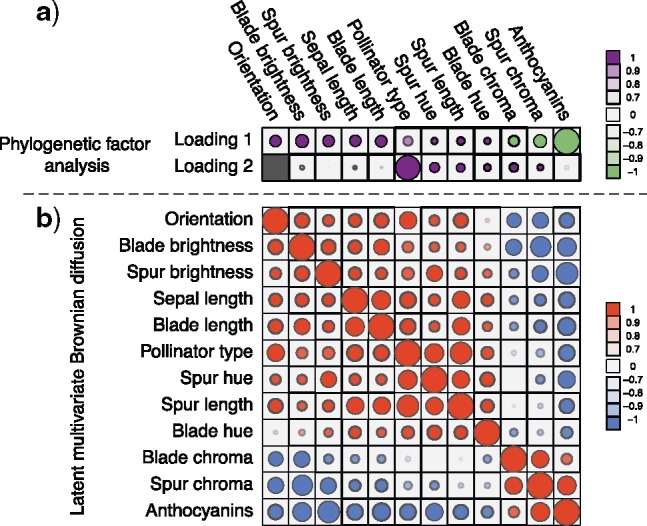
Processes driving columbine flower evolution inferred through PFA or LMBD. a) Loadings estimates from a factor PFA model. Purple circles represent traits positively associated with traits represented by other purple circles within a loading, and negatively associated with traits represented by green circles within a loading. Similarly, traits represented by green circles are positively associated with traits represented by green circles within a loading. Size represents the magnitude of the value of the loadings. Opacity represents the posterior probability that the sign of the given element is equal to the sign of the posterior mean. The greyed out cell represents a structural 0 introduced for identifiability reasons. The magnitude for anthocyanins and pollinator type is less relevant since those measurements are discrete. b) Correlation matrix estimate from a LMBD model. Red represents positive correlation, blue represents anticorrelation, and opacity represents the absolute difference in posterior probability of being greater than 0 and less than 0. Size of the circle represents the magnitude of the correlation. The PFA captures well two independent processes, while the LMBD groups these processes together.

Ignoring the uncertainty in pollinator trait inclusion for the moment, this partitioning recapitulates the block structure that Cybis et al. (2015) report using an LMBD model and an arbitrary thresholding on the posterior mean estimates of the individual pairwise correlation entries in . However, in Figure 1 we quantify the LMBD uncertainty by shading our inference using the same probability measure as we do for our PFA model. Taking correlation uncertainty into consideration we see that, for example the LMBD model would assert that there is no correlation between blade chroma and spur hue. The PFA model by contrast offers the more nuanced assessment that these traits are related through two independent underlying processes, one process of which has a positive association between these traits, the other of which has a negative association.

In addition to improved uncertainty quantification in the block structure of traits, our PFA returns a second independent evolutionary process that relates pollinator with spur length and, in addition, spur and blade chroma and hue, with posterior probability approaching . The existence of two distinct processes, one of which directly connects pollinator and spur length, sheds additional insight into the original hypothesis that Whittall and Hodges (2007) pose. The LMBD model fails to pick up on this, in addition to returning a worse fit to the data.

Transitions to Placental Reproduction

The freshwater fish Poeciliidae represent a family of model organisms in which one can study the transition from nonplacental to placental reproduction and the evolutionary pressures associated with placental introduction. Pollux et al. (2014) define a matrotrophy index to be the log-ratio of the dry weight of newborn fish to the dry weight of eggs at fertilization as a proxy measure of how reliant a fish species is on its placenta for reproduction. Using phylogenetic generalized least squares (PGLS) (Ives and Garland 2010), Pollux et al. (2014) find that Poeciliidae dichromatism, courtship behavior, superfetation, and a sexual selection index are all correlated over evolutionary history with the matrotrophy index. Unlike PFA, PGLS as used by Pollux et al. (2014) does not adjust for potential evolutionary relationships between the traits. Failure to do so can lead to false positive measures of association between individual traits and the matrotrophy index.

Pollux et al. (2014) collect from the literature or measure 14 life-history traits and compile from GenBank or sequence 28 different genes across Poeciliidae species. In our analysis, we only use traits since three of the original traits are functions of the included ones. Of these traits, five are discrete-valued: dimorphic coloration (dichromatism), courtship behavior, superfetation, the presence or absence of ornamental display traits and a count composite of the presence or absence of three other male behaviors (sexual selection index). Six are continuous-valued: log weight and log length for males and females, gonopodium length, and matrotrophy index. Considering species with at least one trait measurement, there are taxa, for which we assume the same fixed phylogenetic tree that Pollux et al. (2014) estimate and similarly condition on in their PGLS analysis. Importantly, 182 trait measurements remain missing. We treat these measurements as missing-at-random in our PFA and do not need to further prune the tree or impute values that may further introduce bias.

Pollux et al. (2014) find that dichromatism, courtship behavior, superfetation, and sexual selection index are all correlated with the matrotrophy index. Figure 2 shows that this concurs with the results of a factor PFA. This small model fit also highlights a weakness of traditional factor analysis assumptions that fix the diagonal elements of the loadings matrix to be positive. In particular, dichromatism is unrelated to the other traits in the second factor, while the positivity constraint would have forced its inclusion. However, the most probable number of independent evolutionary processes is or , with a log Bayes factor in favor over of and a log Bayes factor in favor of over of (Table 1). Since a log Bayes factor of only separates the and models, we include both models in our results, and the data strongly support these PFA models over the LMBD model (log Bayes factor 92).

Figure 2.

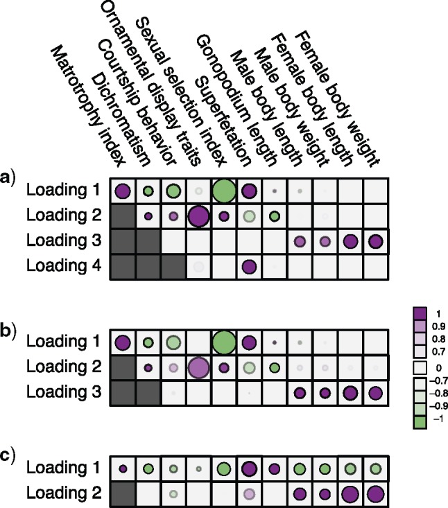
Processes driving transitions to placental reproduction inferred through PFAs. Loading estimates from the a) , b) and c) factor models. Loadings size, coloring and density follow those of Figure 1. Note that the magnitude for dichromatism, courtship behavior, ornamental display traits, sexual selection index, and superfetation is less relevant since those data are discrete. We include the two factor model for direct comparison to the results of Pollux et al. (2014). Loadings in the more probable and factor models do not support an association between matrotrophy index and gonopodium length nor body weights and lengths.

Loadings for the independent evolutionary process factors and under the and PFA models, respectively, recapitulate a negative association between the matrotrophy index and dichromatism, courtship behavior, and sexual selection index, and a positive association with superfetation (Fig. 2, first loading). Uncertainty measures are for all of these trait-factor relationships. However, unlike in Pollux et al. (2014), the PFA does not recover with high posterior probability a relationship between matrotrophy index and gonopodium length nor with body weights and lengths, suggesting that these were false positive findings. For both PFA models, second independent processes and drive dichromatism, courtship behavior, ornamental display traits and sexual selection index positively and superfetation and gonopodium length negatively, where for each of these relationships except involving superfetation () and for courtship behavior in (). Both models also identify similar third independent processes and relating body lengths and weights. We do however find more posterior certainty in the relationships (all ) than in the relationships (all ). It is perhaps surprising that these size measurements are unrelated to any of the other reproductive characteristics. The only marked difference between the and factor models exists in the presence of a fourth evolutionary process in the factor model that controls the presence or absence of superfetation independently of all other traits.

The precision elements for both the and factor models are all significantly greater than 1 and therefore indicate that, for both models, our PFA provides good insight into the relationship of the continuous traits (Table 2). Further, the precision elements are in broad agreement between the and factor models, as we expect due to the negligible difference in marginal likelihoods.

Frequentist-based factor analysis is only identifiable if the number of parameters inferred for a variance/covariance matrix is greater than the number of parameters that need to be inferred for the factor analysis. Interestingly, our PFA model produces interpretable results in spite of the fact that the correlation model has 66 free parameters as opposed to 333 free parameters for the factor model, and 436 free parameters for the factor model.

Triggerfish Fin Shape

The fish family Ballistidae, commonly know as triggerfish, live mostly in reefs; however, the particular part of the reef in which they live can vary. This variability affects not only their diet, but also their mobility needs that fin shapes well reflect (Dornburg et al. 2011). To model shape changes through evolution, phylogenetic morphometrics often relies heavily on PCA (Revell 2009; Polly et al. 2013). However, deterministic data reduction via PCA can introduce bias (Uyeda et al. 2015) and, more importantly, inference of principal components while simultaneously adjusting for an uncertain evolutionary history remains a continuing challenge. PFA offers an alternative approach.

For triggerfish species, Dornburg et al. (2011) sequence and align 12S (833 nucleotides, nt) and 16S (563 nt) mitochondrial genes and RAG1 (1471 nt), rhodopsin (564 nt) and Tmo4C4 (575 nt) nuclear genes, and Dornburg et al. (2008) digitally photograph and mark 13 semilandmark Cartesian coordinates for pectoral, dorsal, and anal fins, generating measurements per species. Among these morphometric measurements, the species Balistapus undulatus is missing dorsal and anal fins landmarks, and the species Rhinecanthus assasi lacks pectoral fin landmarks. For these, we assume the missing data are missing at random.

To accommodate phylogenetic uncertainty within , we concatenate gene alignments into and model nucleotide sequence substitution along the unknown evolutionary history through the Hasegawa et al. (1985) continuous-time Markov chain with unknown transition:transversion rate ratio and stationary distribution . We incorporate across-site rate variation using a discretized, one-parameter Gamma distribution (Yang 1994) with unknown shape and proportion of invariant sites. To specify prior , we make relatively uninformative choices, documented in the BEAST extensible markup language (XML) file in the Supplementary material available on Dryad at http://dx.doi.org/10.5061/dryad.6320t.

These triggerfish sequences and traits favor the factor model with a log Bayes factor of over the factor model and over the factor model (Table 1). Further, these data favor the factor model over the multivariate Brownian diffusion (MBD) model with a log Bayes factor of . Even if this support were equivocal, we caution against using a MBD to model these traits. The unknown variance matrix carries degrees-of-freedom that dwarfs the possible measurements.

For two of the five factors in the model, Figure 3 demonstrates how fin shape changes as a function of latent factor values. We vary and between and that approximates their highest posterior density range over their reconstructed evolutionary history. For , increasing values lead to dorsal and anal fins that become less pointed and more rounded. For , increasing values lead to a counterclockwise rotation of the dorsal fin. Our credible band decreases in size as the factor value gets closer to 0 since the standard deviation of the posterior inference on our loadings is multiplied by these factor values as well.

Figure 3.

Expected triggerfish fin shape given a range of a) first factor values and b) third factor values , holding all others constant. Purple dots estimate semilandmark locations. Green lines are interpolated to present a clearer outline of the fin shape. For the relation represented by the dorsal and anal fins go from more pointed to less pointed. For the relation represented by we see a rotation in the pectoral fin.

We also include the corresponding maximum clade credibility (MCC) tree, colored by factor value, with purple representing positive values and green representing negative values for the first factor and the blue representing positive factor values and orange representing negative factor values for in Figure 4. This tree shows us that the species Balistes polylepsis and B. vetula, have negative factor values for , but those species as well as the rest of the clade with the genus Balistes and species Pseudobalistes fuscus have positive factor values for whereas the clade containing the genus Rhinecanthus has negative factor values for but a close to 0 factor value for . Conversely, the genus Xanthichthys has a negative factor value for and a closer to 0 factor value for We also display posterior clade probabilities for those clades with probability 99%.

Figure 4.

Evolution of independent factors driving triggerfish fin morphology along inferred phylogeny. The colorings display contemporary and ancestral first and third factor values under a factor PFA model. For , green represents positive values and purple represents negative values. For , the scale is orange to blue. The Supplementary material available on Dryad contains plots for , and . Balistes polylepis and Balistes vetula have negative factor values for the first factor whereas the clade containing genus Rhinecanthus has positive factor values. In the third factor , the Balistes genus and the species Pseudobalistes fuscus have positive factor values whereas the genus Rhinecanthus has near 0 factor values. Conversely, the genus Xanthichthys has a negative factor value for , and has a near 0 value for . We display the posterior clade probabilities for probabilities 99%.

For brevity, we have only considered two factors in this section. We selected and since these factors relate distinctive information, however we include the results for the remaining factors in the Supplementary material available on Dryad. We additionally include our inference on the precision elements as well as our results on the inference on the other aspects of our tree model in the Supplementary material available on Dryad.

Lastly, PFA facilitates ancestral shape reconstruction. Figure 5 depicts inferred pectoral, dorsal and anal fin shapes for ancestors of Xanthichthys mento and Balistes capriscus at arbitrary points into their evolutionary past. We choose reconstructions at the MRCA of all 24 species in our study and , and of the expected sequence substitution distance between the MRCA and both contemporaneous species. Typically, high aspect ratio fins, or long fins with a small area, are associated with swimming quickly over large distances. The diet of Xanthichthys mento consists mostly of plankton and swims above reefs and has a high aspect ratio, perhaps reflecting a need to hunt down more evasive prey. We see that these low aspect ratio dorsal and anal fins arose from a moderate MRCA which flatten as the species evolved. The pectoral fin rotated clockwise as this species evolved. In contrast, Balistes capriscus has low aspect ratio dorsal and anal fins, reflecting the fact that it swims more towards the reef floors which may be more useful in navigating the complex habitat. This species evolved from a species with a moderate aspect ratio in its dorsal and anal fins which became broader and more pointed as it evolved. However, the aspect ratio increases again about of the way through its evolution. The pectoral fin rotated counterclockwise as it evolved.

Figure 5.

Inferred ancestral fin shapes at the MRCA and , and of the expected substitution distance between the MRCA and two contemporaneous triggerfish species. In a), Xanthichthys mento has a flat dorsal and anal fin with a point, and a clockwise rotated pectoral fin relative to its ancestors. The dorsal and anal fins become rounder and the pectoral fin rotates counterclockwise moving backwards in time. In contrast, in b), Balistes capriscus has a broad pointed dorsal and anal fin, and a counterclockwise anal fin. The dorsal and anal fins become more pointed and then round out, while the pectoral fin rotates clockwise.

This ancestral reconstruction can provide new insights into the trajectories of shape change that could be further investigated with biomechanical and fluid dynamic models.

Simulation

We briefly evaluate the performance of PFA in estimating the number of factors and loadings matrix under conditions similar to the Aquilegia example. Assuming and fixing and to their posterior mean estimates for the traits and using the fixed tree from this example, we simulate 100 dataset replicates under the PFA model. For each replicate, we then perform posterior inference and, collectively, examine our ability to recover the true generative values.

Under these simulation conditions, we recover the true number of factors with relatively high probability (0.89). With the remaining probability, we recover the more parsimonious model. Averaged across all entries in , we achieve 79.1% coverage using the 95% highest probability density (HPD) interval estimates; while slightly below nominal, this coverage stands as reasonable in practice, especially since HPD intervals incorporate prior information and, in general, return no frequentist guarantees. We also consider the power to detect an uncertainty measure and find that we deem an arbitrary loading entry significant only with probability . However, the magnitude of the entries in vary widely in our examples. Supplementary Figure S5 available on Dryad describes how the true value of influences coverage, power and mean-squared bias. As expected given a prior centered around , coverage is lowest for the largest values of (e.g., 1.5) and power increases with increasing . Importantly for the interpretation of our results, many loadings entries had , suggesting that their true values were likely larger in magnitude than our posterior estimates under the PFA model.

Computational Aspects

To draw posterior inference, we simulate MCMC chains of between 200M and 1B steps, subsampling every 10K steps to eliminate unnecessary overhead and ensure the rate-limiting computation remains the PFA and L/MBD transition kernels. For path sampling, we employ 100 path points based on the quantiles of a beta random variable (Xie et al. 2011), with warm-started chains of 10M steps at each point. In our examples, the PFA chains generate draws 3- to 5-fold faster than the L/MBD chains. Further, with the relatively large ratio of latent to nonlatent traits in the Aquilegia example, we find an approximately 27-fold larger median effective sample size (ESS) across , and than in the latent components of , demonstrating both faster and more efficient sampling.

Discussion

This article merges traditional factor analysis with phylogenetics to provide a new inference tool for comparative studies. The key connection rests on modeling each factor independently as a Brownian diffusion along a phylogeny. The tool we provide not only serves as a dimension reduction technique in the face of high-dimensional traits, but directly addresses the principal scientific questions that many comparative studies raise—specifically, how many independent evolutionary processes are driving these traits? Set in a Bayesian framework, we succeed in inferring these processes for combinations of discrete and continuous traits through model selection, while simultaneously accounting for missing measurements and possible phylogenetic uncertainty.

To make inference under PFA practical, we develop two new MCMC integration techniques. While we rely on previously proposed Gibbs samplers for integrating the loading matrix and residual trait precisions , we require an original algorithm based on dynamic programming to integrate the factors along the phylogeny efficiently. Second, we extend path sampling through a softening threshold to handle discrete traits, in which their latent support depends on the path location . Such changing support previously has limited marginal likelihood estimation across many Bayesian models with latent random variables to combine discrete and continuous observations.

In examples involving columbine flower and fish families Poeciliidae and Balistidae evolution, inference under the PFA is notably quicker under the presence of latent traits, more interpretable and consistently favored via model selection over competing LMBD/MBD models. Interestingly, this success even holds in the Poeciliidae example, where one might expect an LMBD model to outperform. Here, the number of parameters inferred in the variance matrix is small relative to the number of parameters that form a PFA. The Poeciliidae and Balistidae examples also demonstrate our Bayesian approach’s ability to integrate missing data if we make a simple missing-at-random assumption.

Unlike many univariate comparative methods, the PFA simultaneously adjusts for correlation between all traits. This advantage reveals that some previously identified trait relationships in Poeciliidae evolution may be spurious. Further, as demonstrated in the columbine flower example, the inferred factors and their associated loadings probabilistically cluster traits into independent processes that provide additional scientific insight, often hard to discern from the correlation matrix that a LMBD model provides.

An important computational limitation of PFA arises when the number of taxa is much greater than the number of traits . For the PFA, computational cost of our current MCMC integration scales as , while the cost is for the LMBD / MBD models. Nonetheless, the Poeciliidae example carries and, still, the PFA model integrates about more efficiently due to the example’s large ratio of latent traits. For larger ratios, we are currently devising algorithms that remain linear in as future work.

Arguably, PFA reaches its greatest computational potential when the number of traits stands large relative to the number of taxa—the reputed “large , small ” setting. This setting arises commonly in the field of geometric morphometrics where very long series of Cartesian, (semi) landmark coordinate measurements define the shape of the organism. In our Balistidae example, the PFA identifies a number of independent evolutionary processes driving pectoral, dorsal, and anal fin shapes. With the help of sequence data, the PFA also simultaneously infers the phylogeny and reconstructs ancestral shapes. We believe that morphometrics stands poised as a prime beneficiary of PFA.

One potential extension of this method comes from Lemey et al. (2010), where they place different diffusion rates on different branches. Additionally we can adapt the methods in Gill et al. (2017) that allow us to incorporate inference on drift in our factors whose direction changes at different points in the evolutionary process. Ornstein–Uhlenbeck processes are nested within the union of both methods that are implemented in BEAST and are therefore easily adapted for use in PFA.

Supplementary Material

Data available from the Dryad Digital Repository: http://dx.doi.org/10.5061/dryad.6320t.

Funding

The research leading to these results has received funding from the European Research Council under the European Community’s Seventh Framework Programme (FP7/2007-2013) under Grant Agreement No. 278433-PREDEMICS and ERC Grant Agreement No. 260864 and the National Institutes of Health (R01 AI107034, R01 AI117011, and R01 HG006139) and the National Science Foundation (DMS 1264153).

APPENDIX

PFA Gibbs Sampling

While the Gibbs samplers for a standard factor analysis are known and well documented (Lopes and West 2004), there are two aspects of our phylogenetic model that differ sufficiently to require a fresh look at how to draw posterior inference. First, our prior on is based on a phylogenetic tree and therefore requires particular consideration in order to produce an efficient Gibbs sampler. Second, our inference on uses a path sampling approach where we need to infer and at each point along the path and deriving a Gibbs sampler that works for any point in the path will aid this process.

Sampling factors.—

In a standard Bayesian factor analysis, the prior on each element is and so the entire matrix can be Gibbs sampled efficiently in a single step (Lopes and West 2004). For the PFA model, the prior on the factors is defined by Brownian motion on a phylogenetic tree as defined in (6). Thus the conditional density of in our model is proportional to

(A.1)

This expression does not appear to represent a distribution from which we can easily sample, principally stemming from the fact that is a between-column precision and is a between-row precision.

Fortunately, Cybis et al. (2015) devise a pre-order tree-traversal algorithm to determine the conditional distribution of the factors at a single tip given all other tip values. This distribution is multivariate normal with conditional mean and conditional precision . Further, in order to numerically estimate at any point along the path we define

(A.2)

Substituting in the appropriate densities and completing the square, we find that this path is proportional to

(A.3)

where

(A.4)

and

(A.5)

Equation (A.3) is proportional to the density of a ; therefore, in order to sample at a particular point in the path we can draw a row from the distribution .

Sampling loadings.—

The loadings matrix can be Gibbs sampled using the same method described by Lopes and West (2004) with an additional adaptation for use in path sampling. For the examples provided in this paper, we place a prior on each cell in the loadings matrix; however, in this section we prove the Gibbs Sampler for a generic prior. To begin, we again define for a point on the path

(A.6)

Plugging in the proper values for the sampling density and priors, rearranging and completing the square, we find that

(A.7)

where , is a matrix of 1’s with the same dimensions as ,

(A.8)

and

(A.9)

Hence we find the expression in (A.7) is proportional to a product of independent densities. Therefore, if we wish to numerically sample a loadings column at a point on the path then we can sample from the distribution . Since the densities across columns are independent, we may sample from them in parallel.

Sampling residual precision.—

We wish to sample at any point in our path . Let be a matrix equivalent to with rows and columns corresponding to discrete traits removed. We then say that where models continuous trait and is the number of continuous traits in our model. If we define and as the matrices and with the columns corresponding to discrete traits removed, then we can say Our prior on is i.i.d. for different values of and has distribution For an arbitrary point in our path we then define

(A.10)

with density

(A.11)

The expression in (A.11) is proportional to the density of a gamma random variable, and therefore we can sample from this gamma distribution in order to sample at a given point in the path.

References

- Adams D. 2014. A method for assessing phylogenetic least squares models for shape and other high-dimensional multivariate data. Evolution 68(9): 2675–2688. [DOI] [PubMed] [Google Scholar]
- Aguilar O.,, West M. 2000. Bayesian dynamic factor models and portfolio allocation. J. Bus. Econ. Stat. 18:338–357. [Google Scholar]
- Baele G.,, Lemey P.,, Bedford T.,, Rambaut A.,, Suchard M.A.,, Alekseyenko A.V. 2012. Improving the accuracy of demographic and molecular clock model comparison while accommodating phylogenetic uncertainty. Mol. Biol. Evol. 29:2157–2167. [DOI] [PMC free article] [PubMed] [Google Scholar]
- Baele G.,, Lemey P.,, Suchard, M.A. 2016. Genealogical working distributions for Bayesian model testing with phylogenetic uncertainty. Syst. Biol. 65:250–264. [DOI] [PMC free article] [PubMed] [Google Scholar]
- Beguin A.,, Glas C. 2001. MCMC estimation and some model-fit analysis of multidimensional IRT models. Psychometrika 66:541–562. [Google Scholar]
- Clavel J.,, Escarguel G.,, Merceron G. 2015. mvMORPH: an r package for fitting multivariate evolutionary models to morphometric data. Methods Ecol. Evol. 6:1311–1319. [Google Scholar]
- Cybis G.,, Sinsheimer J.,, Bedford T.,, Mather A.,, Lemey P.,, Suchard, M. 2015. Assessing phenotypic correlation through the multivariate phylogenetic latent liability model. Ann. Appl. Stat. 9:969–991. [DOI] [PMC free article] [PubMed] [Google Scholar]
- Dornburg A.,, Santini F.,, Alfaro, M. E. 2008. The influence of model averaging on clade posteriors: an example using the triggerfishes (family Balistidae). Syst. Biol. 57:905–919. [DOI] [PubMed] [Google Scholar]
- Dornburg A.,, Sidlauskas B.,, Santini F.,, Sorenson L.,, Near T.J.,, Alfaro M.E. 2011. The influence of an innovative locomotor strategy on the phenotypic diversification of triggerfish (family: Balistidae). Evolution 65:1912–1926. [DOI] [PubMed] [Google Scholar]
- Drummond A.J.,, Suchard M.A.,, Rambaut A. 2012. Bayesian phylogenetics with BEAUti and the BEAST 1.7. Mol. Biol. Evol. 29:1969–1973. [DOI] [PMC free article] [PubMed] [Google Scholar]
- Felsenstein J. 1973. Maximum likelihood and minimum-steps methods for estimating evolutionary trees from data on discrete characters. Syst. Zool. 22:240–249. [Google Scholar]
- Felsenstein, J. 1985. Phylogenies and the comparative method. Am. Nat. 125:1–15. [Google Scholar]
- Freckleton R.P. 2012. Fast likelihood calculations for comparative analyses. Methods Ecol. Evol. 3:940–947. [Google Scholar]
- Friel N.,, Pettitt, A.N. 2008. Marginal likelihood estimation via power posteriors. J. R. Stat. Soc. Series B Stat. Methodol. 70:589–607. [Google Scholar]
- Gelman A.,, Meng, X.-L. 1998. Simulating normalizing constants: from importance sampling to bridge sampling to path sampling. Stat. Sci. 13:163–185. [Google Scholar]
- Geweke J.,, Zhou, G. 1996. Measuring the pricing error of the arbitrage pricing theory. Rev. Financ. Stud. 9:557–587. [Google Scholar]
- Ghosh J., Dunson, D.B. 2009. Default prior distributions and efficient posterior computation in Bayesian factor analysis. J. Comput. Graph. Stat. 18(2): 306–320. [DOI] [PMC free article] [PubMed] [Google Scholar]
- Gill M.S.,, Ho L.S.T.,, Baele G.,, Lemey P.,, Suchard M.A. 2017. A relaxed directional random walk model for phylogenetic trait evolution. Syst. Biol. 66:299–319. [DOI] [PMC free article] [PubMed] [Google Scholar]
- Hasegawa M.,, Kishino H.,, Yano, T. 1985. Dating of human-ape splitting by a molecular clock of mitochondrial DNA. J. Mol. Evol. 22:160–174. [DOI] [PubMed] [Google Scholar]
- Heaps S.E.,, Boys R.J.,, Farrow M. 2014. Computation of marginal likelihoods with data-dependent support for latent variables. Comput. Stat. Data Anal. 71:392–401. [Google Scholar]
- Huelsenbeck J.P.,, Rannala B. 2003. Detecting correlation between characters in a comparative analysis with uncertain phylogeny. Evolution 57:1237–1247. [DOI] [PubMed] [Google Scholar]
- Ives A.R.,, Garland T., Jr 2010. Phylogenetic logistic regression for binary dependent variables. Syst. Biol. 59:9–26. [DOI] [PubMed] [Google Scholar]
- Jeffreys H. 1935. Some tests of signficance, treated by the theory of probability. Proc. Cambridge Philos. Soc. 29:83–87. [Google Scholar]
- Lemey P.,, Rambaut A.,, Welch J.J.,, Suchard, M.A. 2010. Phylogeography takes a relaxed random walk in continuous space and time. Mol. Biol. Evol. 27:1877–1885. [DOI] [PMC free article] [PubMed] [Google Scholar]
- Liu J.S.,, Wong W.H.,, Kong A. 1995. Covariance structure and convergence rate of the Gibbs sampler with various scans. J. R. Stat. Soc. Series B Stat. Methodol. 57(1): 157–169. [Google Scholar]
- Lopes H.F.,, West M. 2004. Bayesian model assessment in factor analysis. Stat. Sin. 14:41–67. [Google Scholar]
- Newton M.A.,, Raftery A.E. 1994. Approximate Bayesian inference with the weighted likelihood bootstrap. J. R. Stat. Soc. Series B Stat. Methodol. 56:3–48. [Google Scholar]
- Pollux B.J.A.,, Meredith R.W.,, Springer M. S., N R.D. 2014. The evolution of the placenta drives a shift in sexual selection in livebearing fish. Nature 513:233–236. [DOI] [PubMed] [Google Scholar]
- Polly P.D.,, Lawing A.M.,, Fabre A.-C.,, Goswami A. 2013. Phylogenetic principal components analysis and geometric morphometrics. Hystrix, Ital. J. Mammal. 24:33–41. [Google Scholar]
- Pybus, O. G., Suchard, M. A. Lemey, P. Bernardin, F. J. Rambaut, A. Crawford, F. W. Gray, R. R. Arinaminpathy, N. Stramer, S. L. Busch, M. P. and Delwart. E. L.. 2012. Unifying the spatial epidemiology and molecular evolution of emerging epidemics. Proc. Natl. Acad. Sci. 109:15066–15071. [DOI] [PMC free article] [PubMed] [Google Scholar]
- Quinn K.M. 2004. Bayesian factor analysis for mixed ordinal and continuous responses. Polit. Anal. 12:338–353. [Google Scholar]
- Rai P.,, Daume H. 2008. The infinite hierarchical factor regression model. Adv. Neural Inf. Process. Syst. 21:1321–1328. [Google Scholar]
- Revell L.J. 2009. Size-correction and principal components for interspecific comparative studies. Evolution 63:3258–3268. [DOI] [PubMed] [Google Scholar]
- Santos J.C. 2009. The implementation of phylogenetic structural equation modeling for biological data from variance-covariance matrices, phylogenies, and comparative analyses [Master’s thesis]. University of Texas at Austin. [Google Scholar]
- Stephens M. 2000. Dealing with label switching in mixture models. J. R. Stat. Soc. Series B Stat. 62:795–809. [Google Scholar]
- Suchard M.A.,, Weiss R.E.,, Sinsheimer J. S. 2001. Bayesian selection of continuos-time Markov chain evolutionary models. Mol. Biol. Evol. 18:1001–13. [DOI] [PubMed] [Google Scholar]
- Uyeda J.C.,, Caetano D.S.,, Pennell M.W. 2015. Comparative analysis of principal components can be misleading. Syst. Biol. 64:677–689. [DOI] [PubMed] [Google Scholar]
- Vrancken B.,, Lemey P.,, Rambaut A.,, Bedford T.,, Longdon B.,, Günthard H.F.,, Suchard, M.A. 2015. Simultaneously estimating evolutionary history and repeated traits phylogenetic signal: applications to viral and host phenotypic evolution. Methods Ecol. Evol. 6:67–82. [DOI] [PMC free article] [PubMed] [Google Scholar]
- Whittall J.B.,, Hodges, S.A. 2007. Pollinator shifts drive increasingly long nectar spurs in columbine flowers. Nature 447:706–709. [DOI] [PubMed] [Google Scholar]
- Xie W.,, Lewis P.O.,, Chen M.-H. 2011. Improving marginal likelihood estimation for Bayesian phylogenetic model selection. Syst. Biol. 60:150–160. [DOI] [PMC free article] [PubMed] [Google Scholar]
- Yang Z. 1994. Maximum likelihood phylogenetic estimation from DNA sequences with variable rates over sites: approximate methods. J. Mol. Evol. 39:306–314. [DOI] [PubMed] [Google Scholar]