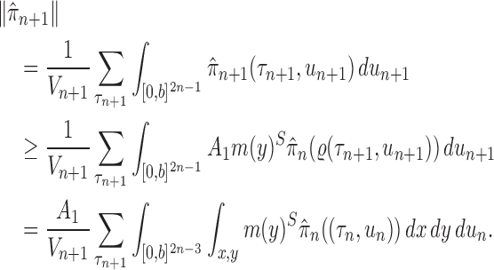
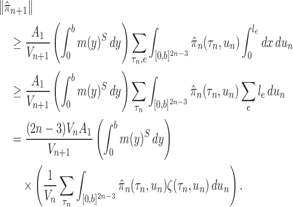
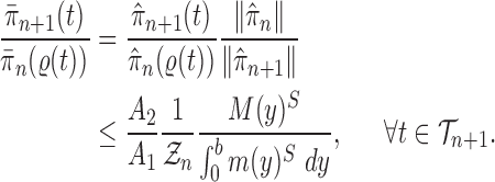
Abstract
Phylogenetics, the inference of evolutionary trees from molecular sequence data such as DNA, is an enterprise that yields valuable evolutionary understanding of many biological systems. Bayesian phylogenetic algorithms, which approximate a posterior distribution on trees, have become a popular if computationally expensive means of doing phylogenetics. Modern data collection technologies are quickly adding new sequences to already substantial databases. With all current techniques for Bayesian phylogenetics, computation must start anew each time a sequence becomes available, making it costly to maintain an up-to-date estimate of a phylogenetic posterior. These considerations highlight the need for an online Bayesian phylogenetic method which can update an existing posterior with new sequences. Here, we provide theoretical results on the consistency and stability of methods for online Bayesian phylogenetic inference based on Sequential Monte Carlo (SMC) and Markov chain Monte Carlo. We first show a consistency result, demonstrating that the method samples from the correct distribution in the limit of a large number of particles. Next, we derive the first reported set of bounds on how phylogenetic likelihood surfaces change when new sequences are added. These bounds enable us to characterize the theoretical performance of sampling algorithms by bounding the effective sample size (ESS) with a given number of particles from below. We show that the ESS is guaranteed to grow linearly as the number of particles in an SMC sampler grows. Surprisingly, this result holds even though the dimensions of the phylogenetic model grow with each new added sequence.
Keywords: Bayesian inference, effective sample size, online inference, phylogenetics, sequential Monte Carlo, subtree optimality
Maximum likelihood and Bayesian methods currently form the most popular means of phylogenetic inference. The Bayesian methods in particular enjoy the flexibility to incorporate a wide range of ancillary model features such as geographical information or trait data which are essential for some applications (Lemey et al., 2009; Ronquist et al., 2012). However, Bayesian tree inference with current implementations is a computationally intensive task, often requiring days or weeks of CPU time to analyze modest data sets with 100 or so sequences.
New developments in DNA and RNA sequencing technology have led to sustained growth in sequence data sets. This advanced technology has enabled real time outbreak surveillance efforts, such as ongoing Zika, Ebola, and foodborne disease sequencing projects, which make pathogen sequence data available as an epidemic unfolds (Gardy et al., 2015; Quick et al., 2016). In general, these new pathogen sequences arrive one at a time (or in small batches) into a background of existing sequences. Most phylogenetic inferences, however, are performed “from scratch” even when an inference has already been made on the previously available sequences. Projects such as  (Neher and Bedford, 2015) incorporate new sequences into trees as they become available, but do so by recalculating the phylogeny from scratch at each update using a fast approximation to maximum likelihood inference, rather than a Bayesian method.
Thus, modern researchers using phylogenetics are in the situation of having previous inferences, having new sequences, and yet having no principled method to incorporate those new sequences into existing inferences. Existing methods either treat a previous point estimate as an established fact and directly insert a new sequence into a phylogeny (Matsen et al., 2010; Berger et al., 2011) or use such a tree as a starting point for a new maximum-likelihood search (Izquierdo-Carrasco et al., 2014). There is currently no method to update posterior distributions on phylogenetic trees with additional sequences.
In this article, we develop the theoretical foundations for an online Bayesian method for phylogenetic inference based on Sequential and Markov Chain Monte Carlo (MCMC). Unlike previous applications of Sequential Monte Carlo (SMC) to phylogenetics (Bouchard-Côté et al., 2012; Bouchard-Côté, 2014; Wang et al., 2015), we develop and analyze online algorithms that can update a posterior distribution as new sequence data becomes available. We first show a consistency result, demonstrating that the method samples from the correct distribution in the limit of a large number of particles in the SMC. Next, we derive the first reported set of bounds on how phylogenetic likelihood surfaces change when new sequences are added. These bounds enable us to characterize the theoretical performance of sampling algorithms by developing a lower bound on the effective sample size (ESS) for a given number of particles. Surprisingly, this result holds even though the dimensions of the phylogenetic model grow with each new added sequence.
Mathematical Setting
Background and Notation
Throughout this article, a phylogenetic tree is a tree
  with leaves labeled by a set of taxon names (e.g., species names), such that each edge
  is associated with a non-negative number
  . These trees will be unrooted, although sometimes a root will be designated for notational convenience. For each phylogenetic tree
  , we will refer to
  as its tree topology and to
  as the vector of branch lengths. We denote by
  the set of all edges in trees with topology
  ; any edge adjacent to a leaf is called a pendant edge, and any other edge is called an internal edge.
We will employ the standard likelihood-based framework for statistical phylogenetics on discrete characters under the common assumption that alignment sites are independently and identically distributed (IID) (Felsenstein, 2004), which we now review briefly. Let  denote the set of character states and let
  . For DNA
  and
and  . We assume that the mutation events occur according to a continuous time Markov chain on states
  with instantaneous rate matrix
  and stationary distribution
  . This rate matrix
  and the branch length
  on the edge
  define the transition matrix
  on edge
  , where
  denotes the probability of mutating from state
  to state
  across the edge
  (with length
  ).
).
In an online setting, the taxa  and their corresponding observed sequences
  , each of length
  , arrive in a specific order, where
  is a finite but large number. For all
  , we consider the set of all phylogenetic trees that have
  as their set of taxa and seek to sample from a sequence of probability distributions
  of increasing dimension corresponding to phylogenetic likelihood functions (Felsenstein, 2004).
For a fixed phylogenetic tree  , the phylogenetic likelihood is defined as follows and will be denoted by
  . Given the set of observations
  of length
  up to sequence
  , the likelihood of observing
  given the tree has the form
 |
where  ranges over all extensions of
  to the internal nodes of the tree,
  denotes the assigned state of node
  by
by  , and
, and  denotes the root of the tree. Although we designate a root for notational convenience, the methods and results we discuss apply equally to unrooted trees.
Given a proper prior distribution with density  imposed on branch lengths and tree topologies, the target posterior distributions have densities
  . We will also use
  to denote the unnormalized density
  Throughout the article, we assume that the phylogenetic trees of interest all have non-negative branch lengths bounded from above by
  and use
  to denote the set of all such trees.
An important goal of this article is to show that the collection of particles generated by the online phylogenetic sequential Monte Carlo (OPSMC) algorithm do a good job of approximating a sample from the posterior distribution, in the same way that a sample from a MCMC algorithm approximates a sample from the posterior. We would like to show that this approximation becomes arbitrarily good as the number of particles goes to infinity, that is, that the particle distribution converges to the posterior distribution. The type of convergence we will demonstrate is called weak convergence, which means here that for any integrable real-valued function  defined on the set of trees, the weighted average of the value of the function
  over the trees
  and corresponding weights generated by the algorithm converges (with probability 1) to the to the posterior mean of
  . This convergence result also implies weak convergence of many key quantities of interest in phylogenetics: convergence of posterior probabilities on trees, branch lengths, and splits.
The proofs require a slightly more abstract measure-theoretic perspective. A measure in this context is a function from subsets of some set to the non-negative real numbers with nice properties, such as that the measure of a countable union of disjoint sets is the sum of the measures of the individual sets. A classic example is Lebesgue measure on subsets of real space, which simply gives the volume of each subset. We can extend this to  , the product space of the space of all possible tree topologies and the space of all branch lengths
  , via the corresponding product measure,
  , that is uniform on trees and Euclidean on each branch length space. In our presentation, we will use the notation
  to denote the integration of a test function
  (defined on
  ) with respect to the measure
  . Specifically, this integration can be computed by
 |
for any  and test function
  defined on
  , where
  is the number of different topologies of
  . A posterior distribution on
  can also be considered a measure, such that the value of the posterior measure on a subset of
  is simply the integral of the posterior on that subset.
In this article, we will also be considering measures on collections of discrete particles, which are simply non-negative weights on those particles: the measure applied to a collection of particles is the sum of those particle weights. This measure will be called the empirical measure. Thus, said in measure-theoretic terms, we would like to show that the empirical measure on the particles converges weakly to the posterior measure on  .
.
Sequential Monte Carlo
SMC methods are designed to approximate a sequence of probability distributions changing through time. These probability distributions may be of increasing dimension or complexity. They track the sequence of probability distributions of interest by producing a discrete representation of the distribution  at each generation
  through a random collection of weighted particles. In the online phylogenetic context, these particles are trees; after each generation, new sequences arrive, and the collection of particles is updated to represent the next target distribution.
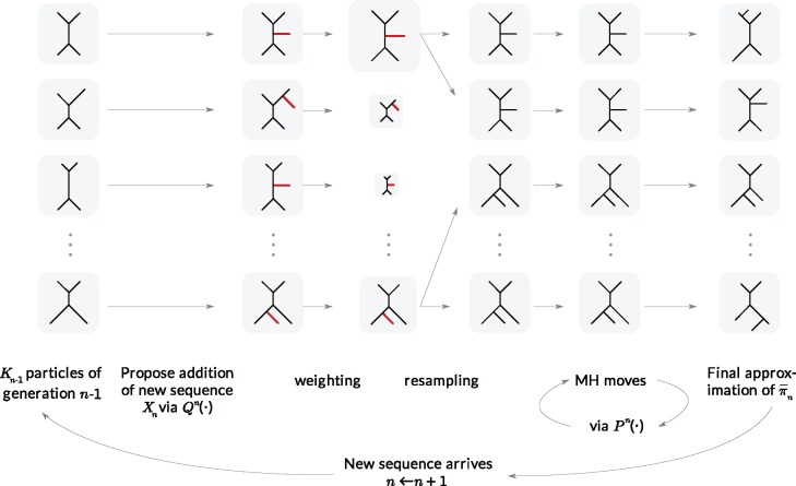
To make it easier to keep track of all variables involved in the description of SMC, we also provide a table of variables in the Appendix. Figure 1 can also be used as a reference to the steps of the algorithm. It is worth noting that the algorithm starts with a set of weighted particles, which are illustrated at the center of Figure 1, right before the “resampling step.” While the details of the algorithms might vary, the main idea of SMC interspersed with MCMC sampling can be described as follows.
Figure 1.
An overview of the OPSMC algorithm.
At the beginning of each generation  , a list of
  particles
  are maintained along with a positive weight
  associated with each particle
  . (In our phylogenetic context, each particle at this point is a phylogenetic tree with
  taxa). Using a valid SMC algorithm, the weights of these particles can be normalized to approximate the integral of any integrable test function
  with respect to the target distribution, which in our case is:
 |
(1) |
This approximation will be formalized into a statement about weak convergence of the empirical particle distribution to the target (in our case the phylogenetic posterior).
A new list of  particles is then created in three steps: resampling, Markov transition, and mutation.
Resampling step
The aim of the resampling step is to obtain an unweighted empirical distribution of the weighted measure  by discarding samples with small weights and allowing samples with large weights to reproduce (Fig. 1, “resampling” step). Particle sampling is done in proportion to particle weight, thus from an evolutionary perspective, this is a Wright–Fisher step using particle weights as fitnesses. After resampling, the weights on the particles have effectively been translated into their frequency, and so each particle is then assigned the same weight. A total of
  particles are sampled from the weights
  , and we denote the particles obtained after this step by
  .
.
Markov transition
The scheme employed in the resampling step introduces some Monte Carlo error. Moreover, when the distribution of the weights from the previous generation is skewed, the particles having high importance weights might be oversampled. This results in a depletion of samples (or path degeneracy): after some generations, numerous particles are in fact sharing the same ancestor as the result of a “selective sweep” in the SMC algorithm.
An optional Markov transition step can be employed to alleviate this sampling bias, during which MCMC steps are run separately on each particle  for a certain amount of time to obtain a new approximately independent sample
  (Fig. 1, “MH moves” step). These transitions are done via the Metropolis–Hastings kernel
  , which we will describe in more detail in the next section. Note that in our phylogenetic setting, the dimension of the state space does not change in the Resampling and Markov transition steps, and all particles have the same number of taxa as ones from the original list (
 taxa).
Mutation step
Finally, in the mutation step, new particles  are created from the previous generation
  using a proposal distribution
  (that may be dependent on data). That is, for each
  , the particle
  is independently generated from the proposal distribution
  . The particles are then weighted by an appropriate weight function
  . If we assume further that for each state
  , there exists a unique state, denoted by
  , such that
  , then
  can be chosen as
 |
(2) |
The new particles  with their corresponding weights
  (where
  for
for  ) now represent the distribution
  and act as the input for the next generation.
In our phylogenetic context, this mutation step adds a new sequence to the tree: the new particle  will be
  -taxon tree obtained from the
  -taxon tree
  (Fig. 1, “propose addition of new sequence”). Then
  is simply
  but with the most recently added pendant edge removed. To add a sequence, the proposal strategy
  will specify: an edge
  to which the new pendant edge is added, the position
  on that edge to attach the new pendant edge, and the length
  of the pendant edge. Different ways of choosing
  lead to different sampling strategies and performances. Note that such an addition changes not only the distribution on the state space, but also the state space itself.
The process is then iterated until  .
.
Online Phylogenetic Inference via Sequential Monte Carlo
Next, we more fully develop OPSMC and isolate technical conditions that will ensure a correct sampler. For these conditions, we make a distinction between Criteria, which are a more general set of conditions that imply consistency of OPSMC, and stronger Assumptions, which guarantee that the Criteria hold and to enable further analyses of the sampler.
In contrast to the traditional setting of SMC, for OPSMC when the number of leaves  of the particles increases, not only does the local dimension of the space
  increase linearly, the number of different topologies in
  also increases superexponentially in
  . Careful constructions of the proposal distribution
  , which will build
  -taxon trees out of
  -taxon trees, and the Markov transition kernel
  are essential to cope with this increasing complexity. This goes beyond simply satisfying the criteria guaranteeing a correct sampler (Fourment et al., 2017).
General Criteria for a Consistent OPSMC Sampler
The proposal distributions  will be designed in such a way that the following criterion holds.
Criterion 1.
At every generation of the OPSMC sampling process, for any two trees
and
in the tree space
, the proposal density
satisfies
if and only if
can be obtained from
by removing the taxon
and its corresponding edge.
This formulation is analogous to the definition of “covering” from (Wang et al., 2015), although is distinct in the setting of online inference. In either case, for every tree  , there exists a unique tree
  in
in  such that
  and thus a weight function of the form (2) can be used.
As we mentioned in the previous section, to obtain an  -taxon tree from an
  -taxon tree, a proposal strategy
  must specify:
an edge
 to which the new pendant edge is added,
the position
 on that edge to attach the new pendant edge, and
the length
 of the pendant edge.
The position  on an edge of a tree will be specified by its distal length, which is the distance from the attachment location to the end of the edge that is farthest away from the root of the tree.
Besides the SMC proposal strategy  , an appropriate Markov transition kernel
  can increase the effectiveness of an OPSMC algorithm. It is worth noting that the problem of sample depletion is even more severe for OPSMC than for typical applications of SMC, since after each generation, the sampling space actually expands in dimensionality and complexity. To alleviate this sampling bias, MCMC steps can be run separately on each particle for a certain amount of time to obtain new independent samples. We require the following criterion, which is as expected for any Markov transition kernel used in standard MCMC.
Criterion 2.
At every generation of the OPSMC sampling process, if a Markov transition kernel is used, the Markov transition kernel
has
as its stationary distribution.
As we will see later in the proof of consistency of OPSMC, Criterion 2 is the only assumption required of the Markov transition kernel if it is applied. This leaves us with a great degree of freedom to improve the efficiency of the sampling algorithm without damaging its theoretical properties. For example, one can use global information provided by the population of particles, such as ESS (Beskos et al., 2014), to guide the proposal, or to define a transition kernel on the whole set (or some subset) of particles (Andrieu et al., 2001). In the context of phylogenetics, we can design a sampler that recognizes subtrees that have been insufficiently sampled, and samples more particles to improve the ESS within such regions. Similarly, one can use samplers that rearrange the tree structure in the neighborhood of newly added pendant edges.
We will prove in Theorem 10 that when Criteria 1 and 2 are satisfied, then the OPSMC sampler is consistent.
Designing an Effective OPSMC Sampler
Although Criteria 1 and 2 guarantee the consistency of OPSMC, they do not lead to any insights about the performance of the OPSMC sampler. From a practical point of view, one is interested in quantifying some measure of efficiency of an MCMC algorithm. This question is even more interesting for SMC (and in particular, for phylogenetic SMC algorithms), since in the general case it is known that SMC-type algorithms may suffer from the curse-of-dimensionality: when the dimension of the problem increases, the number of the particles must increase exponentially to maintain a constant effective sample size (Chopin, 2004; Bengtsson et al., 2008; Bickel et al., 2008; Snyder et al., 2008).
In this article, we are interested how the ESS of the OPSMC sampler behaves in the limit of a large number of particles. This task is challenging because we need to quantify how the target distribution changes with newly added sequences, and how the proposals should be designed to cope with these changes in an efficient way. Throughout this section, we will also derive several assumptions, imposed on both the target distribution and the design of the proposal, to enable such analyses.
First we assume the prior distribution does not change drastically when a new taxon is added:
Assumption 3.
There exists
independent of
, and
such that
and
for all
.
In practice, the most common prior distribution on unrooted trees is the uniform distribution on topologies with an identical prior on each of the branches, which satisfy the Assumption 3 with  .
.
As we will discuss in later sections, to make sure that the proposals can capture the posterior distributions  efficiently, some regularity conditions on
  are also necessary. These conditions are formalized in terms of a lower bound on the posterior expectation of
  , the average branch length of
  for a given tree
  :
:
Assumption 4
(Assumption on the average branch length). There exist positive constants
(independent of
) such that for each
where
is the number of tree topologies with
taxa, and
denotes the average of branch lengths of the tree
.
In other words, we assume that on average (with respect to the posterior distribution), the average branch lengths of the trees are bounded from below by  . While the condition is technical, it can be verified in many realistic cases in phylogenetic inference. For example, in the absence of data, the posterior is just the prior, and Assumption 4 holds for any prior that put equal weights on topologies and selects branch lengths from a distribution with nonzero mean. Similarly, if the target distributions concentrate on a single “correct” tree generated from a Yule process with rate parameter
  , then the average branch length converges to
  .
.
As we discussed above, to quantify the efficiency of OPSMC, we need to provide some estimates on how the target distribution changes with newly added sequences. We will discuss in detail below that the most extreme changes on the target distributions happen when some of the target distribution concentrates on a set of trees with short edges, for which a single new sequence can shake up all previous beliefs about the phylogenies of interest. Assumption 4 rules out such pathological behaviors and provides a foundation for analyzing the ESS, although it does impose some limitations. For instance, if we think of a random process generating  taxon trees in a fixed time (e.g., since the dawn of life on earth) then for most natural models, the average branch length might go to zero as
  goes to infinity. However, we note that both Assumptions 3 and 4 can be further relaxed to address more general cases (details in the section “Effective sample sizes of online phylogenetic SMC”).
Throughout the article, we will investigate two different classes of sampling schemes: length-based proposals and likelihood-based proposals.
Length-based proposals
For length-based proposals:
the edge
 is chosen from a multinomial distribution weighted by length of the edges,
the distal position
 is selected from a distribution
  (with density
  ) across the edge length, and
the pendant length
 is sampled from a distribution
  (with density
  ) with support contained in
  .
.
For example, if these  distributions are uniform, we obtain a uniform prior on attachment locations across the tree.
We assume that
Assumption 5.
The densities
of the distal position on edge
and
of the pendant edge lengths are continuous on
and
, respectively and satisfy
where
denotes the length of edge
and
is independent of
.
One way to look at this assumption is that it is designed to guarantee Criterion 1: given two trees  and
and  such that
  can be obtained from
  by removing the taxon
  and its corresponding edge, we want to guarantee that
  is positive. In the length-based proposal, this corresponds to guaranteeing that the proposal does not “miss” any possible choice of the edge, the distal position, and the pendant edge length, and one way to do so is to assume that the densities
  and
and  are bounded away from zero. The assumption is clearly implied by (and so is weaker than) a uniform positive lower bound on the densities
  and
and  . The constant
  in the assumption quantifies how “spread out” the distribution is on
  and plays an important role in the efficiency of the algorithm.
Example 6.
For any density function
on
such that
is integrable, the family of proposals
satisfies Assumption 5.
Likelihood-based proposals
We denote by  the tree obtained by adding an edge of length
  to edge
  of the tree
  at distal position
  . Any tree
  can be represented by
  , where
  is the edge on which the pendant edge containing the most recent taxon is attached. In the likelihood-based approach, the edge
  (from the tree
  ) is chosen from a multinomial distribution weighted by a user-defined likelihood-based utility function
  . Likelihood-based proposals are informed by data and are capable of capturing the posterior distribution more efficiently, but with an additional cost for computing the likelihoods.
In a Bayesian inference framework, the most natural utility function is the average likelihood utility function
 |
In this setting, for a fixed tree  , the utility function on each edge
  of the tree is computed by
  . The utility quantifies the expected value of the unnormalized posterior if we indeed attach the new pendant edge to edge
  . The sampler then uses these weights to choose the edge to attach the new sequence. By doing so, the proposals obtain a set of “better” trees that are more likely to survive in the subsequent generations.
Many other likelihood-based utility functions (that are quicker to compute) can be defined. We will assume that the likelihood-based utility function  satisfies the following assumption.
Assumption 7.
There exist
independent of
such that
for all
.
This assumption ensures that the sampler is efficient as long as the utility function  is “comparable” to the average likelihood utility function up to some multiplicative constants
  and
and  . By analyzing OPSMC under this assumption rather than average likelihood utility function itself, we have the option to choose other (cheaper) utility functions for the proposal, the most important of which is the maximum a posteriori (MAP) utility function
 |
Here, we approximate an integral by the MAP multiplied by the area of integration (in this case,  ). This utility function can be computed via a simple optimization procedure that can be done quickly and efficiently in computational phylogenetics software and avoids the burden of sampling the posterior distribution required to compute the average likelihood utility function. The following lemma (proven in the Appendix) establishes that the MAP utility function also satisfies Assumption 7.
Lemma 8.
There exists
independent of
such that
for all
.
In a similar manner, the distributions  and
and  might also be guided by information about the likelihood function. As for the length-based proposal, we assume the following conditions on the distal position and pendant edge length proposals for the likelihood-based approach.
Assumption 9.
The densities
and
are absolutely continuous with respect to the Lebesgue measure on
and
, respectively. Moreover, there exists
independent of
such that
This condition plays the same roles as Assumption 5 in the length-based proposal: to guarantee Criterion 1 by ensuring that the densities  and
and  are bounded away from zero. Since the likelihood-based proposals are more difficult to analyze than the length-based one, Assumption 9 is a bit stronger than Assumption 5. However, we note that the density functions from Example 6 satisfy both assumptions.
Consistency of Online Phylogenetic SMC
We recall that the OPSMC sampler maintains a list of  particles
  with a positive weight
  associated with each particle
  . We would like to evaluate whether a sample of particles provides a good approximation to the posterior distribution in the sense of (1), which is made rigorous in measure-theoretic terms as follows. We form the normalized empirical measure
  and define the integral
  of a test function
  with respect to this measure by
 |
We will show that the normalized empirical measure  converges weakly to
  , that is the integral
  of a test function
  with respect to this measure converges to the integral of
  with respect to the posterior distribution with probability 1.
In this section, we will demonstrate this weak convergence by induction on the number of taxa  ; that is, for every
  , assuming that
  , we will prove that
  (where
  means weak convergence). We note that although the measures mentioned above are indexed by
  , they implicitly depend on the number of particles from the previous generations. Thus, the convergence should be interpreted in the sense of when the number of particles of all generations approach infinity.
We note that when  , the set of all rooted trees with no taxa consists of a single tree
  . Thus, if we use this single tree as the ensemble of particles at
  , then
  is precisely
  . Alternatively, we can start with
  and use an MCMC method to create an ensemble of particles with stationary distribution
  . In either case, an induction argument gives the main theorem:
Theorem 10
(Consistency). If Criteria 1 and 2 are satisfied and the sampler starts at
by a list consisting of a single rooted tree with no taxa, or at
with an ensemble of particles created by an ergodic MCMC method with stationary distribution
, then
converges weakly to the posterior
. That is, for every integrable test function
and
as
, where a.s. denotes almost sure convergence (i.e., convergence with probability 1).
Theorem 10 shows that approximation by the OPSMC sampler becomes arbitrarily good as the number of particles goes to infinity.
Remark 11.
Theorem 10 describes the asymptotic behavior of OPSMC in the limit when the number of particles of all generations (up to generation
) approaches infinity, and guarantees that the algorithm is consistent regardless of the relative rates with which the
approach infinity. For example, in the traditional setting when the number of particles are the same in every generation, that is,
, we also have
as
.
However, it is worth pointing out that because the sampler is built sequentially, to make a prediction with a given accuracy at generation  with finite data, we need to control the number of particles from all previous generations. These issues will be further addressed in the latter part of the article, where we uniformly bound the ESS of the sampler as the generations proceed.
Characterizing Changes in the Likelihood Landscapes When New Sequences Arrive
Although the consistency of OPSMC is guaranteed, and informative OPSMC samplers can be developed by changing the Markov transition kernels, its applicability is constrained by an implicit assumption: the distance between target distributions of consecutive generations is not too large. Since SMC methods are built upon the idea of recycling particles from one generation to explore the target distribution of the next generation, it is obvious that one would never be able to design an efficient SMC sampler if  and
and  are very different from one another.
While a condition on minor changes in the target distributions may be easy to verify in some applications, it is not straightforward in the context of phylogenetic inference. A similar question on how the “optimal” trees (under some appropriate measure of optimality) change has been studied extensively in the field, with negative results for almost all regular measures of optimality (Heath et al., 2008; Cueto and Matsen, 2011). However, to the best of our knowledge, no work has been done detailing how phylogenetic likelihood landscapes change when new sequences arrive.
In this section, we will establish that under some minor regularity conditions on the distribution described in the previous sections, the relative changes between target distributions from consecutive generations are uniformly bounded. This result enables us to provide a lower bound on the effective sample size of OPSMC algorithms in the next section.
Lemma 12.
Consider an arbitrary tree
obtained from the parent tree
by choosing edge
, distal position
and pendant length
. Denote
and
Recalling that our sequences are of length
and assuming that
for all
, we have
Sketch of proof.
Using the 1D formulation of the phylogenetic likelihood function derived in Dinh and Matsen (2016), we can prove that
(3) Similarly, we have
for all
.
For any tree
with
taxa, we let
and denote by
and
the chosen edge for attaching the last taxon, the distal length, and the length of the pendant edge, respectively. We deduce that
Recall that
is the average branch length of
. Using the fact that for a fixed tree
,
and
, we have
Recalling that
, we deduce that
This completes the proof. □
The main idea of Lemma 12 is to bound the posterior values of a tree  by that of its parent
  with an explicit constant independent of
  . While the proof of the lemma is technical, its main insights can be explained from the observation that the most extreme changes of the posteriors happen when, either (1) the new pendant edge is small, or (2) the edge lengths of the parent tree
  are small.
Indeed, in the simplest case where both priors on the sets of trees with  and
and  -taxa are uniform, we can choose
  . Equation (3) and the subsequent equation establish that the ratio between the likelihood values of tree
  and its parent
  can be bounded from above as long as the length of the pendant edge is not too small. Similarly, the ratio between the total masses of
  and
and  can also be controlled if the target distribution
  does not concentrate on a set of trees with short edges. This motivates Assumption 4 to provide a lower bound on the total edge lengths and to rule out such pathological behaviors.
ESSs of Online Phylogenetic SMC
In this section, we are interested in the asymptotic behavior of OPSMC in the limit of large  , that is, when the number of particles of the sampler approaches infinity. This asymptotic behavior is illustrated via estimates of the ESS of the sampler with large numbers of particles. We note that although there are several studies on the stability of SMC as the generations proceed, most of them focus on cases where the sequence of target distributions have a common state space of fixed dimension (Del Moral, 1998; Douc and Moulines, 2008; Künsch, 2005; Oudjane and Rubenthaler, 2005; Del Moral et al., 2009; Beskos et al., 2014). In general, establishing stability bounds for SMC requires imposing some conditions on the effect of data at any generation
  to the target distribution at generation
  (Crisan and Doucet, 2002; Chopin, 2004; Doucet and Johansen, 2009). Lemma 12 helps validate a condition of this type.
In this section, we use the ESS (Kong et al., 1994; Liu and Chen, 1995) of the particles at generation  as a measure of the sampler’s efficiency. The ESS is computed as
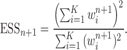 |
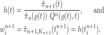
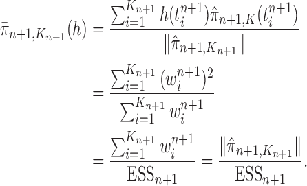
The detailed derivation of the formula is provided in Kong et al. (1994) and Liu and Chen (1995), but a simple intuition is as follows: if the weights of the particles are roughly of the same fitness (weight), then the ESS is equal to the number of particles; on the other hand, if  of the particles share almost all of the weight equally,
  . This formulation of the ESS is usually used to do adaptive resampling, whereas some additional resampling steps are done when the ESS drops below certain threshold. We emphasize that as with other measures of efficiency of MCMC methods, good ESS is necessary but not sufficient to ensure a good quality posterior. From the definition, it is also clear that the ESS could not exceed the number of particles.
The following result, proven in the Appendix, enables us to estimate the asymptotic behavior of the sample’s ESS in various settings.
Theorem 13.
In the limit as the number of particles approaches infinity, we have
with probability 1.
This asymptotic estimate and the results on likelihood landscapes from the previous section allow us to prove the following Theorem (see Appendix for proof).
Theorem 14
(ESS of OPSMC for likelihood-based proposals). If Assumptions 3, 4, 7, and 9 hold, then with probability 1, there exists
independent of
such that
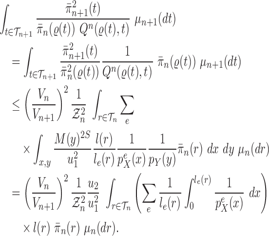
. That is, the effective sample size of an OPSMC sampler with likelihood-based proposals is bounded below by a constant multiple of the number of particles. Moreover, if Assumption 4 does not hold, the ESS of OPSMC algorithms decays at most linearly as the dimension (the number of taxa) increases.
We also have similar estimates for length-based proposals (see Appendix for proof):
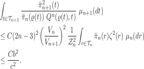
Theorem 15
(ESS of OPSMC for length-based proposals). If Assumptions 3, 5, and 4 hold, then with probability 1, the ESS of OPSMC with length-based proposals are bounded below by a constant multiple of the number of particles. Moreover, if Assumption 4 does not hold, the ESS of OPSMC algorithms decays at most quadratically as the dimension (the number of taxa) increases.
In summary, we are able to prove that in many settings, the ESS of OPSMC is bounded from below. These results are surprising, since in the general case it is known that SMC-type algorithms may suffer from the curse-of-dimensionality: when the dimension of the problem increases, the number of the particles must increase exponentially to maintain a constant ESS (Chopin, 2004; Bengtsson et al., 2008; Bickel et al., 2008; Snyder et al., 2008). We further note that although the Markov transition kernels  after the mutation step are not involved in the theoretical analysis of the ESS in this section, the results hold true for all kernels that satisfy Criterion 2.
Discussion
In this article, we establish foundations for OPSMC, including essential theoretical convergence results. We prove that under some mild regularity conditions and with carefully constructed proposals, the OPSMC sampling algorithm is consistent. This includes relaxing the condition used in (Bouchard-Côté et al., 2012), in which the authors assume that the weight of the particles are bounded from above. We then investigate two different classes of sampling schemes for online phylogenetic inference: length-based proposals and likelihood-based proposals. In both cases, we show the ESS to be bounded below by a multiple of the number of particles.
The consistency and convergence results in this article apply to a variety of sampling strategies. One possibility would be for an algorithm to use a large number of particles, directly using the SMC machinery to approximate the posterior. Alternatively, the SMC part of the sampler could be quite limited, resulting in an algorithm which combines many independent parallel MCMC runs in a principled way. As described above, the SMC portion of the algorithm enables MCMC transition kernels that would normally be disallowed by the requirement of preserving detailed balance. For example, one could use a kernel that focuses effort around the part of the tree which has recently been disturbed by adding a new sequence.
In the future we will develop efficient and practical implementations of these ideas, and a first step in this direction has already been made (Fourment et al., 2017). Many challenges remain. For example, the exclusive focus of this article has been on the tree structure, consisting of topology, and branch lengths. However, Bayesian phylogenetics algorithms typically coestimate mutation model parameters along with the tree structures. Although proposals for other model parameters can be obtained by particle MCMC (Andrieu et al., 2010), we have not attempted to incorporate it into the current SMC framework. In addition, we note that the input for this type of phylogenetics algorithm consists of a multiple sequence alignment (MSA) of many sequences, rather than just individual sequences themselves. This raises the question of how to maintain an up-to-date MSA. Programs exist to add sequences into existing MSAs (Caporaso et al., 2010; Katoh and Standley, 2013), although from a statistical perspective, it could be preferable to jointly estimate a sequence alignment and tree posterior (Suchard and Redelings, 2006). It is an open question how that could be done in an online fashion, although in principle it could be facilitated by some modifications to the sequence addition proposals described here.
Funding
This work was funded by National Science Foundation grants [DMS-1223057, CISE-1564137 to V.D. and F.A.M.]; National Institutes of Health grant [U54-GM111274 to V.D. and F.A.M.]; and Faculty Scholar grant from the Howard Hughes Medical Institute and the Simons Foundation to F.A.M.
Appendix
Notation and variables

|
Particle in generation  , weighted by , weighted by 
|

|
Particle obtained after the “resampling step,” unweighted |

|
Particle obtained after the “Markov transition step,” unweighted |

|
Particle in generation  , obtained after the “mutation step,” weighted by , obtained after the “mutation step,” weighted by 
|

|
Unnormalized measure, induced by the particles 
|

|
Unnormalized measure, induced by the particles 
|

|
Unnormalized measure, induced by the particles 
|

|
Unnormalized measure, induced by the particles 
|

|
The posterior distribution at generation 
|

|
The proposal distribution at generation 
|

|
The Markov transition kernel at generation 
|

|
Proposal distribution of the distal position |

|
Proposal distribution of the pendant edge length |
Integration on 
As described in the introduction, to do integration on  , the product space of the space of all possible tree topologies and the space of all branch lengths
  , we consider the corresponding product measure,
  , that is uniform on trees and Euclidean on each branch length space. Integration using this measure is then just the average of the integrals for each topology:
 |
for any  and test function
  defined on
  , where
  is the number of different topologies of
  .
.
Consistency of Online Phylogenetic SMC
For clarity, we restate below the main steps in the OPSMC and introduce some important notations. We recall that at the beginning of each generation  , a list of
  particles
  are maintained along with a positive weight
  associated with each particle
  . These weighted particles form an unnormalized measure and a corresponding normalized empirical measure
 |
such that  approximates
  . A new list of
  particles is then created in three steps: resampling, Markov transition and mutation.
Resampling step (the “resampling” step illustrated in Fig. 1).
A total of  particles are sampled from the distribution
  , and after resampling we obtain the unweighted measure
 |
where  is the multiplicity of particle
  (i.e., the number of times
  arose in the sample), sampled from a multinomial distribution parameterized by the weights
  . We denote the particles obtained after this step by
  .
.
Markov transition (the “MH moves” step illustrated in Fig. 1). MCMC steps can be run separately on each particle  for a certain amount of time to obtain a new approximately independent sample
  with (unweighted) measure denoted
  .
.
Mutation step (the “propose addition of new sequence” step illustrated in Fig. 1).
In the mutation step, new particles  are created from a proposal distribution
  and are weighted by the weight function
  defined by equation (2). The new particles
  with their corresponding weights now represent the distribution
  and act as the input for the next generation.
The proposal  is assumed to be normalized, and the unnormalized measure over the particles
  can be computed by
 |
for any measurable set  .
.
The process is then iterated until  . For convenience, we will denote the unnormalized empirical measures of the particles right after generation
  by
by  ,
,  and
and  , respectively. Similarly, the corresponding normalized distributions will be denoted by
  ,
,  and
and  .
.
For convenience, let  and
and  be the number of particles at the
  and
and  generations, respectively. Recall that the normalized distributions after the substeps of OPSMC are denoted by
  ,
,  , and
, and  , we have the following lemma.
Lemma 16.
Assume that Criteria 1 and 2 are satisfied. If we define
then the following statements hold, where
means weak convergence
If
, then
.
If
, then
.
If
, then
.
is proportional to
.
If
, then
.
Proof of Lemma 16.
(1). Assume that
converges to
a.s.,
where here
denotes the total mass of the empirical measure
(i.e., the sum of all of all particle weights). Since the particles in generation
are sampled independently from a multinomial distribution with fixed weights, by the strong law of large numbers, we have
This implies
This implies that when
, we have
a.s..
(2). The rationale behind the use of MCMC moves is based on the observation that if the unweighted particles are distributed according to
, then when we apply a Markov transition kernel
of invariant distribution
to any particle, the new particles are still distributed according to the posterior distribution of interest.
Formally, if
a.s. for every integrable test function
, by choosing
for any measurable set
, we deduce that
a.s., since the Markov kernel
is invariant with respect to
. Therefore, for any measurable function
, we have that
converges to
almost surely.
(3). Since
a.s. for every integrable test function
, by choosing
for any measurable set
, we deduce that
Therefore, for any measurable function
, we also have
converges to
almost surely.
(4) We note that
(A.1) (5). Since the proposal
and the Markov kernel
are assumed to be normalized, we have
.
We have,
(A.2) By a similar argument, we have
In other words,
converges to
. □
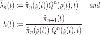
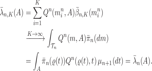
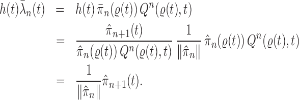
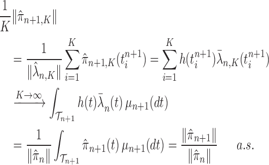
Proof of Theorem 13.
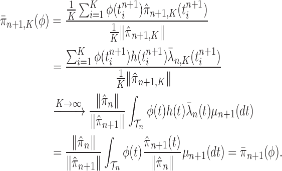
By definition, we have
Thus,
On the other hand, by applying Theorem 10 for
, we have
which completes the proof via the convergence result (A.2). □
An induction argument with Lemma 16 gives the main theorem.
Other Proofs
Proof of Lemma 8.
The lower bound is straightforward. For the upper bound, consider
and fix
; by the same arguments as in the proof of Lemma 12, we have
Thus, if we define
then we have
and
On the other hand, from Lemma 12, we have
.
By choosing
, we obtain
which completes the proof. □
Proof of Lemma 12.
Let
be the length of the edge
and
be the transition matrix across an edge of length
and
the observed value at site
of the newly added taxon. We follow the formulation of 1D phylogenetic likelihood function as in Dinh and Matsen (2016, Section 2.2) to fix all parameters except
and consider the likelihood of
a function of
, we have
where
the probability of observing
and
at the left and right nodes of
at the site index
, respectively (note that in Dinh and Matsen 2016, it is called
). Similarly, by representing the likelihood of the tree
in terms of
,
and
, we have
(A.3) where the indices
are looped over all possible state characters. Since
for all
and
, we deduce that
(A.4) Similarly, we have
for all
.
Recall that
is the average branch length of
. Using the fact that for a fixed tree
,
and
, we have
Noting that
, we obtain
(A.5) which implies
□
Proof of Theorem 14.
We recall that
denotes the tree obtained by adding an edge of length
to edge
of the tree
at distal position
. Any tree
can be represented by
, where
is the edge on which the pendant edge containing the most recent taxon is attached.
Define
Since edge
is chosen from a multinomial distribution weighted by
, given any tree
obtained from the parent tree
, chosen edge
, distal position
and pendant length
, we have
On the other hand, by Lemma 12 and the fact that
, we have
where
is the constant from Assumption 3,
and
are defined as in Lemma 12.
These two identities and Assumption 9 imply that
Note that from Assumption 7, we have
and
Thus
Now by Theorem 13, there exists
independent of
and
such that with probability one, there exists
such that we have
Let
Note that since
and
are positive (the ESS is at least 1), and the infimum is taken over a finite set,
is positive and does not depend on
. Thus
is independent of
and satisfies
.
We also note that without the assumption on average branch lengths, a crude estimate gives
, which leads to a linear decay in the upper bound on the ESS. □
Proof of Theorem 15.
Since the edge
is chosen from a multinomial distribution weighted by length of the edges, then given any tree
obtained from the parent tree
by choosing edge
, distal position
and pendant length
, we have
where
and
are the length of edge
and the total tree length, respectively, and
and
are the numbers of tree topologies of
and
.
We denote
and recall that
where
is the constant from Assumption 5, and
from the assumption on the average branch length (Assumption 4). We have
By the assumption of maximum branch length
, we have
Thus by Theorem 13 there exists
independent of
and
such that
. □
References
- Andrieu, C.,, Doucet, A.,, Holenstein, R. 2010. Particle Markov chain Monte Carlo methods. J. R. Stat. Soc. Series B Stat. Methodol. 72:269–342. [Google Scholar]
- Andrieu, C.,, Doucet, A.,, Punskaya, E. 2001. Sequential Monte Carlo methods for optimal filtering. In: Doucet, A.,, de Freitas, N.,, Gordon, N., editors. Sequential Monte Carlo Methods in Practice. New York: Springer; p. 79–95. [Google Scholar]
- Bengtsson, T.,, Bickel, P.,, Li, B. 2008. Curse-of-dimensionality revisited: collapse of the particle filter in very large scale systems. In: Probability and Statistics: Essays in Honor of David A. Freedman. Institute of Mathematical Statistics, p. 316–334. [Google Scholar]
- Berger, S.A.,, Krompass, D.,, Stamatakis, A. 2011. Performance, accuracy, and web server for evolutionary placement of short sequence reads under maximum likelihood. Syst. Biol. 60:291–302. [DOI] [PMC free article] [PubMed] [Google Scholar]
- Beskos, A.,, Crisan, D.,, Jasra, A. 2014. On the stability of sequential Monte Carlo methods in high dimensions. Ann. Appl. Probab. 24:1396–1445. [Google Scholar]
- Bickel, P.,, Li, B.,, Bengtsson, T. 2008. Sharp failure rates for the bootstrap particle filter in high dimensions. In: Pushing the Limits of Contemporary Statistics: Contributions in Honor of Jayanta K. Ghosh. Institute of Mathematical Statistics, p. 318–329. [Google Scholar]
- Bouchard-Côté, A. 2014. SMC (Sequential Monte Carlo) for Bayesian phylogenetics. In: Chen, M.-H.,, Kuo, L.,, Lewis, P.O., editors. Bayesian Phylogenetics: Methods, Algorithms, and Applications. Boca Raton (FL): CRC Press. p. 163–186. [Google Scholar]
- Bouchard-Côté, A., Sankararaman, S., and Jordan, M.I.. 2012. Phylogenetic inference via sequential monte carlo. Syst. Biol. 61:579–593. [DOI] [PMC free article] [PubMed] [Google Scholar]
- Caporaso, J.G.,, Bittinger, K.,, Bushman, F.D.,, DeSantis, T.Z.,, Andersen, G.L.,, Knight, R. 2010. PyNAST: a flexible tool for aligning sequences to a template alignment. Bioinformatics 26:266–267. [DOI] [PMC free article] [PubMed] [Google Scholar]
- Chopin, N. 2004. Central limit theorem for sequential Monte Carlo methods and its application to Bayesian inference. Ann. Stat. 32:2385–2411. [Google Scholar]
- Crisan, D.,, Doucet, A. 2002. A survey of convergence results on particle filtering methods for practitioners. IEEE Trans. Signal Process. 50:736–746. [Google Scholar]
- Cueto, M.A.,, Matsen, F.A. 2011. Polyhedral geometry of phylogenetic rogue taxa. Bull. Math. Biol. 73:1202–1226. [DOI] [PubMed] [Google Scholar]
- Del Moral, P. 1998. A uniform convergence theorem for the numerical solving of the nonlinear filtering problem. J. Appl. Probab. 35:873–884. [Google Scholar]
- Del Moral, P.,, Patras, F.,, Rubenthaler, S., et al. 2009. Tree based functional expansions for Feynman–Kac particle models. Ann. Appl. Probab. 19:778–825. [Google Scholar]
- Dinh, V.,, Matsen, F.A. 2016. The shape of the one-dimensional phylogenetic likelihood function. Ann. Appl. Probab. (in press)http://arxiv.org/abs/1507.03647. [DOI] [PMC free article] [PubMed]
- Douc, R,, Moulines, E. 2008. Limit theorems for weighted samples with applications to sequential Monte Carlo methods. Ann. Stat. 36:2344–2376. [Google Scholar]
- Doucet, A.,, Johansen, A.M. 2009. A tutorial on particle filtering and smoothing: Fifteen years later.“ In: The Oxford handbook of nonlinear filtering. Oxford: Oxford University Press; p 656–704. [Google Scholar]
- Felsenstein, J. 2004. Inferring phylogenies, vol. 2 Sunderland (MA): Sinauer Associates Sunderland. [Google Scholar]
- Fourment, M.,, Claywell, B.C.,, Dinh, V.,, McCoy, C.,, Matsen IV, F.A.,, Darling, A. E. 2017. Effective online Bayesian phylogenetics via sequential Monte Carlo with guided proposals. bioRxiv, submitted toSyst. Biol. 145219. https://www.biorxiv.org/content/early/2017/06/02/145219. [DOI] [PMC free article] [PubMed]
- Gardy, J.,, Loman, N.J.,, Rambaut, A. 2015. Real-time digital pathogen surveillance—the time is now. Genome Biol. 16:155. [DOI] [PMC free article] [PubMed] [Google Scholar]
- Heath, T.A.,, Hedtke, S.M.,, Hillis, D.M. 2008. Taxon sampling and the accuracy of phylogenetic analyses. J. Systemat. Evol. 46:239–257. [Google Scholar]
- Izquierdo-Carrasco, F.,, Cazes, J.,, Smith, S.A.,, Stamatakis, A. 2014. PUmPER: phylogenies updated perpetually. Bioinformatics 30:1476–1477. [DOI] [PMC free article] [PubMed] [Google Scholar]
- Katoh, K.,, Standley, D.M. 2013. MAFFT multiple sequence alignment software version 7: improvements in performance and usability. Mol. Biol. Evol. 30:772–780. [DOI] [PMC free article] [PubMed] [Google Scholar]
- Kong, A.,, Liu, J.S.,, Wong, W.H. 1994. Sequential imputations and Bayesian missing data problems. J. Am. Stat. Assoc. 89:278–288. [Google Scholar]
- Künsch, H. R. 2005. Recursive Monte Carlo filters: algorithms and theoretical analysis. Ann. Stat. 33:1983–2021. [Google Scholar]
- Lemey, P.,, Rambaut, A.,, Drummond, A.J.,, Suchard, M.A. 2009. Bayesian phylogeography finds its roots. PLoS Comput. Biol. 5:e1000520. [DOI] [PMC free article] [PubMed] [Google Scholar]
- Liu, J.S.,, Chen, R. 1995. Blind deconvolution via sequential imputations. J. Am. Stat. Assoc. 90:567–576. [Google Scholar]
- Matsen, F.,, Kodner, R.,, Armbrust, E.V. 2010. pplacer: linear time maximum-likelihood and Bayesian phylogenetic placement of sequences onto a fixed reference tree. BMC Bioinformatics11:538. [DOI] [PMC free article] [PubMed] [Google Scholar]
- Neher, R.A.,, Bedford, T. 2015. nextflu: real-time tracking of seasonal influenza virus evolution in humans. Bioinformatics. 31:3546–3548. [DOI] [PMC free article] [PubMed] [Google Scholar]
- Oudjane, N.,, Rubenthaler, S. 2005. Stability and uniform particle approximation of nonlinear filters in case of non ergodic signals. Stoch. Anal. Appl. 23:421–448. [Google Scholar]
- Quick, J.,, Loman, N.J.,, Duraffour, S.,, Simpson, J.T.,, Severi, E.,, Cowley, L.,, Bore, J.A.,, Koundouno, R.,, Dudas, G.,, Mikhail, A.,, Ouédraogo, N.,, Afrough, B.,, Bah, A.,, Baum, J.H.J.,, Becker-Ziaja, B.,, Boettcher, J.P.,, Cabeza-Cabrerizo, M.,, Camino-Sánchez, A.,, Carter, L.L.,, Doerrbecker, J.,, Enkirch, T.,, García-Dorival, I.,, Hetzelt, N.,, Hinzmann, J.,, Holm, T.,, Kafetzopoulou, L.E.,, Koropogui, M.,, Kosgey, A.,, Kuisma, E.,, Logue, C.H.,, Mazzarelli, A.,, Meisel, S.,, Mertens, M.,, Michel, J.,, Ngabo, D.,, Nitzsche, K.,, Pallasch, E.,, Patrono, L.V.,, Portmann, J.,, Repits, J.G.,, Rickett, N.Y.,, Sachse, A.,, Singethan, K.,, Vitoriano, I.,, Yemanaberhan, R.L.,, Zekeng, E.G.,, Racine, T.,, Bello, A.,, Sall, A.A.,, Faye, O.,, Faye, O.,, Magassouba, N.,, Williams, C.V.,, Amburgey, V.,, Winona, L.,, Davis, E.,, Gerlach, J.,, Washington, F.,, Monteil, V.,, Jourdain, M.,, Bererd, M.,, Camara, A.,, Somlare, H.,, Camara, A.,, Gerard, M.,, Bado, G.,, Baillet, B.,, Delaune, D.,, Nebie, K.Y.,, Diarra, A.,, Savane, Y.,, Pallawo, R.B.,, Gutierrez, G.J.,, Milhano, N.,, Roger, I.,, Williams, C.J.,, Yattara, F.,, Lewandowski, K.,, Taylor, J.,, Rachwal, P.,, Turner, D.J.,, Pollakis, G.,, Hiscox, J.A.,, Matthews, D.A.,, O’Shea, M. K., Johnston, A.M.,, Wilson, D.,, Hutley, E.,, Smit, E.,, Di Caro, A.,, Wölfel, R.,, Stoecker, K.,, Fleischmann, E.,, Gabriel, M.,, Weller, S.A.,, Koivogui, L.,, Diallo, B.,, Keïta, S.,, Rambaut, A.,, Formenty, P.,, Günther, S., Carroll, M. W. 2016. Real-time, portable genome sequencing for Ebola surveillance. Nature 530:228–232. [DOI] [PMC free article] [PubMed] [Google Scholar]
- Ronquist, F.,, Teslenko, M.,, Van Der Mark, P.,, Ayres, D.L.,, Darling, A.,, Höhna, S.,, Larget, B.,, Liu, L.,, Suchard, M.A.,, Huelsenbeck, J.P. 2012. Mrbayes 3.2: efficient Bayesian phylogenetic inference and model choice across a large model space. Syst. Biol. 61:539–542. [DOI] [PMC free article] [PubMed] [Google Scholar]
- Snyder, C.,, Bengtsson, T.,, Bickel, P.,, Anderson, J. 2008. Obstacles to high-dimensional particle filtering. Mon. Weather Rev. 136:4629–4640. [Google Scholar]
- Suchard, M.A.,, Redelings, B.D. 2006. BAli-Phy: simultaneous Bayesian inference of alignment and phylogeny. Bioinformatics 22:2047–2048. [DOI] [PubMed] [Google Scholar]
- Wang, L.,, Bouchard-Côté, A.,, Doucet, A. 2015. Bayesian phylogenetic inference using a combinatorial sequential Monte Carlo method. J. Am. Stat. Assoc. 110:1362–1374. [Google Scholar]


