

Abstract
Wetlands provide key functions in the landscape from improving water quality, to regulating flows, to providing wildlife habitat. Over half of the wetlands in the contiguous United States (CONUS) have been converted to agricultural and urban land uses. However, over the last several decades, research has shown the benefits of wetlands to hydrologic, chemical, biological processes, spurring the creation of government programs and private initiatives to restore wetlands. Initiatives tend to focus on individual wetland creation, yet the greatest benefits are achieved when strategic restoration planning occurs across a watershed or multiple watersheds. For watershed-level wetland restoration planning to occur, informative data layers on potential wetland areas are needed. We created an indicator of potential wetland areas (PWA), using nationally available datasets to identify characteristics that could support wetland ecosystems, including: poorly drained soils and low-relief landscape positions as indicated by a derived topographic data layer. We compared our PWA with the National Wetlands Inventory (NWI) from 11 states throughout the CONUS to evaluate their alignment. The state-level percentage of NWI-designated wetlands directly overlapping the PWA ranged from 39 to 95%. When we included NWI that was immediately adjacent to the overlapping NWI, our range of correspondence to NWI ranged from 60 to 99%. Wetland restoration is more likely on certain landscapes (e.g., agriculture) than others due to the lack of substantive infrastructure and the potential for the restoration of hydrology; therefore, we combined the National Land Cover Dataset (NLCD) with the PWA to identify potentially restorable wetlands on agricultural land (PRW-Ag). The PRW-Ag identified a total of over 46 million ha with the potential to support wetlands. The largest concentrations of PRW-Ag occurred in the glaciated corn belt of the upper Mississippi River from Ohio to the Dakotas and in the Mississippi Alluvial Valley. The PRW-Ag layer could assist land managers in identifying sites that may qualify for enrollment in conservation programs, where planners can coordinate restoration efforts, or where decision makers can target resources to optimize the services provided across a watershed or multiple watersheds.
Keywords: Wetland restoration, Mapping methods, Contiguous United States, Ecosystem services, EnviroAtlas, Geographic information systems
1. Introduction
Wetlands provide key functions in the landscape including removing water pollution, regulating water storage and flows, storing carbon, and providing habitat for wildlife (Zedler, 2003; Kayranli et al., 2010). These functions result in benefits to humans including flood abatement, climate regulation, clean water, and access to recreational resources. Wetlands contribute to the economy, protect community infrastructure, and provide benefits to overall health and well-being (MEA, 2005). Wetlands provide billions, perhaps trillions of dollars in ecosystem services with studies estimating a wide range of monetary values per hectare of wetland (Schuyt and Brander, 2004; Adusumilli, 2015). The contribution of ecosystem services provided by wetlands is disproportionately large considering that wetlands only account for 44.6 million ha or 5% of total area in the contiguous United States (CONUS; MEA, 2005)
Despite the millions of wetland hectares currently in the United States (U.S.), the number represents only half of the wetland area present 200 years ago (Dahl and Johnson, 1991; Mitsch and Hernandez, 2013; Dahl, 2011). The reduction in wetlands over time has been largely due to land use changes such as farming, urbanization, and the hydrologic alterations that were required to make alternative land uses possible (i.e., dikes, dams, tiles, ditches, and channels). The conversion of wetlands to other land uses was a standard practice between the 1850s–1960s, but in recent decades, society has recognized the benefits wetlands provide, resulting in new procedures and policies that protect remaining wetlands. In addition to protection of the remaining wetlands, numerous efforts and policies have focused on wetland restoration to regain wetland acreage (Zedler, 2000; NRC, 2001; Zedler, 2003) and to mitigate for present-day wetland conversion. For example, payouts to farmers were instituted by United States Department of Agriculture (USDA) as a way to incentivize wetland restoration on agricultural land in the U.S. In the past several decades, over 930,000 ha of wetlands have been enrolled in the Wetland Reserve Program (WRP; NRCS, 2012). Between 2004 and 2009, around 200,000 ha of upland wetlands were reestablished on agricultural lands (Dahl, 2011). Incentive programs, like WRP, are voluntary and consequently restorations are often considered and planned individually. Wetland restoration success and the subsequent ecosystem benefits are linked to landscape-level processes including hydrology, soils, topography, and land cover within a watershed (Caldwell et al., 2011). Researchers recommend careful thought about the placement of wetland restorations within a watershed in order to optimize key wetland functions and services (NRC, 2001; Hansen and Hellerstein, 2006; Diebel et al., 2008; Palmer, 2009). By including consideration of spatial location in site selection, wetland restoration specialists can leverage benefits from existing natural wetlands including facilitating movement and colonization of plants and animals, flow accumulation, nutrient retention, and erosion capture (White and Fennessy, 2005). Planning restoration aimed at regaining services in a watershed can be daunting given the spatial and temporal complexity of biological, biochemical, and hydrologic patterns. Consequently, many restoration efforts tend to target one, or at most two, aspects of wetland function (Moreno-Mateos and Comín, 2010). For example, in the midwest, breaking drainage tiles in former agricultural fields is helping restore biodiversity and water-fowl habitat to farmland wetlands while integration of downstream wetlands that receive tile drainage is enhancing nutrient retention from fields (Crumpton et al., 2006).
The most complete spatial information on existing wetlands for the CONUS can be found in the U.S. Fish and Wildlife Service’s National Wetland Inventory (NWI). With the exception of the modified hydric soils layer provided by the Natural Resources Conservation Service (NRCS) gridded Soil Survey Geographic (gSSURGO) database, there has been no systematic approach developed to identifying areas for planning new or restoring historic wetlands (Soil Survey Staff, 2012). In the regulatory field, wetlands have been defined by the presence of hydric soils, standing or saturated water during the growing season, and the presence of hydrophytic vegetation (USACE, 1987). Ecologically, wetlands are categorized first by landscape position (e.g., point of lowest relief in a field), then by land cover type, and then by hydrologic regime (Cowardin et al., 1979). When wetlands are converted to other land uses like agriculture, hydrophytic vegetation is removed and hydrology is often altered. However, long-term soil properties and landscape position remain. In this paper, we describe a method to identify areas and quantify the potential abundance of restorable wetlands in the CONUS where the restoration of wetlands could potentially result in a return of ecosystem services. By combining multiple nationally available data layers of soil drainage, topographic relief, and land cover, we create an indicator with four suitability classes for potential wetland restoration.
2. Methods
The creation of a potential wetland restoration data layer for the CONUS requires several national dataset inputs and derivations of those input layers. In the following paragraphs we describe in detail: 1) the necessary input data layers, 2) the creation of a topographic index, 3) a soil drainage data layer, 4) a categorized potential wetland area (PWA) data layer, and finally 5) a categorized potentially restorable wetlands on agricultural land (PRW-Ag) data layer.
2.1. National dataset inputs
Multiple national datasets were required as inputs for the creation of the PWA and PRW-Ag data layers. Each of these datasets were developed as, or converted and aligned into, 30 m grids for analysis and comparison on a grid cell by grid cell basis.
The National Elevation Data (NED), a gridded elevation product with a resolution of 1 arc-second or about 30 m, was downloaded from the U.S. Geological Survey (https://lta.cr.usgs.gov/NED). This layer was used to develop the topographic index.
Soils data used the NRCS Soil Survey Geographic Database (SSURGO) and the U.S. General Soil Map (STATSGO2) databases (Soil Survey Staff, 2006a,b). The more detailed digital SSURGO data covers 95% of the CONUS and has a spatial scale, usually mapped at 1:24k or 1:12k depending on the soil variable. Where SSURGO was unavailable (i.e., mountains, deserts, and military areas), we included the soils layers from STATSGO2 data that has an aggregated spatial scale of 1:250k (Appendix A). A soil map unit, which varies in size and shape, may be comprised of multiple soil types or components that are assigned a percentage of the whole map unit. Attribute data were primarily obtained from the map unit, component, and component horizon attribute tables in the associated attribute database. The SSURGO/STATSGO2 vector data were converted to 30 m grid rasters by assigning the soil drainage value from the map unit polygon intersecting the cell center. These layers were used to develop the soil drainage layer.
The NWI is a multi-decadal mapping effort of wetlands which relies on aerial photography and field assessments to identify wetlands with source imagery ranging from the 1970s through the present. The NWI consists of millions of vector/polygon shapes which represent multiple wetland types including freshwater marshes, forested wetlands, and open water ponds (Cowardin et al., 1979). We downloaded the NWI polygons (https://www.fws.gov/wetlands/) for eleven states across the CONUS to represent multiple regions of wetlands: California, Florida, Georgia, Iowa, Ohio, Mississippi, Missouri, New York, North Carolina, South Dakota, and Washington (Table 1, Appendix B). The NWI polygons were converted to 30 m grid rasters by assigning the NWI wetland type intersecting the cell center. We compared state NWI rasters and the topographic index to determine a conservative binary threshold value and to provide an approximate validation of PWA.
Table 1.
Area and percentage of potential water accumulation through the Compound Topographic Index (CTI ≥ 550), poorly drained and very poorly drained soils (PVP), National Wetland Inventory (NWI) emergent and forested wetlands, and the overlap between NWI, CTI, and PVP.
| Location | CTI within state (ha) | % of State Area | PVP within state (ha) | % of State Area | NWI within state (ha) | % of State Area | CTI within NWI (ha) | % NWI | PVP within NWI (ha) | % NWI |
|---|---|---|---|---|---|---|---|---|---|---|
| CA | 13,410,510 | 33 | 2,490,262 | 6 | 582,656 | 1 | 468,271 | 80 | 246,261 | 42 |
| FL | 11,202,005 | 76 | 10,547,262 | 72 | 3,974,476 | 27 | 3,654,980 | 92 | 3,840,031 | 97 |
| GA | 5,795,984 | 38 | 4,584,529 | 30 | 1,900,892 | 12 | 1,653,491 | 87 | 1,680,416 | 88 |
| IA | 4,853,453 | 33 | 7,007,811 | 48 | 232,546 | 2 | 178,324 | 77 | 206,242 | 89 |
| MO | 4,349,028 | 24 | 7,038,238 | 39 | 411,195 | 2 | 284,301 | 69 | 323,549 | 79 |
| MS | 4,475,464 | 36 | 9,368,422 | 76 | 1,508,841 | 12 | 1,046,533 | 69 | 1,326,921 | 88 |
| NC | 4,034,420 | 32 | 5,668,251 | 44 | 1,492,951 | 12 | 1,125,617 | 75 | 1,424,488 | 95 |
| NY | 3,412,688 | 27 | 2,064,464 | 16 | 697,476 | 6 | 517,082 | 74 | 485,548 | 70 |
| OH | 3,342,862 | 31 | 2,634,385 | 25 | 205,407 | 2 | 135,006 | 66 | 109,645 | 53 |
| SD | 7,806,264 | 39 | 12,783,969 | 64 | 681,749 | 3 | 607,911 | 89 | 633,865 | 93 |
| WA | 3,280,737 | 19 | 1,102,192 | 6 | 262,927 | 2 | 191,222 | 73 | 111,197 | 42 |
The final national dataset used was the National Land Cover Dataset (NLCD). The NLCD is a 30 m gridded estimation of land use/land cover (LULC) across the CONUS based on satellite imagery (Fry et al., 2011). We downloaded the 2006 NLCD (http://www.mrlc.gov/) and used the agricultural LULC classes in developing the PRW-Ag data layer.
2.2. Topographic index
In general, lower slope areas with sufficient overland runoff will collect water resulting in conditions with a greater potential to support wetlands. To identify these areas, we used the Compound Topographic Index (CTI), also referred to as the Topographic Wetness Index (TWI; Beven and Kirkby, 1979). The CTI is a simplified representation of complex hydrology for predicting potential water accumulation. Though results may vary at finer resolution and scale, it is assumed that topography is the dominant driver of flow conditions and moisture and that subsurface flows generally follow surface topography. The CTI has been used in numerous studies to identify potential soil moisture, wetlands, and areas of hydrological connection (Curie et al., 2007; Creed and Sass, 2011; Lang et al., 2013; Rampi et al., 2014). From the NED, we calculated the flow accumulation (the number of upstream grid cells flowing into each cell) as well as slope for the CONUS using tools within ArcGIS 9.3 (ESRI Inc., Redlands, CA, USA). The CTI is calculated as [100 × ln (α/tan (β))] where 100 is used to convert the value to an integer, α = ((flow accumulation +1) × pixel area (m2)), and β = slope (radians) (Beven and Kirkby, 1979). Raw CTI values include a range of values with both areas of lower potential water accumulation (upland and steeper areas) and greater potential water accumulation (flat lowlands/depressional areas and convergence areas). To determine a range of CTI values that are indicative for wetlands in the PWA data layer, we initially compared CTI values to the NWI from the states of Iowa and Georgia for multiple wetland types. These two states represent different LULC, a variety of terrain and wetland types that ensure that the selected threshold for CTI would be inclusive of the most restorable wetlands (Fig. 1). By setting a threshold, we reduced both over and under prediction of locations where potential topographic conditions could support wetlands. Preliminary results from our comparison between CTI and the NWI data from Iowa and Georgia suggested that a CTI threshold of at least 550 would include all wetland types and much of the variation of CTI within each wetland type (Fig. 1).
Fig. 1.

National Wetlands Inventory (NWI) are described according to the Cowardin classification system (Cowardin et al., 1979) which first defines the general system (Marine, Lacustrine, Palustrine and Riverine), then categorizes subsequent classes based on dominant vegetation and substrate. Riverine wetlands typically refer to the instream system and were not included in this wetland threshold analysis. In addition, Palustrine systems that have substrates of aquatic beds, unconsolidated bottoms, or unconsolidated shores include water bodies like man-made ponds which may not follow the assumptions of the Compound Topographic Index (CTI) as their location may not depend on existing topography. Wetland Types applicable to establishing the threshold are as follows: L* (Lacustrine) → 1 (Limnetic) or 2 (Littoral) → A (Aquatic Bed), E (Emergent), R (Rock Bottom or Rocky Shore), U (Unconsolidated Bottom or Unconsolidated Shore). P* (Palustrine) AB (Aquatic Bed), EM (Emergent), FO (Forested), SS (Scrub-Shrub), UB (Unconsolidated Bottom), US (Unconsolidated Shore). The CTI is a simplified representation of complex hydrology, ranging from − 249 to 3063, in which increasing values indicate a higher likelihood of water accumulation.
2.3. Soil drainage
Soil indicators used for identifying wetlands from soil surveys typically include the SSURGO/STATSGO2 categorical attributes of hydric class or drainage class. Hydric soils are defined as any “soils that are saturated, flooded, or ponded long enough during the growing season to develop anaerobic conditions in the upper part” while the categorical drainage classes incorporate texture, hydraulic conductivity, frequency, duration, and depth of water in or on the soil profile (Soil Survey Staff, 1993, chap. 6, p17). Therefore, while all hydric soils have poor drainage, standing water does not always result in hydric soil. Duration of water inundation is key for taxonomic classification and relates to wetland types in the NWI. From the drainage classifications, poorly and very poorly drained soils are the most frequent, longest, and most deeply saturated or inundated of the soil drainage classes and thus should be considered an indicator of potential to support perennial types of wetlands. These drainage indicators have been shown to be associated with past or current wetland locations in geographic information systems (GIS) wetland studies (Rosenblatt et al., 2001; McCauley and Jenkins, 2005; Bowen et al., 2010). For our study, we summed the grid cell counts for percent poorly drained and very poorly drained, resulting in a combined poorly and very poorly (PVP) drained soils layer for the CONUS. A preliminary histogram of the PVP layer showed a strong bimodal distribution of PVP percent per cell with a mode above 80% and the other below 20%, suggesting that PVP either dominated the soil composition or was only a minor portion of the map unit. Therefore, we selected cells having a PVP of 80% as a break point for further analyses. As a secondary evaluation, we compared our PVP soil drainage grid to a soil grid having ≥50% hydric conditions. The two were in agreement 85% of the time, suggesting that our greater than 80% PVP soil grid adequately represented both the saturation and inundation duration necessary to support perennial wetlands. Grid cells with less than 80% PVP soils would likely include somewhat poorly drained conditions, resulting in moderate saturation and inundation durations that would more successfully support non-perennial types of wetlands, particularly when located in lower topographic positions (Tiner, 1999).
2.4. Potential wetland areas
After defining the initial CTI threshold and the appropriate break points for PVP percentages, we combined the CTI and PVP layers into a single index layer of categorical classes of PWA: 1) high (CTI values ≥ 550 combined with 80–100% PVP of the summed soil components), 2) moderate (CTI values ≥ 550 combined with 1–79% PVP), 3) low (80–100% PVP with CTI values ≤ 550), and 4) none (0% PVP or CTI values < 550 and < 80% PVP). The four classes represent the landscape conditions that facilitate soil saturation and likelihood of inundation. The validity of the combined PVP-CTI classes for identifying potential wetlands was assessed by comparing the PWA data layer to existing wetlands. Eleven states, including the two used to select the initial CTI threshold, were chosen from regions across the country that have or historically had substantial wetland areas, namely the Southeast U.S. (North Carolina, Georgia, and Florida), the Northeast U.S. (New York), the Upper Midwest (Ohio, Missouri, Iowa, and South Dakota), the Lower Mississippi Valley (Mississippi), and the West Coast (California and Washington). For the selected study states, we limited the NWI wetland types to emergent and forested/shrub wetlands as open water ponds and lakes are often designated as water in SSURGO and not given a drainage class designation and man-made ponds may not conform to CTI assumptions. The 30 m grid NWI for emergent and forested wetlands was compared to the individual CTI ≥ 550 and PVP data layers. However, while the soil polygon data, as well as the NWI, have distinct boundary lines on a map, it is unlikely that the actual ground conditions are quite so demarcated. Therefore, we also included in our comparison NWI within a 120 m buffer of PWA to more realistically represent the real world physiographic transitions (Fig. 2).
Fig. 2.
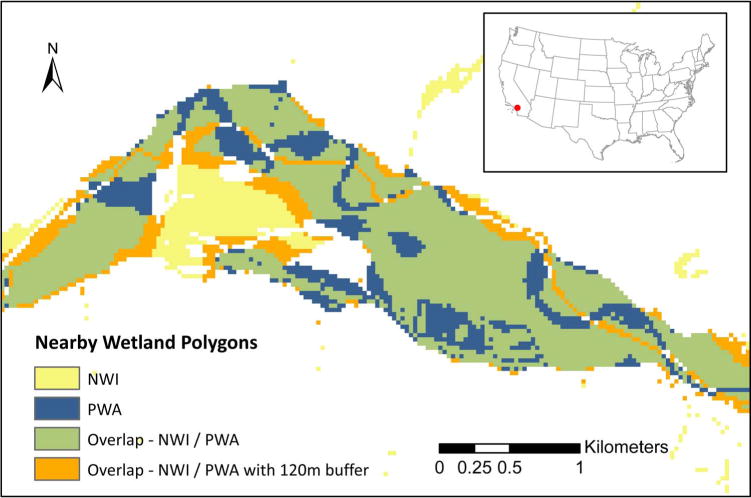
Close up of National Wetland Inventory (NWI) and potential wetland area (PWA) overlap in relation to nearby wetland polygons, demonstrating the potential for transitional differences between soil and wetland demarcations.
2.5. Potentially restorable wetlands on agricultural land
To create the PRW-Ag layer, we combined the PWA classes with LULC classes from the 2006 NLCD. LULC classes that were unlikely to be selected for wetland restoration, such as developed lands or large water bodies, were excluded from the selection. While wetland restoration can occur and provide benefits within other land use classes, such as open or low intensity development sites, these developed classes are also more likely to contain unsuitable land cover such as impervious surfaces and may also be more likely to be commercially valuable for other uses. In such cases, buffers may be a more suitable alternative to offset impacts to streams. It was assumed that natural land covers, such as forest, grassland, and existing wetlands, would not require extensive restoration. We, therefore, focused on agricultural land (pasture/hay [land cover code = 81] and cultivated crops [land cover code = 82]) in combination with the PWA classes.
3. Results
3.1. Topographic index and soil drainage
The CTI ≥ 550 layer selected 19–38% of the state’s land areas for all states except Florida where 76% of the state of Florida had CTI values ≥ 550 (Table 1). The percent of NWI emergent and forested overlapping the CTI ≥ 550 for the eleven test states ranged between 66% in Ohio and 92% in Florida (Table 1) with an overall intersection of 83%. Applying our CTI ≥ 550 across the CONUS resulted in close to 280 million ha or 37% of the land area being selected for our first layer in developing the PWA index (Fig. 3a).
Fig. 3.

Map of the spatial distribution of a) Compound Topographic Index (CTI ≥ 550), b) poorly drained and very poorly drained soils (PVP), c) combined indicator of potential wetland areas (PWA), and d) potentially restorable wetlands on agricultural land (PRW-Ag).
The presence of PVP soils was more varied across the eleven states than the CTI ≥ 550. The total area of PVP ranged from 6% in Washington and California to 76% in Mississippi (Table 1). These large differences in PVP may be the result of differences between state or even county level soil survey methodologies. When compared to NWI in our eleven states, we found that PVP alone accounts for a state average of 76% of the NWI wetland area. The lowest agreement was in the states of California and Washington where PVP intersected only 42% of NWI wetland areas. Across the entire CONUS, PVP included almost 195 million ha or 25% of the land area. The impact of the potential soil survey bias, both positive and negative, in the identification of PVP soils can be seen in the spatial distribution across the CONUS (Fig. 3b).
3.2. Potential wetland areas
Combining the CTI and PVP data layers resulted in a constrained extent for the PWA layer. In states where the amount of PVP was high, such as Mississippi (76% of state) or South Dakota (64% of the state), the CTI acted as a mask to reduce the PWA in those states (Fig. 3c). Similarly, in areas where CTI alone suggested a more extensive amount of wet areas, PVP constrained the selection to only those regions of PVP soils. The final PWA layer resulted in almost 120 million ha or 16% of the CONUS having wetland restoration potential. We found that the percentage of NWI emergent and forested wetlands overlap with the PWA classes (high, moderate, and low) ranged between 39 and 95% across the eleven states (Table 2). Together, the three PWA classes overlapped 81% of NWI for a total of 9.7 million ha. The high PWA class (CTI ≥ 550 and ≥ 80% PVP soils) had a greater percentage overlap with NWI in all states when compared to the low PWA and in nine out of the eleven states compared to the moderate PWA class. The high PWA class accounted for 59% of NWI hectares and ranged from 25% in Washington to 85% in Florida. The moderate PWA accounted for an additional 14% across the selected states while the low potential class contributed 8% to the total. In Washington, California and Ohio, overall capture of NWI by PWA was low (39%, 39%, and 51%). In these states, a greater number of NWI wetlands immediately adjacent to PWA were excluded as a result of a shift to CTI below 550 or to somewhat poorly drained soils. By including nearby NWI, within a buffer of 120 m, the overall agreement for these three states increased to more than 60%. We found that the excluded NWI wetlands were frequently classified as temporary and seasonal wetlands where water is only present for short periods of the year or were located in detailed riparian headwaters.
Table 2.
Area and percent of overlap between the National Wetland Inventory (NWI) and low, moderate and high indicators of potential wetland areas (PWA) across eleven states.
| Location | PWA within state (ha) | % of State Area | Low PWA Overlap with NWI (ha) | % NWI | Moderate PWA Overlap with NWI (ha) | % NWI | High PWA Overlap with NWI (ha) | % NWI | Total PWA Overlap with NWI (ha) | % NWI | PWA + 120 m Buffer Overlap with NWI (ha) | % NWI |
|---|---|---|---|---|---|---|---|---|---|---|---|---|
| CA | 1,537,949 | 4 | 11,934 | 2 | 51,885 | 9 | 164,644 | 28 | 228,463 | 39 | 348,636 | 60 |
| FL | 10,013,884 | 68 | 234,481 | 6 | 178,947 | 5 | 3,380,010 | 85 | 3,793,439 | 95 | 3,952,388 | 99 |
| GA | 4,102,227 | 27 | 130,456 | 7 | 310,399 | 16 | 1,197,922 | 63 | 1,638,776 | 86 | 1,865,712 | 98 |
| IA | 4,623,346 | 32 | 15,565 | 7 | 90,657 | 39 | 71,168 | 31 | 177,390 | 76 | 228,906 | 98 |
| MO | 3,667,931 | 20 | 31,521 | 8 | 110,702 | 27 | 119,705 | 29 | 261,927 | 64 | 392,475 | 95 |
| MS | 4,088,701 | 33 | 102,738 | 7 | 543,505 | 36 | 387,759 | 26 | 1,034,002 | 69 | 1,500,540 | 99 |
| NC | 3,971,905 | 31 | 256,841 | 17 | 116,524 | 8 | 972,969 | 65 | 1,346,334 | 90 | 1,488,391 | 99 |
| NY | 1,367,131 | 11 | 66,616 | 10 | 78,362 | 11 | 305,259 | 44 | 450,238 | 65 | 641,725 | 92 |
| OH | 2,228,368 | 21 | 22,010 | 11 | 7,242 | 4 | 75,522 | 37 | 104,774 | 51 | 168,311 | 82 |
| SD | 6,257,568 | 31 | 27,330 | 4 | 209,623 | 31 | 357,000 | 52 | 593,953 | 87 | 671,898 | 99 |
| WA | 484,725 | 3 | 17,210 | 7 | 21,752 | 8 | 64,887 | 25 | 103,850 | 39 | 174,223 | 66 |
3.3. Potentially restorable wetlands on agricultural land
The combination of PWA with the NLCD agricultural lands resulted in a total of over 46 million ha of agricultural land being selected as PRW-Ag across the CONUS (Fig. 3d). We found that watersheds having the highest percentage of PRW-Ag were clustered in bands throughout the Central Plains and Temperate Prairies (Fig. 4). Together these two ecoregions had over 22 million ha of PRW-Ag (Table 3). The Mississippi Alluvial and Southeast Coastal Plains and Texas-Louisiana Coastal Plain had the next highest total PRW-Ag with pockets of high potential PRW-Ag watersheds concentrated in southern Florida and along the Mississippi River. Additional watershed clusters of high potential PRW-Ag were found in the San Joaquin Valley of central California.
Fig. 4.

Percent of potentially restorable wetlands on agricultural land (PRW-Ag) within 12-digit hydrologic unit (HUC) watersheds across the contiguous U.S. (CONUS).
Table 3.
Hectares of agricultural land selected as potentially amenable to wetland restoration (PRW-Ag) across ecoregions by the three classes of wetland potential.
| Omernik Level 2 Ecoregion Name | Ecoregion Code | Low PRW-Ag (ha) | % Ecoregion | Moderate PRW-Ag (ha) | % Ecoregion | High PRW-Ag (ha) | % Ecoregion | Total PRW-Ag (ha) | % Ecoregion |
|---|---|---|---|---|---|---|---|---|---|
| Mixed Wood Shield | 5.2 | 38,576 | 0 | 134,285 | 1 | 247,983 | 1 | 420,844 | 2 |
| Atlantic Highlands | 5.3 | 38,674 | 0 | 43,075 | 0 | 28,938 | 0 | 110,687 | 1 |
| Western Cordillera | 6.2 | 43,456 | 0 | 220,083 | 0 | 262,957 | 0 | 526,495 | 1 |
| Marine West Coast Forest | 7.1 | 46,831 | 1 | 117,228 | 1 | 171,857 | 2 | 335,916 | 4 |
| Mixed Wood Plains | 8.1 | 536,895 | 1 | 633,077 | 2 | 1,324,509 | 3 | 2,494,480 | 7 |
| Central USA Plains | 8.2 | 878,950 | 4 | 1,272,934 | 6 | 4,418,555 | 20 | 6,570,438 | 29 |
| Southeastern USA Plains | 8.3 | 558,949 | 1 | 2,404,201 | 2 | 1,855,889 | 2 | 4,819,039 | 5 |
| Ozark/Ouachita-Appalachian Forests | 8.4 | 125,577 | 0 | 551,086 | 1 | 161,384 | 0 | 838,047 | 2 |
| Mississippi Alluvial & Southeast Coastal Plains | 8.5 | 573,257 | 2 | 1,455,116 | 4 | 4,470,921 | 13 | 6,499,294 | 20 |
| Temperate Prairies | 9.2 | 2,039,693 | 4 | 8,373,825 | 16 | 5,694,313 | 11 | 16,107,831 | 31 |
| West-Central Semiarid Prairies | 9.3 | 39,672 | 0 | 3,117,022 | 5 | 205,918 | 0 | 3,362,612 | 6 |
| South Central Semiarid Prairies | 9.4 | 15,312 | 0 | 1,437,067 | 1 | 122,952 | 0 | 1,575,331 | 2 |
| Texas-Louisiana Coastal Plain | 9.5 | 33,473 | 0 | 881,218 | 12 | 368,415 | 5 | 1,283,107 | 18 |
| Tamaulipas-Texas Semiarid Plain | 9.6 | 15 | 0 | 2,406 | 0 | 164 | 0 | 2,585 | 0 |
| Cold Deserts | 10.1 | 29,445 | 0 | 510,905 | 1 | 295,441 | 0 | 835,791 | 1 |
| Warm Deserts | 10.2 | 85 | 0 | 3,125 | 0 | 1,130 | 0 | 4,339 | 0 |
| Mediterranean California | 11.1 | 10,061 | 0 | 85,082 | 1 | 495,779 | 3 | 590,922 | 4 |
| Western Sierra Madre Piedmont | 12.1 | 0 | 0 | 61 | 0 | 0 | 0 | 61 | 0 |
| Upper Gila Mountains | 13.1 | 0 | 0 | 0 | 0 | 0 | 0 | 0 | 0 |
| Everglades | 15.4 | 16,669 | 1 | 20,943 | 1 | 277,026 | 13 | 314,638 | 15 |
| Total | – | 5,025,588 | 0.66 | 21,262,738 | 2.78 | 20,404,131 | 2.67 | 46,692,457 | 6.10 |
4. Discussion
Dahl (1990) estimated that between 85.4 and 89.5 million ha of wetlands were present pre-settlement, but were reduced to 41.8 million ha by the mid-1980s, a reduction of between 43.6 and 47.7 million ha of wetlands. We estimated the acreage of potentially restorable wetlands on agricultural land to be 46.7 million ha. The Central Plains and Temperate Prairies have sustained the greatest historical wetland losses. Dahl (1990) estimated that between 1790 and 1980 the Eastern Corn Belt (ECB) states lost between 85 and 90% of their historic wetlands as a result of conversion to agriculture. Drainage of wetlands accelerated in the 1850 through the early 1900s as subsurface tiling, advanced machinery, and government programs made drainage of wetlands more effective and affordable. Use of flexible plastic drainage lines and additional technologies allowed for additional drainage after World War II.
Given that conditions supporting wetlands are typically located in areas of low topographic relief and on poorly drained soils, our PRW-Ag was expected to align with lands having artificial drainage. The National Agricultural Statistics Service conducts a census of agricultural products and practices every 5 years and, in the 2012 census, reported on surface and subsurface drainage. We compared the percent PRW-Ag to state level census statistics for drained agricultural lands to explore the relationship between potentially restorable agriculture and drained lands (Fig. 5; USDA, 2013). Fig. 5 indicates that the states of Iowa, Illinois, Indiana, and Ohio had a higher percentage of drained agricultural lands than would be expected based on PRW-Ag. The relatively low cost of drainage installation and high yield returns on corn and soybeans would make draining even marginally wet areas economically feasible for farmers (e.g., somewhat poorly drained soils). However, while conversion of wetlands to drained agriculture in these four states has allowed for greater crop yields, it has also been linked to increased nutrient loads to water bodies. Numerous water quality studies have shown the impact of artificial drainage on nitrogen transport at both local (Dean and Foran, 1992; Randall et al., 2000; Cook and Baker, 2001; Randall and Goss, 2008; Cuadra and Vidon, 2011) and regional scales (Petrolina and Gowda, 2006; Royer et al., 2006; Alexander et al., 2007; David et al., 2010; Robertson et al., 2014; Smith et al., 2015). Landscape models of nutrient loading to the Gulf of Mexico indicate that between 25 and 29% of total nitrogen flux comes primarily from these four ECB states (Robertson et al., 2009).
Fig. 5.
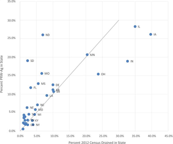
State level comparison between percent of artificially drained soils and potentially restorable wetlands on agricultural land (PRW-Ag). 1:1 line included for reference.
Unlike the ECB, the Dakotas have less artificial drainage than would be expected according to the PRW-Ag (Fig. 5). This difference may reflect the historically high evapotranspiration to precipitation ratios that exist in the Dakotas, past economic constraints, cultural differences, and more diversified agriculture such as wheat, sugar beet, sunflower, flax and more pasture land (USDA, 2015). As the region has more recently experienced wetter conditions, increased corn and soybean acreage, and increased crop prices, Minnesota and the Dakotas have seen a rise in drained landscapes (Sands et al., 2010; Snider, 2015). The Dakotas contribute a smaller proportion of the total nutrient load to the Mississippi River (Alexander et al., 2007), which seems to be reflected in the ratio of drained agricultural land to potentially restorable wetlands in these two states. The PRW-Ag indicated that states in the Central Plains and Temperate Prairies had a higher potential for wetland restoration, such as the glaciated Des Moines Lobe in North Central Iowa and Southern Minnesota, as well as the glaciated plains of South Dakota and up through the Red River Valley of North Dakota and Minnesota (Fig. 4).
4.1. Potential applications
Our PWA and PRW-Ag layers were developed to enhance and assist coordination and prioritization efforts to identify and restore landscapes that support wetlands. The PWA and PRW-Ag layers can be used to identify, in a spatially explicit manner, potential sites for restoration of a particular type of service. For example, if water quality is the main focus, finding restorable sites downstream from polluted headwaters might be of interest. In the 1850s, the Great Black Swamp (GBS) in northwest Ohio covered 400,000 ha, but was subsequently drained and is now dominated by row crop agriculture and livestock production (Herdendorf, 1992, http://www.blackswamp.org/). Lake Erie and smaller lakes within the northwest Ohio region routinely suffer from algal blooms. These blooms limit recreation and can affect drinking water supplies (e.g., Toledo, OH in 2014), and are in part due to agricultural nutrient loads in the Lake Erie basin (Michalak et al., 2013; Paerl et al., 2014). Federal and state agencies are encouraging nutrient management plans for Lake Erie and the GBS for fertilizer reductions and adoption of best management practices, including wetland restoration (Ohio Department of Agriculture, 2013). Within northeast Ohio, our PRW-Ag layer highlights concentrated potentially restorable wetland areas within the GBS that could inform multiple private and state entities that are in the process of restoring marginal lands within the GBS (Fig. 3d; http://www.blackswamp.org/; https://www.glri.us/projects/epa.html). In Iowa, a nutrient reduction initiative encourages the prioritization of watersheds and specifically includes targeted wetland restorations as a conservation practice (IDALS et al., 2012). The Iowa Conservation Reserve Enhancement Program, in partnership with the USDA Farm Service Agency, had 95 wetlands constructed or planned, as of January 2014, to be placed strategically within the landscape to receive nutrient-rich waters and remove nitrate via denitrification (IDALS, 2014).
For restoration focused on habitat for waterfowl or other species, large areas of moderate or high potentially restorable lands near existing wetlands or other natural habitats can be identified within the PRW-Ag data layer (Fig. 3d). Numerous restoration and construction efforts have already begun in the agricultural Midwest, targeting wetland restoration for waterfowl habitat. These restorations often breach the local field tile lines at the wetland site in order to restore the wetland hydrology and allow wetland plants to recolonize the site (Galatowitsch and van der Valk, 1996). For example, Ducks Unlimited has restored more than 32,000 ha of waterfowl habitat across the U.S. with 8,400 ha in the Prairie Pothole Region of the U.S. and Canada in 2014 alone (Ducks Unlimited, 2015). This is a region where large percentages of PRW-Ag exist, which could help identify locations for additional adjacent restoration efforts.
Wetland losses in the bottom hardwood swamps of the Mississippi Alluvial Valley (MAV) have reduced a floodplain network of 10 million ha to 25% of its original size (Schoenholtz et al., 2001). Much of this conversion was made possible through river channelization, flood levees, and artificial drainage. Ecosystem services relating to sediment and nutrient retention, temporary flood abatement, carbon storage, and wildlife habitat were lost or degraded as a result. While restoration in the Upper Midwest can often restore hydrology through the relatively simple process of removing or “plugging” artificial drainage systems under the acreage to be restored, the challenges of wetland restoration in the MAV are different and complex. The bottomland wetlands of the MAV typically rely on natural flood-pulse cycles to provide water, nutrients, and sediments. Due to river channelization and levees, the ability to adequately restore natural hydrology is a complex task that requires coordination beyond the level of an individual farmer (Faulkner et al., 2011). The PRW-Ag layer identified over 4 million ha of high wetland restoration potential in the Mississippi Alluvial & Southeast Coastal Plains (Table 2). The Lower Mississippi Valley Joint Venture was created to coordinate and focus private and government funding and waterfowl restoration efforts in the Mississippi Alluvial and Southeast Coastal Plains. Together these initiatives have enhanced or restored from 102,000 to 160,000 ha of wetlands within the MAV (Faulkner et al., 2011; http://www.ducks.org/conservation/public-policy/wrp-helping-to-restore-bottomland-hardwoods-in-the-mississippi-alluvial-valley) and our PWA and PRW-Ag layers could help identify and inform ongoing restoration efforts.
4.2. Limitations
The PWA and PRW-Ag layers are constrained by the accuracy of the layers used to create them – namely the soils datasets, NED, CTI, NWI, and NLCD. The PVP layer is the result of the compilation of soils survey data over time, much of which was collected from the 1950s through the 1980s. Since the soils data was originally collected by and for agricultural land use and conservation, soil data was not usually collected for developed areas or for non-agricultural montane areas. For those areas where SSURGO was not available, the much coarser STATSGO2 layer was used which could introduce error for those regions (Appendix A). Additionally, soil classification can be subject to surveyor and boundary/definitional biases (such as the designation of poorly drained or somewhat poorly drained soil) as is evident from clear soil demarcations at state and county lines (e.g., Alabama and Georgia in Fig. 3b). The CTI data layer also has limitations including a 30 m grid size that will mask variation in microtopography and cannot be expected to accurately identify wet areas on its own without the consideration of precipitation/evaporation. Alone, the CTI classified large areas of the arid Southwest as potentially wet and were only excluded from the PWA and PRW-Ag because of the inclusion of the PVP layer and/or the mask of agricultural land use. In addition, using a digital elevation algorithm such as CTI, rarer wetland types such as fens could be missed as they are not found in topographic depressions. (Rampi et al., 2014).
There were several states, notably California, Washington, and Ohio, where the combined PWA layer missed detecting 18-40% of the NWI wetlands, even with a 120 m buffer. Some of the discrepancy likely arises from the differing resolution of the NWI maps and the soil layers. The scale of the NWI data ranges from better than 1:40,000 (with a minimum mapping unit typically around 0.4 ha) to over 1:80,000 (with a minimum mapping unit of 1–2 ha) (Appendix B; USFWS, 2016), which aligns well with the SSURGO field surveys delineated soil map units from 0.4 to 4.0 ha in size, but only has marginal alignment with the STATSGO2 soil map units of approximately 1,000 ha. Some NWI wetlands in Washington were montane riparian areas located in regions with only STATSGO2 soils data available (Appendix A). Likewise, soil surveyors in California and Ohio were more prone to use the “somewhat poorly drained” classification for areas than other states. Additionally, PWA comparisons with NWI occurred as a grid cell by grid cell comparison so while the center of an NWI wetland might have overlapped with our PWA designation, the edges of the NWI polygon might have remained outside of the PWA and were considered as non-overlapping in the analysis. Similarly, small or narrow NWI features may not have aligned enough with a cell center to designate the cell as a NWI wetland, also resulting as non-overlapping in the analysis. Overall, the PWA and PRW-Ag provide useful information for the spatial identification of potential wetland restoration, but the underlying assumptions and limitations need to be taken into account when using the datasets in decision-making.
5. Conclusions
The PWA and PRW-Ag layers provide useful information to assist agencies and private organizations in identifying areas of potential wetland restoration. By providing the PWA and PRW-Ag layers for the CONUS, decision makers can leverage the increased benefits of planning across a watershed or multiple watersheds. The PWA combines the topographic index and soil drainage layers, but does not filter by land cover type, allowing decision makers to incorporate their own land cover types as applicable. The PRW-Ag incorporates agricultural and pasture lands into the PWA as a filter for lands most likely to be amenable to wetland restoration. While our data layers are less likely to catch more ephemeral wetland areas where soils have higher drainage, they do provide a good approximation of locations for successful establishment of perennial wetlands. The PWA and PRW-Ag layers provide a solid basis to begin planning. When combined with field analyses and verification, they have the potential to help facilitate needed wetland restoration efforts.
Our PWA and PRW-Ag layers are currently available in the EnviroAtlas (https://www.epa.gov/enviroatlas) where they can be combined with other available layers, such as land cover within riparian buffers, synthetic nitrogen fertilizer application, impaired waters, rare ecosystems, and protected lands (Fig. 6; Pickard et al., 2015). The PWA and PRW-Ag grids can also be downloaded by the user for use with other data and tools that have been designed to provide guidance on wetland placement (e.g., http://www.eli.org/freshwater-ocean/tools-evaluating-feasibility-restoration). By providing these data for download and use in a publically available mapping application, we give decision makers the flexibility of placing potential wetlands in the context of regional or organization goals, ongoing efforts, ecosystem markets, and prioritization of further analyses.
Fig. 6.

Screen capture of EPA’s EnviroAtlas web application (https://www.epa.gov/enviroatlas) showing potentially restorable wetlands on agricultural land (PRW-Ag) layers and other supplementary data related to stream conditions and ecosystem services.
Supplementary Material
Acknowledgments
This project was supported in part by an appointment to the Research Participation Program for the U.S. Environmental Protection Agency, Office of Research and Development, administered by the Oak Ridge Institute for Science and Education through an interagency agreement between the U.S. Department of Energy and EPA. The views expressed in this article are those of the authors and do not necessarily reflect the views or policies of the EPA.
Appendix A. SSURGO and STATSGO2
Fig. A1.

Geographic (SSURGO) and the State Soil Geographic (STATSGO2) database (Soil Survey Staff, 2006a,b). Where available, the more detailed SSURGO, with a spatial scale ranging from 1:12k to 1:64k, was used. Where SSURGO was unavailable (i.e., mountains, deserts, and military land), STATSGO2 data was used with an aggregated spatial scale of 1:250k.
Appendix B. NWI
Table B1.
National Wetlands Inventory (NWI) collection date, scale, area and percent wetland type for selected states.
| State | Imagery Date | Scale | Wetlands (ha) | Percent Freshwater Emergent Wetland | Percent Freshwater Forested/Shrub Wetland | Percent Freshwater Pond | Percent Lake | Percent Other (except Estuarine and Marine Deepwater) |
|---|---|---|---|---|---|---|---|---|
| CA | 1970s-2000s | 1:40k-1:80k | 708,532 | 24 | 9 | 2 | 43 | 22 |
| FL | 1970s-2000s | 1:40k-1:80k | 2,057,514 | 26 | 52 | 2 | 10 | 10 |
| GA | 1970s-2000s | 1:40k-1:58k | 931,997 | 4 | 78 | 4 | 6 | 8 |
| IA | 1980s-2000s | 1:40k | 167,077 | 20 | 36 | 11 | 16 | 17 |
| MO | 1980s-2000s | 1:58k | 300,374 | 14 | 41 | 14 | 17 | 13 |
| MS | 1970s-2000s | 1:40k-1:80k | 731,209 | 3 | 80 | 4 | 6 | 6 |
| NC | 1980s-2000s | 1:40k-1:58k | 724,658 | 3 | 81 | 3 | 7 | 7 |
| NY | 1970s-2000s | 1:40k-1:80k | 452,361 | 10 | 53 | 5 | 27 | 6 |
| OH | 2000s | 1:40k | 148,194 | 12 | 44 | 15 | 18 | 10 |
| SD | 1970s-1980s | 1:58k-1:80k | 424,041 | 63 | 2 | 7 | 25 | 3 |
| WA | 1970s-2000s | 1:40k-1:80k | 241,363 | 23 | 21 | 3 | 40 | 12 |
Appendix C. Supplementary data
Supplementary data associated with this article can be found, in the online version, at http://dx.doi.org/10.1016/j.ecolind.2017.07.026.
References
- Adusumilli N. Valuation of ecosystem services from wetlands mitigation in the United States. Land. 2015;4(1):182–196. http://dx.doi.org/10.3390/land4010182. [Google Scholar]
- Alexander RB, Smith RA, Schwarz GE, Boyer EW, Nolan JV, Brakebill JW. Differences in phosphorus and nitrogen delivery to the Gulf of Mexico from the Mississippi River Basin. Environ Sci Technol. 2007;42(3):822–830. doi: 10.1021/es0716103. http://dx.doi.org/10.1021/es0716103. [DOI] [PubMed] [Google Scholar]
- Beven KJ, Kirkby MJ. A physically based, variable contributing area model of basin hydrology/Un modèle à base physique de zone d’appel variable de l’hydrologie du bassin versant. Hydrol Sci J. 1979;24(1):43–69. http://dx.doi.org/10.1080/02626667909491834. [Google Scholar]
- Bowen MW, Johnson WC, Egbert SL, Klopfenstein ST. A GIS-based approach to identify and map playa wetlands on the High Plains, Kansas, USA. Wetlands. 2010;30(4):675–684. http://dx.doi.org/10.1007/s13157-010-0077-z. [Google Scholar]
- Caldwell PV, Vepraskas MJ, Gregory JD, Skaggs RW, Huffman RL. Linking plant ecology and long-term hydrology to improve wetland restoration success. Trans ASABE. 2011;54(6):2129–2137. http://dx.doi.org/10.13031/2013.40662. [Google Scholar]
- Cook MJ, Baker JL. Bacteria and nutrient transport to the tile lines shortly after application of large volumes of liquid swine manure. Trans ASAE. 2001;44(3):495. http://dx.doi.org/10.13031/2013.6109. [Google Scholar]
- Cowardin LM, Carter V, Golet FC, LaRoe ET. Classification of Wetlands and Deepwater Habitats of the United States. U.S. Department of the Interior, U.S. Fish and Wildlife Service; 1979. [Google Scholar]
- Creed IF, Sass GZ. Forest Hydrology and Biogeochemistry. Springer; Netherlands: 2011. Digital terrain analysis approaches for tracking hydrological and biogeochemical pathways and processes in forested landscapes; pp. 69–100. http://dx.doi.org/10.1007/978-94-007-1363-5_4. [Google Scholar]
- Crumpton WG, Stenback GA, Miller BA, Helmers M. Potential benefits of wetland filters for tile drainage systems: Impact on nitrate loads to Mississippi River Subbasins. Ecology, Evolution and Organismal Biology Reports. 2006;2 http://lib.dr.iastate.edu/eeob_ag_reports/2. [Google Scholar]
- Cuadra PE, Vidon P. Storm nitrogen dynamics in tile-drain flow in the US Midwest. Biogeochemistry. 2011;104(1–3):293–308. http://dx.doi.org/10.1007/s10533-010-9502-x. [Google Scholar]
- Curie F, Gaillard S, Ducharne A, Bendjoudi H. Geomorphological methods to characterise wetlands at the scale of the Seine watershed. Sci Total Environ. 2007;375(1):59–68. doi: 10.1016/j.scitotenv.2006.12.013. http://dx.doi.org/10.1016/j.scitotenv.2006.12.013. [DOI] [PubMed] [Google Scholar]
- Dahl TE, Johnson CE. Status and Trends of Wetlands in the Conterminous United States, Mid-1970s to Mid-1980s. U.S. Department of the Interior, Fish and Wildlife Service; Washington, DC: 1991. p. 28. [Google Scholar]
- Dahl TE. Report to the Congress. National Wetlands Inventory; St. Petersburg, FL, USA No. PB-91-169284/XAB: 1990. Wetlands Losses in the United States, 1780’s to 1980’s. [Google Scholar]
- Dahl TE. Status and Trends of Wetlands in the Conterminous United States 2004 to 2009. U.S. Department of the Interior, Fish and Wildlife Service, Fisheries and Habitat Conservation; 2011. [Google Scholar]
- David MB, Drinkwater LE, McIsaac GF. Sources of nitrate yields in the Mississippi River Basin. J Environ Qual. 2010;39(5):1657–1667. doi: 10.2134/jeq2010.0115. http://dx.doi.org/10.2134/jeq2010.0115. [DOI] [PubMed] [Google Scholar]
- Dean DM, Foran ME. The effect of farm liquid waste application on tile drainage. J Soil Water Conserv. 1992;47(5):368–369. [Google Scholar]
- Diebel MW, Maxted JT, Nowak PJ, Van der Zanden MJ. Landscape planning for agricultural nonpoint source pollution reduction I: a geographical allocation framework. Environ Manage. 2008;42(5):789–802. doi: 10.1007/s00267-008-9186-3. http://dx.doi.org/10.1007/s00267-008-9186-3. [DOI] [PubMed] [Google Scholar]
- Ducks Unlimited. Ducks Unlimited Fact Sheet. 2015 http://www.ducks.org/media/_global/_documents/stateFactSheets/NationalFactSheet.pdf (Accessed 11/2015)
- Faulkner S, Barrow W, Jr, Keeland B, Walls S, Telesco D. Effects of conservation practices on wetland ecosystem services in the Mississippi Alluvial Valley. Ecol Appl. 2011;21:S31–S48. http://dx.doi.org/10.1890/10-0592.1. [Google Scholar]
- Fry J, Xian G, Jin S, Dewitz J, Homer C, Yang L, Barnes C, Herold N, Wickham J. Completion of the 2006 National Land Cover Database for the Conterminous United States. PE&RS. 2011;77(9):858–864. [Google Scholar]
- Galatowitsch SM, van der Valk AG. Characteristics of recently restored wetlands in the prairie pothole region. Wetlands. 1996;16(1):75–83. http://dx.doi.org/10.1007/BF03160647. [Google Scholar]
- Hansen L, Hellerstein D. Better Targeting, Better Outcomes. U.S. Department of Agriculture, Economic Research Service; 2006. [Google Scholar]
- Herdendorf CE. Lake Erie coastal wetlands: an overview. J Great Lakes Res. 1992;18(4):533–551. http://dx.doi.org/10.1016/S0380-1330(92)71321-5. [Google Scholar]
- Iowa Department of Agriculture and Land Stewardship (IDALS), Iowa Department of Natural Resources, Iowa State University College of Agriculture and Life Sciences. Iowa Nutrient Reduction Strategy: A Science and Technology-based Framework to Assess and Reduce Nutrients to Iowa Waters and the Gulf of Mexico. Iowa State University College of Agriculture and Life Sciences; Ames, IA: 2012. http://www.nutrientstrategy.iastate.edu/sites/default/files/documents/NRSfull.pdf (Accessed 11/2015) [Google Scholar]
- Iowa Department of Agriculture and Land Stewardship. Iowa Conservation Reserve Enhancement Program: 2014 Annual Performance Report. 2014 http://www.iowaagriculture.gov/waterresources/pdf/2014/crep/2014IowaCREPAnnualReport.pdf (Accessed 11/2015)
- Kayranli B, Scholz M, Mustafa A, Hedmark Å. Carbon storage and fluxes within freshwater wetlands: a critical review. Wetlands. 2010;30(1):111–124. http://dx.doi.org/10.1007/s13157-009-0003-4. [Google Scholar]
- Lang M, McCarty G, Oesterling R, Yeo IY. Topographic metrics for improved mapping of forested wetlands. Wetlands. 2013;33(1):141–155. http://dx.doi.org/10.1007/s13157-012-0359-8. [Google Scholar]
- Millennium Ecosystem Assessment (MEA) Ecosystems and Human Well-being: Wetlands and Water Synthesis. World Resources Institute; Washington, D.C.: 2005. [Google Scholar]
- McCauley LA, Jenkins DG. GIS-based estimates of former and current depressional wetlands in an agricultural landscape. Ecol Appl. 2005;15(4):1199–1208. http://dx.doi.org/10.1890/04-0647. [Google Scholar]
- Michalak AM, Anderson EJ, Beletsky D, Boland S, Bosch NS, Bridgeman TB, Chaffin JD, Cho K, Confesor R, Daloğlu I, DePinto JV. Record-setting algal bloom in Lake Erie caused by agricultural and meteorological trends consistent with expected future conditions. Proc Natl Acad Sci U S A. 2013;110(16):6448–6452. doi: 10.1073/pnas.1216006110. http://dx.doi.org/10.1073/pnas.1216006110. [DOI] [PMC free article] [PubMed] [Google Scholar]
- Mitsch WJ, Hernandez ME. Landscape and climate change threats to wetlands of North and Central America. Aquat Sci. 2013;75(1):133–149. http://dx.doi.org/10.1007/s00027-012-0262-7. [Google Scholar]
- Moreno-Mateos D, Comín FA. Integrating objectives and scales for planning and implementing wetland restoration and creation in agricultural landscapes. J Environ Manage. 2010;91(11):2087–2095. doi: 10.1016/j.jenvman.2010.06.002. http://dx.doi.org/10.1016/j.jenvman.2010.06.002. [DOI] [PubMed] [Google Scholar]
- National Research Council. Compensating for Wetland Losses Under the Clean Water Act. The National Academies Press; Washington, DC: 2001. [Google Scholar]
- Natural Resources Conservation Service (NRCS) Restoring America’s Wetlands: A Private Lands Conservation Success Story. United States Department of Agriculture, Wetlands Reserve Program; 2012. http://www.nrcs.usda.gov/Internet/FSE_DOCUMENTS/stelprdb1045079.pdf (Accessed 11/2015) [Google Scholar]
- Ohio Department of Agriculture. Ohio Lake Erie Phosphorus Task Force II Final Report. Ohio Department of Agriculture; Columbus, OH: 2013. http://www.epa.ohio.gov/portals/35/lakeerie/ptaskforce2/Task_Force_Report_October_2013.pdf (Accessed 12 August 2016) [Google Scholar]
- Paerl HW, Gardner WS, McCarthy MJ, Peierls BL, Wilhelm SW. Algal blooms: noteworthy nitrogen. Science. 2014;346(6206):175. doi: 10.1126/science.346.6206.175-a. [DOI] [PubMed] [Google Scholar]
- Palmer MA. Reforming watershed restoration: science in need of application and applications in need of science. Estuaries Coasts. 2009;32(1):1–17. [Google Scholar]
- Petrolina DR, Gowda PH. Missing the boat: midwest farm drainage and the Gulf of Mexico hypoxia. Appl Econ Perspect Policy. 2006;28(2):240–253. http://dx.doi.org/10.1111/j.1467-9353.2006.00284.x. [Google Scholar]
- Pickard BR, Daniel J, Mehaffey M, Jackson LE, Neale A. EnviroAtlas: a new geospatial tool to foster ecosystem services science and resource management. Ecosyst Serv. 2015;14:45–55. http://dx.doi.org/10.1016/j.ecoser.2015.04.005. [Google Scholar]
- Rampi LP, Knight JF, Lenhart CF. Comparison of flow direction algorithms in the application of the CTI for mapping wetlands in Minnesota. Wetlands. 2014;34(3):513–525. http://dx.doi.org/10.1007/s13157-014-0517-2. [Google Scholar]
- Randall GW, Goss MJ. Nitrate Losses to Surface Water Through Subsurface, Tile Drainage Nitrogen in the Environment: Sources, Problems, and Management. 2nd. Elsevier; New York: 2008. pp. 145–175. [Google Scholar]
- Randall GW, Iragavarapu TK, Schmitt MA. Nutrient losses in subsurface drainage water from dairy manure and urea applied for corn. J Environ Qual. 2000;29:1244–1252. http://dx.doi.org/10.2134/jeq2000.00472425002900040031x. [Google Scholar]
- Robertson DM, Schwarz GE, Saad DA, Alexander RB. Incorporating uncertainty into the ranking of SPARROW model nutrient yields from Mississippi/Atchafalaya river basin watersheds. JAWRA J Am Water Resour Assoc. 2009;45(2):534–549. doi: 10.1111/j.1752-1688.2009.00310.x. http://dx.doi.org/10.1111/j.1752-1688.2009.00310.x. [DOI] [PMC free article] [PubMed] [Google Scholar]
- Robertson DM, Saad DA, Schwarz GE. Spatial variability in nutrient transport by HUC8, state, and subbasin based on Mississippi/Atchafalaya river basin SPARROW models. JAWRA J Am Water Resour Assoc. 2014;50(4):988–1009. http://dx.doi.org/10.1111/jawr.12153. [Google Scholar]
- Rosenblatt AE, Gold AJ, Stolt MH, Groffman PM, Kellogg DQ. Identifying riparian sinks for watershed nitrate using soil surveys. J Environ Qual. 2001;30(5):1596–1604. doi: 10.2134/jeq2001.3051596x. http://dx.doi.org/10.2134/jeq2001.3051596x. [DOI] [PubMed] [Google Scholar]
- Royer TV, David MB, Gentry LE. Timing of riverine export of nitrate and phosphorus from agricultural watersheds in Illinois: implications for reducing nutrient loading to the Mississippi river. Environ Sci Technol. 2006;40:4126–4131. doi: 10.1021/es052573n. http://dx.doi.org/10.1021/es052573n. [DOI] [PubMed] [Google Scholar]
- Sands GR, Kandel H, Hay C, Scherer T. University of Minnesota Extension: Frequently Asked Questions about Subsurface (Tile) Drainage in the Red River Valley. 2010 http://www.extension.umn.edu/agriculture/water/publications/pdfs/faqs_of_tile_drainageprint_61313.pdf (Accessed 11/2015)
- Schoenholtz SH, James JP, Kaminski RM, Leopold BD, Ezell AW. Afforestation of bottomland hardwoods in the Lower Mississippi Alluvial Valley: status and trends. Wetlands. 2001;21(4):602–613. http://dx.doi.org/10.1672/0277-5212(2001)021[0602:AOBHIT]2.0.CO;2. [Google Scholar]
- Schuyt K, Brander L. Living Waters Conserving the Source of Life: the Economic Values of the World’s Wetlands. World Wildlife Fund; Gland/Amsterdam, Netherlands: 2004. [Google Scholar]
- Smith DR, King KW, Johnson L, Francesconi W, Richards P, Baker D, Sharpley AN. Surface runoff and tile drainage transport of phosphorus in the mid-western United States. J Environ Qual. 2015;44(2):495–502. doi: 10.2134/jeq2014.04.0176. http://dx.doi.org/10.2134/jeq2014.04.0176. [DOI] [PubMed] [Google Scholar]
- Snider A. WATER POLICY: weather, farm bill programs turn North Dakotans against obama rule. Environment and Energy Daily. 2015 Published: 15 May 2015. [Google Scholar]
- Soil Survey Staff, Natural Resources Conservation Service (NRCS), United States Department of Agriculture. Soil Survey Geographic (SSURGO) Database for [Survey Area, State] 2006a Available online (Accessed 01 February 2012) [Google Scholar]
- Soil Survey Staff, Natural Resources Conservation Service (NRCS), United States Department of Agriculture. U.S. General Soil Map (STATSGO2) 2006b Available online (Accessed 01 March 2012) [Google Scholar]
- Soil Survey Staff. Soil survey manual Soil conservation service. U.S. Gov. Print. Office; Washington, DC: 1993. (U.S. Department of Agriculture Handbook No. 18). [Google Scholar]
- Soil Survey Staff, Natural Resources Conservation Services (NRCS) Gridded Soil Survey Geographic (SSURGO) Database for the United States of American and the Territories, Commonwealths and Island Nations Served by the USDA NRCS. 2012 https://gdg.sc.egov.usda.gov/ (Accessed 23 January 2016)
- Tiner RW. Wetland Indicators: A Guide to Wetland Identification, Delineation, Classification, and Mapping. CRC Press; 1999. p. 424. (Technology & Engineering). April 21, 1999. [Google Scholar]
- U.S. Army Corps of Engineers (USACE) (Wetlands Research Program Technical Report Y-87-1).Corps of Engineers Wetlands Delineation Manual. 1987 http://www.fws.gov/habitatconservation/delineation%2087.pdf (Accessed 11/2015)
- U.S. Department of Agriculture (USDA) 2012 Census of Agriculture. USDA-National Agricultural Statistics Service; Washington, DC: 2013. https://www.agcensus.usda.gov/Publications/2012 (Accessed 08/2013) [Google Scholar]
- U.S. Department of Agriculture (USDA) 2007 National Crop Data Layer. USDA- National Agricultural Statistics Service; Washington, DC: 2015. http://nassgeodata.gmu.edu/CropScape/ (Accessed 11/2015) [Google Scholar]
- U. S. Fish and Wildlife Service (USFWS) National Wetlands Inventory. U.S. Department of the Interior, Fish and Wildlife Service; Washington, D.C.: 2016. https://www.fws.gov/wetlands/Data/Metadata.html (Accessed 20 July 2016) [Google Scholar]
- White D, Fennessy S. Modeling the suitability of wetland restoration potential at the watershed scale. Ecol Eng. 2005;24(4):359–377. http://dx.doi.org/10.1016/ecoleng.2005.01.012. [Google Scholar]
- Zedler JB. Progress in wetland restoration ecology. Trends Ecol Evol. 2000;15(10):402–407. doi: 10.1016/s0169-5347(00)01959-5. http://dx.doi.org/10.1016/S0169-5347(00)01959-5. [DOI] [PubMed] [Google Scholar]
- Zedler JB. Wetlands at your service: reducing impacts of agriculture at the watershed scale. Front Ecol Environ. 2003;1(2):65–72. http://dx.doi.org/10.1890/1540-9295(2003)001[0065:WAYSRI]2.0.C0;2. [Google Scholar]
Associated Data
This section collects any data citations, data availability statements, or supplementary materials included in this article.