Estimating Individual Treatment Effect in Observational Data Using Random Forest Methods

Abstract

Estimation of individual treatment effect in observational data is complicated due to the challenges of confounding and selection bias. A useful inferential framework to address this is the counterfactual (potential outcomes) model, which takes the hypothetical stance of asking what if an individual had received both treatments. Making use of random forests (RF) within the counterfactual framework we estimate individual treatment effects by directly modeling the response. We find that accurate estimation of individual treatment effects is possible even in complex heterogenous settings but that the type of RF approach plays an important role in accuracy. Methods designed to be adaptive to confounding, when used in parallel with out-of-sample estimation, do best. One method found to be especially promising is counterfactual synthetic forests. We illustrate this new methodology by applying it to a large comparative effectiveness trial, Project Aware, to explore the role drug use plays in sexual risk. The analysis reveals important connections between risky behavior, drug usage, and sexual risk.

1. Introduction

Even for a medical discipline steeped in a tradition of randomized trials, the evidence basis for only a few guidelines is based on randomized trials (Tricoci et al. 2009). In part this is due to continued development of treatments, in part to enormous expense of clinical trials, and in large part to the hundreds of treatments and their nuances involved in real-world, heterogenous clinical practice. Thus, many therapeutic decisions are based on observational studies. However, comparative treatment effectiveness studies of observational data suffer from two major problems: only partial overlap of treatments and selection bias. Each treatment is to a degree bounded within constraints of indication and appropriateness. Thus, transplantation is constrained by variables such as age, a mitral valve procedure is constrained by presence of mitral valve regurgitation. However, these boundaries overlap widely, and the same patient may be treated differently by different physicians or different hospitals, often without explicit or evident reasons. Thus, a fundamental hurdle in observational studies evaluating comparative effectiveness of treatment options is to address the resulting selection bias or confounding. Naively evaluating differences in outcomes without doing so leads to biased results and flawed scientific conclusions.

Formally, let {(X₁, T₁,Y₁), …, (X_n, T_n,Y_n)} denote the data where X_i is the covariate vector for individual i and Y_i is the observed outcome. Here T_i denotes the treatment group of i. For concreteness, let us say T_i = 0 represents the control group, and T_i = 1 the intervention group. Our goal is to estimate the individual treatment effect (ITE), defined as the difference in the mean outcome for an individual under both treatments, conditional on the observed covariates. More formally, let Y_i(0) amd Y_i(1) denote the potential outcome for i under treatments T_i = 0 and T_i = 1, respectively. Given X_i = x, the ITE for i is defined as the conditional mean difference in potential outcomes

$$\tau (\mathbf{x})=\mathbb{E}[Y_i(1)|{\mathbf{X}}_i=\mathbf{x}]-\mathbb{E}[Y_i(0)|{\mathbf{X}}_i=\mathbf{x}].$$ (1)

Definition (1) relies on what is called the counterfactual framework, or potential outcomes model (Rubin 1974; Neyman et al. 1990). In this framework, one plays the game of hypothesizing what would have happened if an individual i had received both treatments. However, the difficulty with estimating (1) is that although potential outcomes {Y_i(0),Y_i(1)} are hypothesized to exist, only the outcome Y_i from the actual treatment assignment is observed. Without additional assumptions, it is not possible in general to estimate (1). A widely used assumption to resolve this problem, and one that we adopt, is the assumption of strongly ignorable treatment assignment (SITA). This assumes that treatment assignment is conditionally independent of the potential outcomes given the variables, that is, T ⊥ {Y (0),Y (1)} | X. Under the assumption of SITA, we have

$$\begin{gathered} \tau (\mathbf{x})=\mathbb{E}[Y(1)|\mathbf{X}=\mathbf{x}]-\mathbb{E}[Y(0)|\mathbf{X}=\mathbf{x}] \\ =\mathbb{E}[Y(1)|T=1,\mathbf{X}=\mathbf{x}]-\mathbb{E}[Y(0)|T=0,\mathbf{X}=\mathbf{x}] \\ =\mathbb{E}[Y|T=1,\mathbf{X}=\mathbf{x}]-\mathbb{E}[Y|T=0,\mathbf{X}=\mathbf{x}]. \end{gathered}$$ (2)

Notice that the last expression involves conditional expectations of only observable values, thus making it possible to estimate τ (x). It should be emphasized that without SITA one cannot guarantee estimability of τ (x) in general because $\mathbb{E}[Y|T=j,\mathbf{X}=\mathbf{x}]=\mathbb{E}[Y(j)|\mathbf{X}=\mathbf{x}]$ does not always hold.

Typically, causal inference focuses on the estimation of the average treatment effect (ATE), a standard measure of performance in nonheterogenous treatment settings. The ATE is defined as

$$\begin{gathered} {\tau }_0=\mathbb{E}[Y(1)-Y(0)]-\mathbb{E}\{\mathbb{E}[Y(1)|\mathbf{X}=\mathbf{x}]-\mathbb{E}[Y(0)|\mathbf{X}=\mathbf{x}]\} \\ =\mathbb{E}[\tau (\mathbf{X})]. \end{gathered}$$ (3)

Although direct estimation of (3) under SITA is possible by using mean treatment differences in cells with the same X, due to the curse of dimensionality this method only works when X is low dimensional. Propensity score analysis (Rosenbaum and Rubin 1983) is one means to overcome this problem. The propensity score is defined as the conditional probability of receiving the intervention given X = x, denoted here by $e(\mathbf{x})=\mathrm{\mathbb{P}}\{T=1|\mathbf{X}=\mathbf{x}\}$. Under the assumption of SITA, the propensity score possesses the so-called balancing property. This means that T and X are conditionally independent given e(X). Thus, variables X are balanced between the two treatment groups after conditioning on the propensity score, thereby approximating a randomized clinical trial (Rubin 2007). Importantly, the propensity score is the coarsest possible balancing score, thus not only does it balance the data, but it does so by using the coarsest possible conditioning, thus helping to mitigate the curse of dimensionality. To use the propensity score for treatment effect estimation, Rosenbaum and Rubin (1983) further showed if SITA holds (which includes the assumption that the propensity score is bounded 0 < e(X) < 1), then treatment assignment is conditionally independent of the potential outcomes given the propensity score, that is, T ⊥ {Y (0),Y (1)} | e(X). This result is the foundation for ATE estimators based on stratification or matching of the data on propensity scores. However, this is not the only means for using the propensity score to estimate treatment effect. Another approach is to use SITA to derive weighted estimators for the ATE. Analogous to (2), under SITA one has

$$\begin{gathered} \mathbb{E}\left[\frac{TY}{e(\mathbf{X})}|\mathbf{X}=\mathbf{x}\right]=\mathbb{E}[Y|T=1,\mathbf{X}=\mathbf{x}], \\ \mathbb{E}\left[\frac{(1-T)Y}{1-e(\mathbf{X})}|\mathbf{X}=\mathbf{x}\right]=\mathbb{E}[Y|T=0,\mathbf{X}=\mathbf{x}], \end{gathered}$$

which is the basis for ATE weighted propensity score estimators. See, for example, Hirano, Imbens, and Ridder (2003) and Lunceford and Davidian (2004).

1.1. Individual Treatment Effect Estimation

As mentioned, our focus is on estimating the ITE. Although effectiveness of treatment in observational studies has traditionally been measured by the ATE, the practice of individualized medicine, coupled with the increasing complexity of modern studies, have shifted recent efforts toward a more patient-centric view (Lamont et al. 2016). However, accommodating complex individual characteristics has proven challenging, and for this reason there has been much interest in leveraging cutting-edge approaches, especially those from machine learning, for ITE analysis. Machine learning techniques such as random forests (Breiman 2001) (RF) provide a principled approach to explore a large number of predictors and identify replicable sets of predictive factors. In recent innovations, these RF approaches have been used specifically to uncover subgroups with differential treatment responses (Su et al. 2009, 2011; Foster, Taylor, and Ruberg 2011). Some of these, such as the virtual twins approach (Foster, Taylor, and Ruberg 2011), build on the idea of counterfactuals. Virtual twins uses RF as a first step to create separate predictions of outcomes under both treatment and control conditions for each trial participant by estimating the counter-factual treatment outcome. In the second step, tree-based predictors are used to uncover variables that explain differences in the person-specific treatment and the characteristics associated with subgroups. In a different approach, Wager and Athey (2017) described causal forests for ITE estimation. Others have sought to use RF as a first step in propensity score analysis as a means to nonparametrically estimate the propensity score. Lee, Lessler, and Stuart (2010) found that RF estimated propensity scores resulted in better balance and bias reduction than classical logistic regression estimation of propensity scores.

In this article, we look at several different RF methods for estimating the ITE. A common thread among these methods is that they all directly estimate the ITE, and each does so without making use of the propensity score. Although propensity score analyses have traditionally been used for estimating the ATE, non-ATE estimation generally takes a more direct approach by modeling the outcome. Typically this is done by using some form of regression modeling. For example, this is the key idea underlying the widely used “g-formula” algorithm (Robins, Greenland, and Hu 1999). Another example is Bayesian tree methods for regression surface modeling, which have been successfully used to identify causal effects (Hill 2011). The basis for all of these approaches rests on the assumption of SITA. Assuming that the outcome Y satisfies

$$Y=f(\mathbf{X},T)+\epsilon ,$$

where E(ε) = 0 and f is the unknown regression function, and assuming that SITA holds (2), we have

$$\begin{gathered} \tau (\mathbf{x})=\mathbb{E}[Y|T=1,\mathbf{X}=\mathbf{x}]-\mathbb{E}[Y|T=0,\mathbf{X}=\mathbf{x}] \\ =f(\mathbf{x},1)-f(\mathbf{x},0). \end{gathered}$$ (4)

Therefore, by modeling f (x, T), we obtain a means for directly estimating the ITE.

Our proposed RF methods for direct estimation of the ITE are described in Section 2. In Section 3, we use three sets of challenging simulations to assess performance of these methods. We find those methods with greatest adaptivity to potential confounding, when combined with out-of-sample estimation, do best. One particularly promising approach is a counterfactual approach in which separate forests are constructed using data from each treatment assignment. To estimate the ITE, each individual’s predicted outcome is obtained from their treatment assigned forest. Next, the individual’s treatment is replaced with the counterfactual treatment and used to obtain the counterfactual predicted outcome from the counterfactual forest; the two values are differenced to obtain the estimated ITE. This is an extension of the virtual twin approach, modified to allow for greater adaptation to potentially complex treatment responses across individuals. Furthermore, when combined with synthetic forests (Ishwaran and Malley 2014), performance of the method is further enhanced due to reduced bias. In Section 4, we illustrate the new counterfactual synthetic method on a large comparative effectiveness trial, Project Aware (Metsch et al. 2013). An original goal of the project was to determine if risk reduction counseling for HIV negative individuals at the time of an HIV test had an impact on cumulative incidence of sexually transmitted infection (STI). However, secondary outcomes included continuous and count outcomes such as total number of condomless sexual episodes, number of partners, and number of unprotected sex acts. This trial had a significant subgroup effect in which men who have sex with men showed a surprising higher rate of STI when receiving risk-reduction counseling. This subgroup effect makes this trial ideal for looking at heterogeneity of treatment effects in randomized studies. The trial also had significant heterogeneity by drug use. In particular, substance use is associated with higher rates of HIV testing, and Black women showing the highest rates of HIV testing in substance use treatment. Drug use is a modifiable exposure (treatment) variable and we can therefore use our methods for addressing heterogeneity in observational data to study its impact on sexual risk. As detailed in Section 4, we show how our methods can be used to examine whether observed drug use differences are merely proxies for differences on other observed variables.

2. Methods for Estimating Individual Treatment Effects

Here, we describe our proposed RF methods for estimating the ITE (1). Also considered are two comparison methods. The methods considered in this article are as follows:

1. Virtual twins (VT).

2. Virtual twins interaction (VT-I).

3. Counterfactual RF (CF).

4. Counterfactual synthetic RF (synCF).

5. Bivariate RF (bivariate).

6. Casual RF (causalRF).

7. Bayesian Adaptive Regression Trees (BART).

Virtual twins is the original method proposed by Foster, Taylor, and Ruberg (2011) mentioned earlier. We also consider an extension of the method, called virtual twins interaction, which includes forced interactions in the design matrix for more adaptivity. Forcing treatment interactions for adaptivity may have a limited ceiling, which is why we propose the counterfactual RF method. In this method, we dispense with interactions and instead fit separate forests to each of the treatment groups. Counterfactual synthetic RF uses this same idea, but uses synthetic forests in place of Breiman forests, which is expected to further improve adaptivity. Thus, this method, and the previous RF methods, are all proposed enhancements to the original virtual twins method. All of these share the common feature that they provide a direct estimate for the ITE by estimating the regression surface of the outcome. This is in contrast to our other proposed procedure, bivariate RF, which takes a missing data approach to the problem. There has been much interest in the literature in viewing casual effect analysis as a missing data problem (Ghosh, Zhu, and Coffman 2015). Thus, we propose here a novel bivariate imputation approach using RF. Finally, the last two methods, causalRF and BART, are included as comparison procedures. Like our proposed RF methods, they also directly estimate the ITE. Note that while BART (Chipman, George, and McCulloch 2010) is a tree-based method, it is not actually an RF method. We include it, however, because of its reported success in applications to causal inference (Hill 2011). In the following sections, we provide more details about each of the above methods.

2.1. Virtual Twins

Foster, Taylor, and Ruberg (2011) proposed Virtual Twins (VT) for estimating counterfactual outcomes. In this approach, RF is used to regress Y_i against (X_i, T_i). To obtain a counterfactual estimate for an individual i, one creates a VT data point, similar in all regards to the original data point (X_i, T_i) for i, but with the observed treatment T_i replaced with the counterfactual treatment 1 − T_i. Given an individual i with T_i = 1, one obtains the RF predicted value Ŷ_i(1) by running i’s unaltered data down the forest. To obtain i’s counterfactual estimate, one runs the altered (X_i, 1 − T_i) = (X_i, 0) down the forest to obtain the counterfactual estimate Ŷ_i(0). The counterfactual ITE estimate is defined as Ŷ_i(1) − Ŷ_i(0). A similar argument is applied when T_i = 0. If Ŷ_VT(x, T) denotes the predicted value for (x, T) from the VT forest, the VT counterfactual estimate for τ (x) is

$${\widehat{\tau }}_{\text{VT}}(\mathbf{x})={\widehat{Y}}_{\text{VT}}(\mathbf{x},1)-{\widehat{Y}}_{\text{VT}}(\mathbf{x},0).$$

As noted by Foster, Taylor, and Ruberg (2011), the VT approach can be improved by manually including treatment interactions in the design matrix. Thus, one runs an RF regression with Y_i regressed against (X_i, T_i, X_iT_i). The inclusion of the pairwise interactions X_iT_i is not conceptually necessary for VT, but Foster, Taylor, and Ruberg (2011) found in numerical work that it improved results. We write ${\widehat{\tau }}_{\text{VT}-\mathrm{I}}(\mathbf{x})$ to denote the ITE estimate under this modified VT interaction model.

There is an important computational point that we mention here that applies not only to the above procedure, but also to many of the proposed RF methods. That is when implementing an RF procedure, we attempt to use out-of-bag (OOB) estimates whenever possible. This is because OOB estimates are generally much more accurate than insample (inbag) estimates (Breiman 1996). Because inbag/OOB estimation is not made very clear in the RF literature, it is worth discussing this point here as readers may be unaware of this important distinction. OOB refers to out-of-sample (cross-validated) estimates. Each tree in a forest is constructed from a bootstrap sample, which uses approximately 63% of the data. The remaining 37% of the data is called OOB and are used to calculate an OOB predicted value for a case. The OOB predicted value is defined as the predicted value for a case using only those trees where the case is OOB. For example, if 1000 trees are grown, approximately 370 will be used in calculating the OOB estimate for the case. The inbag predicted value, on the other hand, uses all 1000 trees.

To illustrate how OOB estimation applies to VT, suppose that case x is assigned treatment T = 1. Let ${\widehat{Y}}_{\text{VT}}^{\ast }(\mathbf{x},T)$ denote the OOB predicted value for (x, T). The OOB counterfactual estimate for τ (x) is

$${\widehat{\tau }}_{\text{VT}}(\mathbf{x})={\widehat{Y}}_{\text{VT}}^{\ast }(\mathbf{x},1)-{\widehat{Y}}_{\text{VT}}(\mathbf{x},0).$$

Note that Ŷ_VT(x, 0) is not OOB. This is because (x, 0) is a new data point and technically speaking cannot have an OOB predicted value as the observation is not even in the training data. In a likewise fashion, if x were assigned treatment T = 0, the OOB estimate is

$${\widehat{\tau }}_{\text{VT}}(\mathbf{x})={\widehat{Y}}_{\text{VT}}(\mathbf{x},1)-{\widehat{Y}}_{\text{VT}}^{\ast }(\mathbf{x},0).$$

OOB counterfactual estimates for VT interactions, ${\widehat{\tau }}_{\text{VT}-\mathrm{I}}(\mathbf{x})$, are defined analogously.

2.2. Counterfactual RF

As mentioned earlier, adding treatment interactions to the design matrix may have a limited ceiling for adaptivity and thus we introduce the following important extension to ${\widehat{\tau }}_{\text{VT}-\mathrm{I}}$. Rather than fitting a single forest with forced treatment interactions, we instead fit a separate forest to each treatment group to allow for greater adaptivity. This modification to VT was mentioned briefly in the article by Foster, Taylor, and Ruberg (2011) although not implemented. A related idea was used by Dasgupta et al. (2014) to estimate conditional odds ratios by fitting separate RF to different exposure groups.

In this method, forests CF₁ and CF₀ are fit separately to data {(X_i,Y_i) : T_i = 1} and {(X_i,Y_i) : T_i = 0}, respectively. To obtain a counterfactual ITE estimate, each data point is run down its natural forest, as well as its counterfactual forest. If Ŷ_CF,j(x, T) denotes the predicted value for (x, T) from CF_j, for j = 0, 1, the counterfactual ITE estimate is

$${\widehat{\tau }}_{\text{CF}}(\mathbf{x})={\widehat{Y}}_{\text{CF},1}(\mathbf{x},1)-{\widehat{Y}}_{\text{CF},0}(\mathbf{x},0).$$

We note that just as with VT estimates, OOB values are used whenever possible to improve stability of estimated values. Thus, if x is assigned treatment T = 1, the OOB ITE estimate is

$${\widehat{\tau }}_{\text{CF}}(\mathbf{x})={\widehat{Y}}_{\text{CF},1}^{\ast }(\mathbf{x},1)-{\widehat{Y}}_{\text{CF},0}(\mathbf{x},0).$$

where ${\widehat{Y}}_{\text{CF},1}^{\ast }(\mathbf{x},1)$ is the OOB predicted value for (x, 1). Likewise, if x is assigned treatment T = 0, the OOB estimate is

$${\widehat{\tau }}_{\text{CF}}(\mathbf{x})={\widehat{Y}}_{\text{CF},1}(\mathbf{x},1)-{\widehat{Y}}_{\text{CF},0}^{\ast }(\mathbf{x},0).$$

2.3. Counterfactual Synthetic RF

In a modification to the above approach, we replace Breiman RF regression used for predicting Ŷ_CF,j (x, T) with synthetic forest regression (Ishwaran and Malley 2014). The latter is a new type of forest designed to improve prediction performance of RF. Using a collection of Breiman forests (called base learners) grown under different tuning parameters, each generating a predicted value called a synthetic feature, a synthetic forest is defined as a secondary forest calculated using the new input synthetic features, along with all the original features. Typically, the base learners used by synthetic forests are Breiman forests grown under different nodesize and mtry parameters. The latter are tuning parameters used in building a Breiman forest. In RF, prior to splitting a tree node, a random subset of mtry variables are chosen from the original variables. Only these randomly selected variables are used for splitting the node. Splitting is applied recursively and the tree grown as deeply as possible while maintaining a sample size condition that each terminal node contains a minimum of nodesize cases. The two tuning parameters mtry and nodesize are fundamental to the performance of RF. Synthetic forests exploit this and use RF base learners grown under different mtry and nodesize parameter values. To distinguish the proposed synthetic forest method from the counterfactual approach described above, we use the abbreviation synCF and denote its ITE estimate by ${\widehat{\tau }}_{\text{synCF}}(\mathbf{x})$:

$${\widehat{\tau }}_{\text{synCF}}(\mathbf{x})={\widehat{Y}}_{\text{synCF},1}(\mathbf{x},1)-{\widehat{Y}}_{\text{synCF},0}(\mathbf{x},0),$$

where Ŷ_{synCF, j} (x, T) denotes the predicted value for (x, T) from the synthetic RF grown using data {(X_i, T_i,Y_i) : T_i = j} for j = 0, 1. As before, OOB estimation is used whenever possible. In particular, bootstrap samples are held fixed throughout when constructing synthetic features and the synthetic forest calculated from these features. This is done to ensure a coherent definition of being out-of-sample.

2.4. Bivariate Imputation Approach

We also introduce a new bivariate approach making use of bivariate RF counterfactuals. For each individual i, we assume the existence of bivariate outcomes under the two treatment groups. One of these is the observed Y_i under the assigned treatment T_i, the other is the unobserved Y_i under the counterfactual treatment 1 − T_i. This latter value is assumed to be missing. To impute these missing outcomes a bivariate splitting rule is used (Ishwaran et al. 2008; Tang and Ishwaran 2017). In the first iteration of the algorithm, the bivariate splitting rule only uses the observed Y_i value when splitting a tree node. At the completion of the forest, the missing Y_i values are imputed by averaging OOB terminal node Y values. This results in a dataset without missing values, which is then used as the input to another bivariate RF regression. In this, the bivariate splitting rule is applied to the bivariate response values (no missing values are present at this point). At the completion of the forest, Y values that were originally missing are reset to missing and imputed using mean terminal node Y values. This results in a dataset without missing values, which is used once again as the input to another bivariate RF regression. This process is repeated a fixed number of times. At the completion of the algorithm, we have complete bivariate Y_i responses for each i, which we denote by Ŷ_bivariate,i = (Ŷ_bivariate,1, Ŷ_bivariate,0). Note that one of these values is the original observed (nonmissing) response. The complete bivariate values are used to calculate the bivariate counterfactual estimate

$${\widehat{\tau }}_{\text{bivariate}}(\mathbf{x})={\widehat{Y}}_{\text{bivariate},1}(\mathbf{x})-{\widehat{Y}}_{\text{bivariate},0}(\mathbf{x}).$$

2.5. Causal RF

As a comparison procedure, we consider the causal RF method described in Procedure 1 of Wager and Athey (2017). In this method, an RF is run by regressing Y_i on (X_i, T_i), but using only a randomly selected 50% subset of the data. When fitting RF to this training data, a modified regression splitting rule is used. Rather than splitting tree nodes by maximizing the node variance, casual RF instead uses a splitting rule, which maximizes the treatment difference within a node (see Procedure 1 and Remark 1 in Wager and Athey 2017). Once the forest is grown, the terminal nodes of the training forest are repopulated by replacing the training Y with values from the hold out data. The purpose of this hold out data is to provide “honest estimates” and is akin to the role played by the OOB data used in our previous procedures. The difference between the hold out Y values under the two treatment groups is determined for each terminal node and averaged over the forest. This forest averaged value represents the casual forest ITE estimate. We denote the casual RF estimate by ${\widehat{\tau }}_{\text{casualRF}}(\mathbf{x})$.

2.6. BART

Hill (2011) described a causal inferential approach based on BART (Chipman, George, and McCulloch 2010). The BART procedure is a type of ensembled backfitting algorithm based on Bayesian regularized tree learners. Because the algorithm repeatedly refits tree residuals, BART can be intuitively thought of as a Bayesian regularized tree boosting procedure. Hill (2011) proposed using BART to directly model the regression surface to estimate potential outcomes. Therefore, this is similar to VT, but where RF is replaced with BART. The BART ITE estimate is defined as

$${\widehat{\tau }}_{\text{BART}}(\mathbf{x})={\widehat{Y}}_{\text{BART}}(\mathbf{x},1)-{\widehat{Y}}_{\text{BART}}(\mathbf{x},0),$$

where Ŷ_BART(x, T) denotes the predicted value for (x, T) from BART. Note that due to the highly adaptive nature of BART, no forced interactions are included in the design matrix.

3. Simulation Experiments

Simulation models with differing types of heterogenous treatment effects were used to assess performance of the different methods. We simulated p = 20 independent covariates, where covariates X₁, …, X₁₁ were drawn from a standard N(0, 1), and covariates X₁₂, …, X₂₀ from a Bernoulli (0.5). Three different models were used for the outcome Y, while a common simulation model was used for the treatment variable T ∈ {0, 1}. For the latter, a logistic regression model was used to simulate T in which the linear predictor F(X) defined on the logit scale was

$$\begin{gathered} F(\mathbf{X})=-2+0.028X_1-0.374X_2-0.03X_3+0.118X_4 \\ -0.394X_{11}+0.875X_{12}+0.9X_{13}. \end{gathered}$$

For the three outcome models, the outcome was assumed to be Y_i = f_j(X_i, T_i) + ε_i, where ε_i were independent N(0, σ²). The mean functions f_j for the three simulations were

$$\begin{gathered} f_1(\mathbf{X},T)=2.445-1_{\{T=0\}}\times (0.4X_1+0.154X_2-0.152X_{11} \\ -0.126X_{12})-1_{\{T=1,g(\mathbf{X})>0\}} \\ {f}_2(\mathbf{X},T)=2.445-1_{\{T=0\}}\times \sin (0.4X_1+0.154X_2-0.152X_{11} \\ -0.126X_{12})-1_{\{T=1,g(\mathbf{X})>0\}} \\ {f}_3(\mathbf{X},T)=2.445-1_{\{T=0\}}\times \sin (0.4X_1+0.154X_2-0.152X_{11} \\ -0.126X_{12})-1_{\{T=1,h(\mathbf{X})>0\}} \end{gathered}$$

where $g(\mathbf{X})=0.254X_2^2-0.152X_{11}-0.4X_{11}^2-0.126X_{12}$ and $h(\mathbf{X})=0.254X_3^2-0.152X_4-0.126X_5-0.4X_5^2$. Therefore in all three models, X₁, X₂, X₁₁, X₁₂ were confounding variables, meaning that they were related to both the treatment and the outcome variable. In model 3, variables X₃ and X₄ are additionally confounded. Also, because all three models contain treatment-covariate interactions, all models simulate scenarios of confounded heterogeneous treatment effect (CHTE). The type of CHTE simulated is different for each model. In model 1, there is a nonlinear effect for treatment T = 1. For model 2, there are nonlinear effects for both treatment groups, and in model 3, nonlinear effects are present for both treatment groups, and there is nonoverlap in covariates across treatment groups. Figure S1 of the supplementary materials displays the overlap in patients as a function of the treatment assignment probability to the true ITE value. The figure demonstrates that all simulations have a wide range of overlap regardless of ITE.

3.1. Experimental Settings and Parameters

The three simulation models were run under two settings for the sample size, n = 500 and n = 5000. All simulations used σ = 0.1 for the standard deviation of the measurement errors. The smaller sample size experiments n = 500 were repeated independently B = 1000 times, the larger n = 5000 experiments were repeated B = 250 times. All random forests were based on 1000 trees with mtry = p/3 and a nodesize of 3 with the exception of bivariate RF and synthetic RF. For bivariate forests, a nodesize of 1 was used (following the strategy recommended by Tang and Ishwaran 2017), while for synthetic RF, the RF base learners were constructed using all possible combinations of nodesize values 1–10, 20, 30, 50, 100 and mtry values 1, 10, and 20 (for a total of 42 forest base learners). The bivariate procedure was iterated five times (i.e., each run used a five-step iteration procedure). All forest computations except for causalRF were implemented using the randomForestSRC R-package (Ishwaran and Kogalur 2016) (hereafter abbreviated as RF-SRC). The RF-SRC package implements all forms of RF data imputation, fits synthetic forests, multivariate forests, and uses openMP parallel processing for rapid computations. For causalRF, we used the R-package causalForest available at github https://github.com/swager/causalForest. The nodesize was set to 1 and 1000 trees were used. For BART, we used the bart function from the R-package BayesTree (Chipman and McCulloch 2016). A total of 1000 trees were used.

3.2. Performance Measures

Performance was assessed by bias and root mean squared error (RMSE). When calculating these measures, we conditioned on the propensity score, e(x). This was done to assess how well a procedure could recover treatment heterogeneity effects and to provide insight into its sensitivity to treatment assignment. A robust procedure should perform well not only in regions of the data where e(x) = 0.5, and treatment assignment is balanced, but also in those regions where treatment assignment is unbalanced, 0 < e(x) < 0.5 and 1 > e(x) > 0.5. Assume the data is stratified into groups based on quantiles q₁, …, q_M of e(x). Given an estimator $\widehat{\tau }$ of τ, the bias for group ${\mathcal{G}}_m$ was defined as

$$\begin{gathered} \text{Bias}(m)=\mathbb{E}[\widehat{\tau }(\mathbf{X})|\mathbf{X}\in {\mathcal{G}}_m]-\mathbb{E}[\tau (\mathbf{X})|\mathbf{X}\in {\mathcal{G}}_m], \\ m=1,\dots ,M. \end{gathered}$$

Recall that our simulation experiments were replicated independently B times. Let ${\mathcal{G}}_{m,b}$ denote those x values that lie within the q_m quantile of the propensity score from realization b. Let ${\widehat{\tau }}_b$ be the ITE estimator from realization b. The conditional bias was estimated by

$$\widehat{\text{Bias}}(m)=\frac{1}{B}{\displaystyle \sum _{b=1}^B{\widehat{\tau }}_{m,b}}-\frac{1}{B}{\displaystyle \sum _{b=1}^B{\tau }_{m,b}},$$

where

$${\widehat{\tau }}_{m,b}=\frac{1}{\#{\mathcal{G}}_{m,b}}{\displaystyle \sum _{{\mathbf{x}}_i\in {\mathcal{G}}_{m,b}}{\widehat{\tau }}_b({\mathbf{x}}_i)}{\tau }_{m,b}=\frac{1}{\#{\mathcal{G}}_{m,b}}{\displaystyle \sum _{{\mathbf{x}}_i\in {\mathcal{G}}_{m,b}}\tau ({\mathbf{x}}_i)}.$$

Similarly, we define the conditional RMSE of $\widehat{\tau }$ by

$$\text{RMSE}(m)=\sqrt{\mathbb{E}[{(\widehat{\tau }(\mathbf{X})-\tau (\mathbf{X}))}^2|\mathbf{X}\in {\mathcal{G}}_m]},m=1,\dots ,M,$$

which we estimated using

$$\widehat{\text{RMSE}}(m)=\sqrt{\frac{1}{B}{\displaystyle \sum _{b=1}^B\frac{1}{\#{\mathcal{G}}_{m,b}}}{{\displaystyle \sum _{{\mathbf{x}}_i\in {\mathcal{G}}_{m,b}}[{\widehat{\tau }}_b({\mathbf{x}}_i)-\tau ({\mathbf{x}}_i)]}}^2}.$$

3.3. Results

Figure 1 displays the conditional bias and RMSE for each method for each of the simulation experiments. Light and dark boxplots display results for the small and larger sample sizes, n = 500 and n = 5000; the left and right panels display bias and RMSE, respectively. Each boxplot displays M values for the performance measure evaluated at each of the M stratified propensity score groups. We used a value of M = 100 throughout.

Figure 1.

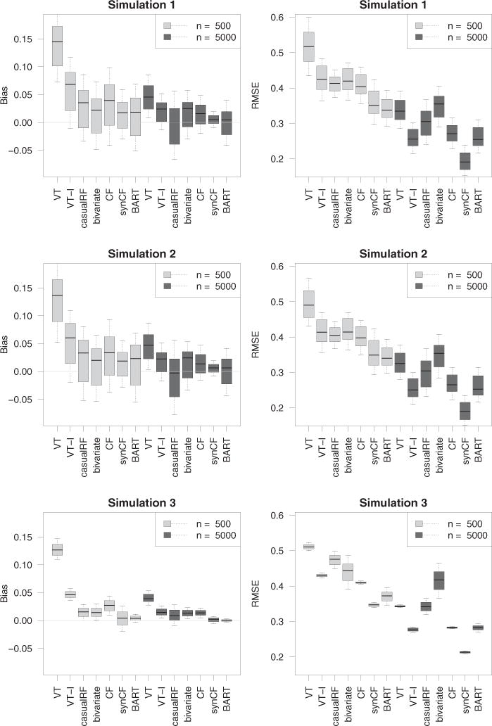
Bias and RMSE results from simulation experiments. Note that methods improve with increasing n.

Considering the RMSE results (right panels), it is clear that counterfactual synthetic forests, ${\widehat{\tau }}_{\text{synCF}}$, is generally the best of all procedures, with results improving with increasing n. The BART procedure, ${\widehat{\tau }}_{\text{BART}}$, is comparable or slightly better in simulations 1 and 2 when n = 500, but ${\widehat{\tau }}_{\text{synCF}}$ dominates when the sample size increases to n = 5000. In simulation 3, ${\widehat{\tau }}_{\text{synCF}}$ is superior regardless of sample size. It is interesting to observe that counterfactual forests, ${\widehat{\tau }}_{\text{CF}}$, which do not use synthetic forests for prediction, is systematically worse than ${\widehat{\tau }}_{\text{synCF}}$. In fact, its performance is generally about the same as ${\widehat{\tau }}_{\text{VT}-\mathrm{I}}$ and the same as ${\widehat{\tau }}_{\text{BART}}$ when n = 5000. Regarding ${\widehat{\tau }}_{\text{VT}-\mathrm{I}}$, it is interesting to observe how it systematically outperforms ${\widehat{\tau }}_{\text{VT}}$ regardless of simulation or sample size. This shows that augmenting the design matrix to include treatment interactions really improves adaptivity of VT forests. Finally, the least successful procedure (for the large sample size simulations) was the bivariate imputation method, ${\widehat{\tau }}_{\text{bivariate}}$. Recall that the bivariate procedure differs from the other procedures in that it uses mean imputation rather than regression modeling of the outcome for ITE estimation. This may explain its poorer performance. Following ${\widehat{\tau }}_{\text{bivariate}}$ in terms of overall performance, are ${\widehat{\tau }}_{\text{VT}}$ and ${\widehat{\tau }}_{\text{casualRF}}$, with ${\widehat{\tau }}_{\text{casualRF}}$ somewhere in between ${\widehat{\tau }}_{\text{VT}}$ and ${\widehat{\tau }}_{\text{VT}-\mathrm{I}}$. This completes the discussion of the RMSE. The results for bias (left panels) generally mirror those for RMSE. One interesting finding, however, is the tightness of the range of bias values for ${\widehat{\tau }}_{\text{synCF}}$ when n = 5000. This shows that with increasing sample size, ${\widehat{\tau }}_{\text{synCF}}$ gives consistently low bias even across extreme propensity score values.

3.4. The Impact of Heterogeneity

To assess effectiveness of methods to level of heterogeneity of treatment effect, we reran simulation 3 under a slight modification to f₃(X, T). We defined

$$\begin{gathered} f_3(\mathbf{X},T)=2.445-\gamma [1_{\{T=0\}}\times \sin (0.4X_1+0.154X_2 \\ -0.152X_{11}-0.126X_{12})-1_{\{T=1,h(\mathbf{X})<0\}}]. \end{gathered}$$

The value of γ was varied from small to large to induce low to high values of heterogeneity. We assessed level of heterogeneity by the statistic

$$h=\sqrt{\frac{\text{var}(\tau (\mathbf{X}))}{\text{var}(\epsilon )}}=\sqrt{\frac{\text{var}(\tau (\mathbf{X}))}{{\sigma }^2}}.$$

As illustration, the value γ = 1 used in the original simulation 3 yielded a heterogeneity of h = 6.5 (we note that using a similar modification to simulations 1 and 2 yielded values h = 6.4, 6.2). To assess the effect of heterogeneity, we reran simulation 3 with values γ = 0.5, 0.75, 1.5 corresponding to heterogeneities of h = 3.2, 4.8, 9.7. All experimental settings were kept the same. Simulations were run for the n = 500 sample size setting. The results are displayed in Figure S2 of the supplementary materials. As can be seen there, all methods improve with decreasing heterogeneity. Relative performance, however, remains the same.

4. Project Aware: A Counterfactual Approach to Understanding the Role of Drug Use in Sexual Risk

Project Aware was a randomized clinical trial performed in nine sexually transmitted disease clinics in the United States. The primary aim was to test whether brief risk-reduction counseling performed at the time of an HIV test had any impact on subsequent incidence of sexually transmitted infections (STIs). The results showed no impact of risk-reduction counseling on STIs. Neither were there any substance use interactions of the impact of risk-reduction counseling; however, substance use was associated with higher levels of STIs at follow-up. Other research has shown that substance use is associated with higher rates of HIV testing, and Black women showing the highest rates of HIV testing in substance use treatment clinics (Hernández et al. 2016). Since substance use is associated with risky sexual activity, detecting the dynamics of this relationship can contribute to preventive and educational efforts to control the spread of HIV. Our procedures for causal analysis of heterogeneity of effects in observational data should equalize the observed characteristics among substance use and nonsubstance use participants, thereby removing any impact of background imbalance in factors that may be related to relationship of substance use on sexual risk. Our procedure then allows an exploration of background factors that are truly related to this causal effect, conditional on all confounding factors being in the feature set.

To explore this issue of how substance use plays a role in sexual risk, we pursued an analysis in which the treatment (exposure) variable T was defined as drug use status of an individual (0 = no substance use in the prior 6 months, 1 = any substance use in the prior 6 months leading to the study). For the outcome, we used number of unprotected sex acts within the last 6 months as reported by the individual. Although Project Aware was randomized on the primary outcome (risk-reduction counseling), analysis of secondary outcomes such as substance use should be treated as if from an observational study. Indeed, unbalancedness of the data for drug use can be gleaned from Table 1, which displays results from a logistic regression in which drug use status was used for the dependent variable (n = 2813, p = 99). The list of significant variables suggests the data is unbalanced and indicates that inferential methods should be considered carefully. Thus, Table 2, which displays the results from a linear regression using number of unprotected sex acts as the dependent variable, should be interpreted with caution. Table 2 suggests there is no overall exposure effect of drug use, although several variables have significant drug interactions.

Table 1.

Illustration of unbalancedness of Aware data. Only significant variables (p-value < 0.05) from logistic regression analysis are displayed for clarity.

	Estimate	Std. error	Z	p-Value
Race	−028	0.11	−2.50	0.01
Chlamydia	0.34	0.15	2.30	0.02
Site 2	−0.62	0.16	−3.94	0.00
Site 4	−053	0.16	−3.23	0.00
Site 6	0.44	0.18	2.43	0.01
Site 7	−0.65	0.15	−4.22	0.00
Site 8	0.95	0.21	4.51	0.00
HIV risk	0.17	0.03	5.14	0.00
CESD	0.02	0.01	3.13	0.00
Condom change 2	−0.24	0.12	−2.07	0.04
Marriage	0.08	0.03	2.76	0.01
In Jail ever	0.42	0.10	4.07	0.00
AA/NA last 6 months 1	0.69	0.23	3.04	0.00
Frequency of injection	0.18	0.07	2.49	0.01
Gender	−0.39	0.10	−4.00	0.00

Table 2.

Naive causal effect analysis using linear regression where dependent variable is number of unprotected sex acts from Aware data. Only variables with p-value < 0.10 from regression analysis are displayed for clarity.

	Estimate	Std. error	Z	p-Value
Intercept	−5.06	22.17	−0.23	0.82
Drug	9.59	29.72	0.32	0.75
HCV2	8.14	4.09	1.99	0.05
Site 2	−14.00	6.82	−2.05	0.04
HIV risk	3.89	1.41	2.76	0.01
Condom change 3	−17.23	6.52	−2.64	0.01
Condom change 5	−21.98	6.65	−3.30	0.00
Visit ophthalmologist	−16.46	8.17	−2.01	0.04
Number visit ophthalmologist	9.13	3.93	2.33	0.02
Marriage	−2.13	1.17	−1.81	0.07
Smoke	53.13	16.26	3.27	0.00
Number cigarette per day	−14.63	4.76	−3.07	0.00
Drug × CESD	0.88	0.47	1.88	0.06
Drug × Condom change 2	−24.70	6.83	−3.62	0.00
Drug Condom × change 3	−25.82	8.75	−2.95	0.00
Drug Condom × change 4	−37.58	14.20	−2.65	0.01
Drug Condom × change 5	−28.78	9.33	−3.08	0.00
Drug Visit × dentist	−16.36	8.26	−1.98	0.05
Drug × Smoke	−34.71	20.53	−1.69	0.09
Drug × Number cigarette per day	9.81	5.95	1.65	0.10

To avoid drawing potentially flawed conclusions from an analysis like Table 2, we applied our counterfactual synthetic approach, ${\widehat{\tau }}_{\text{synCF}}$. Note that for this analysis to be correct, we rely on the assumption of SITA, which in this setting assumes drug use to be independent of number of unprotected sex acts with or without drug use, conditionally on X. With this caveat in mind, we applied our counterfactual approach by fitting a synthetic forest separately to each exposure group. Number of unprotected sex acts was used as the dependent variable. Estimated causal effects were defined as $\{{\widehat{\tau }}_{\text{synCF}}({\mathbf{x}}_i),i=1,\dots ,n\}$, where τ (x) equals mean difference in number of unprotected sex acts for drug versus nondrug users. These estimated causal effects were then used as dependent variables in a linear regression analysis. This was done because of the convenient interpretation of estimated coefficients in terms of subgroup causal differences (this point will be elaborated on shortly). To derive valid standard errors and confidence regions for the estimated coefficients, the entire procedure was subsampled. That is, we drew a sample of size m without replacement. The subsampled data were then fit using synthetic forests as described above, and the resulting estimated causal effects used as the dependent variable in a linear regression. The procedure was repeated 1000 times independently. A subsampling size of m = n/10 was used. The confidence regions of the resulting coefficients are displayed in Figure 2. Table 3 displays the coefficients for significant values (p-values < 0.05). We note that bootstrapping could have been used as another means to generate nonparametric p-values and confidence regions. However, we prefer subsampling because of its computational speed and general robustness (Politis, Romano, and Wolf 1999).

Figure 2.

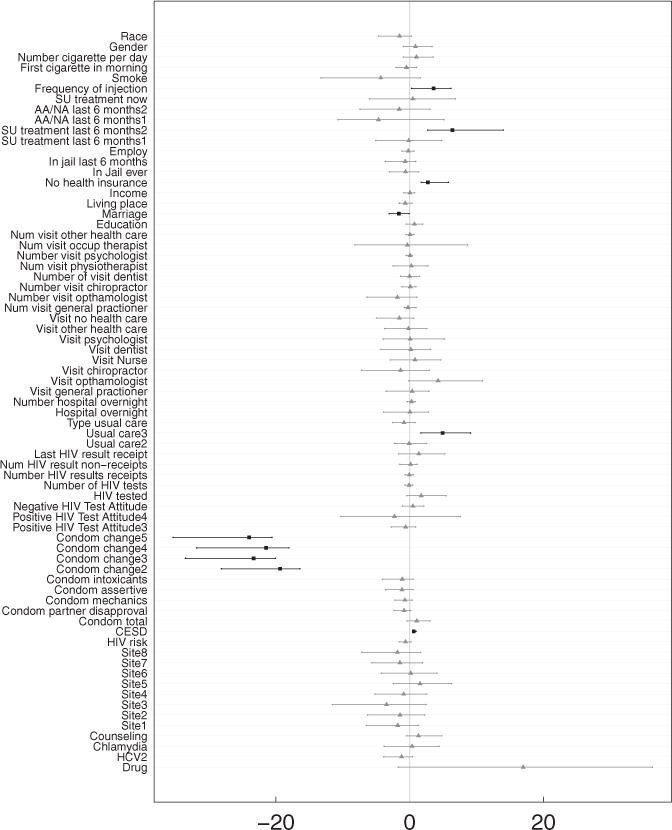
Assessing causal effects from counterfactual synthetic random forests analysis using linear regression (see Table 3). Displayed are confidence intervals for coefficients from linear model. Darker colored boxplots with squares indicate variables with p-value < 0.05.

Table 3.

Understanding causal effects from counterfactual synthetic random forests analysis using linear regression with dependent variable equal to the estimated causal effects $\{{\widehat{\tau }}_{\text{synCF}}({\mathbf{x}}_i),i=1,\dots ,n\}$. Causal effect is defined as the mean difference in unprotected sex acts for drug users versus nondrug users. Standard errors and significance of linear model coefficients were determined using subsampling. For clarity, only significant variables with p-value < 0.05 are displayed (the intercept is provided for reference but is not significant).

	Estimate	Std. error	Z
Intercept (drug use)	16.97	9.36	1.81
CESD	0.60	0.13	4.54
Condom change 2	−19.38	2.96	−6.56
Condom change 3	−23.33	3.23	−7.22
Condom change 4	−21.46	3.39	−6.32
Condom change 5	−24.02	3.41	−7.04
Usual care 3	4.91	2.11	2.33
Marriage	−1.61	0.73	−2.21
No health insurance	2.72	0.99	2.75
SU treatment last 6 months 2	6.38	3.20	2.00
Frequency of injection	3.59	1.77	2.02

To interpret the coefficients in Table 3, it is useful to write the true model for the outcome (number of unprotected sex acts) as Y = f (X, T) + ε, where

$$f(\mathbf{X},T)={\alpha }_{0}T+h(\mathbf{X},T),$$

and h is some unknown function. Under the assumption of SITA, and using the same calculations as (4), we have

$$\tau (\mathbf{x})=f(\mathbf{x},1)-f(\mathbf{x},0)={\alpha }_0+h(\mathbf{x},1)-h(\mathbf{x},0).$$

Now since we assume a linear model $\alpha +{\displaystyle {\sum }_{j=1}^p{\beta }_j{x}_j}$ for the ITE, we have

$${\alpha }_0+h(\mathbf{x},1)-h(\mathbf{x},0)=\alpha +{\displaystyle \sum _{j=1}^p{\beta }_j{x}_j}.$$

From this we can infer that the intercept in Table 3 is an overall measure of the exposure effect of drug use, α₀ (this is why the intercept term is listed as drug use). Here the estimated coefficient is 17.0. The positive coefficient implies that on average drug users have significantly more unprotected sex acts than nondrug users (significance here is slightly larger than 5%).

The remaining coefficients in Table 3 describe how the effect of drug use on sexual risk is modulated by other factors. Under our linear model, we have

$$h(\mathbf{x},1)-h(\mathbf{x},0)={\displaystyle \sum _{j=1}^p{\beta }_j{x}_j}.$$

Because h(x, 1) − h(x, 0) represents how much a subgroup deviates from the overall causal effect, each coefficient in Table 3 quantifies the effect of a specific subgroup on drug use differences. Consider, for example, the variable “Frequency of injection,” which is a continuous variable representing frequency of injections in drug users. Because its estimated coefficient is 3.6, this means the difference in unprotected sex acts between drug and nondrug users, which is positive, becomes even wider for high frequency drug users. Another risky factor is “No health insurance,” which is an indicator of lack of health insurance coverage. Because its estimated coefficient is 2.7, we can take this to mean that the increase in sexual risk for an individual without health insurance is more pronounced in drug users. As another example, consider the variable “Condom change,” which is an ordinal categorical variable measuring an individual’s stage of change with respect to condom use behavior. The baseline level is a “precontemplator,” who is an individual who has not envisioned using condoms. The second level “contemplator” is an individual contemplating using condoms. Further increasing levels measure even more willingness to use condoms. All coefficients for Condom change in Table 3 are negative, and therefore if an individual is more willing to use safe condom practice (relative to the baseline condition), the difference in number of unprotected sex acts diminishes between drug and nondrug users. Other variables that have a subgroup effect are Marriage (whether an individual is married), CESD (Center for Epidemiological Studies Depression Scale), and SU treatment last 6 months (substance abuse treatment in last 6 months). In all of these, the pattern is similar to before. With more risky behavior (with depression) the number of unprotected sex acts increases for nondrug users relative to drug users, but as risky behavior decreases (e.g., married), the effect of drug use diminishes.

Figure 3 displays a coplot of the RF estimated causal effects $\{{\widehat{\tau }}_{\text{synCF}}({\mathbf{x}}_i),i=1,\dots ,n\}$ as a function of several variables. The coplot is another useful tool that can be used to explore causal relationships. We use it to uncover relationships that may be hidden in the linear regression analysis. The RF causal effects are plotted against CESD depression for individuals with and without health insurance. Conditioning is on the variables Condom change (vertical conditioning) and HIV risk (horizontal conditioning). HIV risk a self-rated variable and of potential importance and was included even though it was not significant in the linear regression analysis. For patients with potential to change condom use (rows 2 through 5), increased depression levels leads to an increased causal effect of drug use, which is slightly accentuated for high HIV risk (plots going from left to right). The effect of health insurance is however minimal. On the other hand, for individuals with low potential to change condom use (bottom row), the estimated exposure effect is generally high, regardless of depression, but is reduced if the individual has health insurance.

Figure 3.

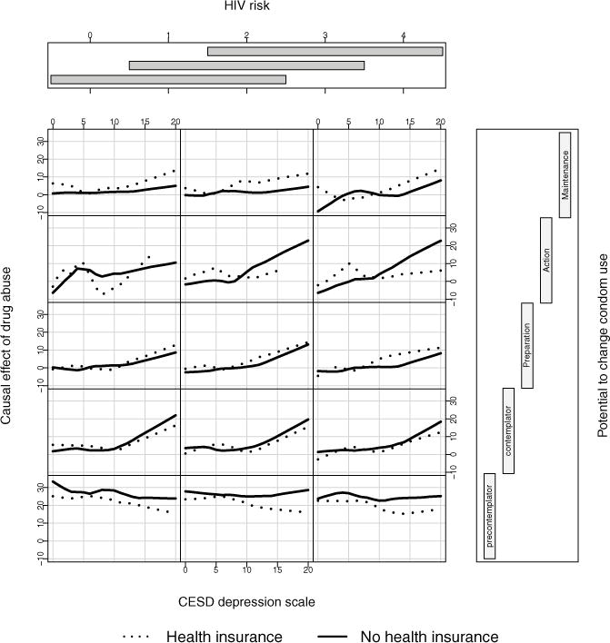
RF estimated causal effect of drug use plotted against CESD depression for individuals with and without health insurance. Values are conditioned on Condom change (vertical conditional axis) and HIV risk (horizontal conditional axis).

5. Discussion

In observational data with complex heterogeneity of treatment effect, individual estimates of treatment effect can be obtained in a principled way by directly modeling the response outcome. However, successful estimation mandates highly adaptive and accurate regression methodology and for this we relied on RF, a machine learning method with well-known properties for accurate estimation in complex nonparametric regression settings. However, care must be used when applying RF for casual inference. We encourage the use of out-of-bag estimation, a simple but underappreciated out-of-sample technique for improving accuracy. We also recommend that when selecting an RF approach, that it should have some means for encouraging adaptivity to confounding, that is, that it can accurately model potentially separate regression surfaces for each of the treatment groups. One example of this is the extension to VT, which expands the design matrix to include all pairwise interactions of variables with the treatment, a method we call ${\widehat{\tau }}_{\text{VT}-\mathrm{I}}$, and described in the article by Foster, Taylor, and Ruberg (2011). We found that this simple extension, when coupled with out-of-bagging, significantly improved performance of VT. Another promising method was counterfactual synthetic forests ${\widehat{\tau }}_{\text{synCF}}$, which generally had the best performance among all methods, and was superior in the larger sample size simulations, outperforming even the highly adaptive BART method. The larger sample size requirement is not so surprising as having to grow separate forests causes some loss of efficiency; this being however mitigated by its superior bias properties, which take hold with increasing n.

In looking back, we can now see that the success of counterfactual synthetic RF can be attributed to three separate effects: (a) fitting separate forests to each treatment group, which improves adaptivity to confounding; (b) replacing Breiman forests with synthetic forests, which reduces bias; and (c) using OOB estimation, which improves accuracy. Computationally, counterfactual synthetic RF are easily implemented with available software and have the added attraction that they reduce parameter tuning. The latter is a consequence and advantage of using synthetic forests. A synthetic forest is constructed using RF base learners, each of these being constructed under different nodesize and mtry tuning parameters. Correctly specifying mtry and nodesize is important for good performance in Breiman forests. The optimal value will depend on whether the setting is large n, large p, or large p and large n. With synthetic forests this problem is alleviated by building RF base learners under different tuning parameter values.

Importantly, and underlying all of this, is the potential outcomes model, a powerful hypothetical approach to causation. The challenge is being able to properly fit the potential outcomes model and for this, as discussed above, we relied on the sophisticated machinery of RF. We emphasize that the direct approach of the potential outcomes model is well suited for personalized inference via the ITE. Estimated ITE values from RF can be readily analyzed using standard regression models to yield direct inferential statements for not only overall treatment effect, but also interactions, thus facilitating inference beyond the traditional ATE population-centric viewpoint. Using the Aware data we showed how counterfactual ITE estimates from counterfactual synthetic forests could be explored to understand causal relations. This revealed interesting connections between risky behavior, drug use, and sexual risk. The analysis corrects for any observed differences by the exposure variable, so to the extent that we have observed the important confounding variables, this result can tentatively be considered causal, though caution should be used due to this assumption. Clearly, this type of analysis, which controls for observed confounding gives additional and important insights above simple observed drug usage differences. We also note that although we used linear regression for interpretation in this analysis, it is possible to use other methods as well. The counterfactual synthetic forest procedure provides a pipleline that can be connected with many types of analyses, such as the conditional plots that were also used in the Aware data analysis.

References

- Breiman L. Technical Report. University of California; Berkeley CA: 1996. Out-of-Bag Estimation. [Google Scholar]
- Breiman L. Random Forests. Machine Learning. 2001;45:5–32. [Google Scholar]
- Chipman H, McCulloch R. BayesTree: Bayesian Additive Regression Trees. R Package Version 0.3-1.4. 2016 Available at http://cran.r-project.org.
- Chipman HA, George EI, McCulloch RE. BART: Bayesian Additive Regression Trees. The Annals of Applied Statistics. 2010;4:266–298. [Google Scholar]
- Dasgupta A, Szymczak S, Moore JH, Bailey-Wilson JE, Malley JD. Risk Estimation Using Probability Machines. BioData Mining. 2014;7:1. doi: 10.1186/1756-0381-7-2. [DOI] [PMC free article] [PubMed] [Google Scholar]
- Foster JC, Taylor JM, Ruberg SJ. Subgroup Identification From Randomized Clinical Trial Data. Statistics in Medicine. 2011;30:2867–2880. doi: 10.1002/sim.4322. [DOI] [PMC free article] [PubMed] [Google Scholar]
- Ghosh D, Zhu Y, Coffman DL. Penalized Regression Procedures for Variable Selection in the Potential Outcomes Framework. Statistics in Medicine. 2015;34:1645–1658. doi: 10.1002/sim.6433. [DOI] [PMC free article] [PubMed] [Google Scholar]
- Hernández D, Feaster DJ, Gooden L, Douaihy A, Mandler R, Erickson SJ, Kyle T, Haynes L, Schwartz R, Das M, et al. Self-Reported HIV and HCV Screening Rates and Serostatus Among Substance Abuse Treatment Patients. AIDS and Behavior. 2016;20:204–214. doi: 10.1007/s10461-015-1074-2. [DOI] [PMC free article] [PubMed] [Google Scholar]
- Hill JL. Bayesian Nonparametric Modeling for Causal Inference. Journal of Computational and Graphical Statistics. 2011;20:217–240. [Google Scholar]
- Hirano K, Imbens GW, Ridder G. Efficient Estimation of Average Treatment Effects Using the Estimated Propensity Score. Econometrica. 2003;71:1161–1189. [Google Scholar]
- Ishwaran H, Kogalur U. Random Forests for Survival, Regression and Classification (RF-SRC) R Package Version 2.2.0. 2016 Available at http://cran.r-project.org.
- Ishwaran H, Kogalur UB, Blackstone EH, Lauer MS. Random Survival Forests. The Annals of Applied Statistics. 2008;2:841–860. [Google Scholar]
- Ishwaran H, Malley JD. Synthetic Learning Machines. BioData Mining. 2014;7:1. doi: 10.1186/s13040-014-0028-y. [DOI] [PMC free article] [PubMed] [Google Scholar]
- Lamont AE, Lyons M, Jaki TF, Stuart E, Feaster D, Ishwaran H, Tharmaratnam K, Van Horn ML. Identification of Predicted Individual Treatment Effects (PITE) in Randomized Clinical Trials. Statistical Methods in Medical Research. 2016 doi: 10.1177/0962280215623981. [DOI] [PubMed] [Google Scholar]
- Lee BK, Lessler J, Stuart EA. Improving Propensity Score Weighting Using Machine Learning. Statistics in Medicine. 2010;29:337–346. doi: 10.1002/sim.3782. [DOI] [PMC free article] [PubMed] [Google Scholar]
- Lunceford JK, Davidian M. Stratification and Weighting via the Propensity Score in Estimation of Causal Treatment Effects: A Comparative Study. Statistics in Medicine. 2004;23:2937–2960. doi: 10.1002/sim.1903. [DOI] [PubMed] [Google Scholar]
- Metsch LR, Feaster DJ, Gooden L, Schackman BR, Matheson T, Das M, Golden MR, Huffaker S, Haynes LF, Tross S, et al. Effect of Risk-Reduction Counseling With Rapid HIV Testing on Risk of Acquiring Sexually Transmitted Infections: The AWARE Randomized Clinical Trial. Journal of the American Medical Association. 2013;310:1701–1710. doi: 10.1001/jama.2013.280034. [DOI] [PMC free article] [PubMed] [Google Scholar]
- Neyman J, Dabrowska D, Speed T. On the Application of Probability Theory to Agricultural Experiments. Essay on Principles. Section 9. Statistical Science. 1990;5:465–472. [Google Scholar]
- Politis DN, Romano JP, Wolf M. Subsampling Springer Series in Statistics. Berlin: Springer; 1999. [Google Scholar]
- Robins JM, Greenland S, Hu FC. Estimation of the Causal Effect of a Time-Varying Exposure on the Marginal Mean of a Repeated Binary Outcome. Journal of the American Statistical Association. 1999;94:687–700. [Google Scholar]
- Rosenbaum PR, Rubin DB. The Central Role of the Propensity Score in Observational Studies for Causal Effects. Biometrika. 1983;70:41–55. [Google Scholar]
- Rubin DB. Estimating Causal Effects of Treatments in Randomized and Nonrandomized Studies. Journal of Educational Psychology. 1974;66:688. [Google Scholar]
- Rubin DB. The Design Versus the Analysis of Observational Studies for Causal Effects: Parallels With the Design of Randomized Trials. Statistics in Medicine. 2007;26:20–36. doi: 10.1002/sim.2739. [DOI] [PubMed] [Google Scholar]
- Su X, Meneses K, McNees P, Johnson WO. Interaction Trees: Exploring the Differential Effects of an Intervention Programme for Breast Cancer Survivors. Journal of the Royal Statistical Society, Series C. 2011;60:457–474. [Google Scholar]
- Su X, Tsai CL, Wang H, Nickerson DM, Li B. Subgroup Analysis via Recursive Partitioning. The Journal of Machine Learning Research. 2009;10:141–158. [Google Scholar]
- Tang F, Ishwaran H. Random Forest Missing Data Algorithms. Statistical Analysis and Data Mining. 2017 doi: 10.1002/sam.11348. [DOI] [PMC free article] [PubMed] [Google Scholar]
- Tricoci P, Allen JM, Kramer JM, Califf RM, Smith SC. Scientific Evidence Underlying the ACC/AHA Clinical Practice Guidelines. Journal of the American Medical Association. 2009;301:831–841. doi: 10.1001/jama.2009.205. [DOI] [PubMed] [Google Scholar]
- Wager S, Athey S. Journal of the American Statistical Association. 2017. Estimation and Inference of Heterogeneous Treatment Effects Using Random Forests. [Google Scholar]
Associated Data
This section collects any data citations, data availability statements, or supplementary materials included in this article.