Dice Overlap Measures for Objects of Unknown Number: Application to Lesion Segmentation

Abstract

The Dice overlap ratio is commonly used to evaluate the performance of image segmentation algorithms. While Dice overlap is very useful as a standardized quantitative measure of segmentation accuracy in many applications, it offers a very limited picture of segmentation quality in complex segmentation tasks where the number of target objects is not known a priori, such as the segmentation of white matter lesions or lung nodules. While Dice overlap can still be used in these applications, segmentation algorithms may perform quite differently in ways not reflected by differences in their Dice score. Here we propose a new set of evaluation techniques that offer new insights into the behavior of segmentation algorithms. We illustrate these techniques with a case study comparing two popular multiple sclerosis (MS) lesion segmentation algorithms: OASIS and LesionTOADS.

1 Introduction

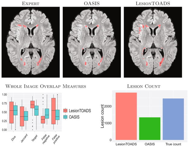
Segmentation is a broad and critical field of research in medical image analysis. The evaluation of segmentation algorithms is crucial both for assessing the performance of new algorithms and for choosing a particular algorithm for a new task. In medical image segmentation, the Dice [6] and Jaccard [11] overlap ratios are the most popular evaluation measures [16,22]. The mean and maximum surface distances between 3D objects are also commonly used to evaluate segmentation algorithms [9], as are distances between segmentation results and manual landmarks. However, such measures are based on the implicit assumption that the number of segmentation targets is known a priori, e.g., whether it is one liver, two hippocampi, or five lung lobes. This is in contrast to a different but equally important class of segmentation tasks, such as the segmentation of white matter lesions or lung nodules, where the number of target objects can vary from zero to hundreds or more. In these scenarios, the object detection and segmentation tasks become intertwined and as such, performance evaluation needs to take both aspects into consideration. Although, it has been customary to use the image-wide Dice overlap in these combined detection and segmentation problems, this is an oversimplification and can often hide differences in algorithm behaviors (e.g., Fig. 1). Another popular criterion in these types of applications is the number of segmented objects, which attempts to evaluate the detection success. However, the object count alone is an ambiguous metric as it reflects not only the false positive and false negative detections but also larger objects that may be erroneously split into multiple smaller ones, or multiple small objects erroneously merged into a single, larger object. Furthermore, these commonly used metrics fail to relate the size of the object to the final score, which can be important: for many applications, an algorithm that misses large objects is considered less clinically relevant than an algorithm that misses small objects.

Fig. 1.

The top row shows a typical example of segmentation results for the two algorithms and expert delineation. The second row shows image-wide overlap measures and the lesion count for both methods and the expert delineation (True count).

A prime example of an application domain with a variable number of objects is multiple sclerosis (MS) lesion segmentation from MRI scans of the brain. White matter lesions are the hallmark of MS and their segmentation and quantification are critical for clinical purposes. Many approaches to MS lesion segmentation have been proposed: artificial [10] and convolutional neural networks [1]; Bayesian models [7]; Gaussian mixture models [23]; graph cuts [8]; and random forests [12]. This field of research remains very active and several grand challenges (MICCAI 2008 [19], ISBI 2015 [2], MICCAI 2016 [13]) have been organized in recent years. The evaluation of new algorithms often relies on Dice and Jaccard overlaps and lesion counts, which limits our ability to fully assess other characteristics in performance difference.

We propose a new set of evaluation techniques to compare segmentations with a variable number of target objects, including a classification of segmentation results and statistics at object and category levels. We illustrate these techniques in an MS lesion segmentation study comparing two algorithms: LesionTOADS [17] which is an unsupervised clustering algorithm with topological constraints; and OASIS [21] is a supervised classifier based on multi-modal logistic regression.

2 Methods

2.1 Data and Compared Methods

As a case study, we used a set of T1w, T2w, PD, and FLAIR images from 70 MS patients acquired at 3T. The images of each subject were co-registered rigidly to the T1w space, which was also rigidly aligned to the MNI template. Lesions were manually segmented in each T1w-FLAIR pair by an expert with more than 15 years of experience. Two popular algorithms, OASIS [21] and LesionTOADS [17], were applied to this dataset. For OASIS, data from a disjoint set of 20 MS patients imaged with the same protocol were used for training. LesionTOADS was run with T1w and FLAIR inputs; the smoothing parameter was adjusted from 0.2 to 0.4 as we empirically found this to improve the quality of the segmentations and a different weight (0.7 vs. 1.0 vs. 1.2) was used for the FLAIR image in the multi-channel segmentation based on the lesion load (Low vs. Med. vs. High)—see Shiee et al. [18] for details.

2.2 Object Correspondence Identification and Classification

Given a pair of segmentations S_i1 and S_i2 ∈ {0, 1}^V for a subject i, e.g., an automated and a manual segmentation, respectively, we begin by identifying the (6-) connected components in each segmentation as individual objects (i.e., lesions in our application). We name these two sets of objects C_i1 and C_i2. Then, for each object in C_i1, we identify its corresponding objects by determining all objects in C_i2 (if any) that it overlaps with. Formally, for an object O_ij1 ∈ C_i1, the set of matching objects is m(O_ij1) = {O_ik2, ∀k : O_ij1 ∩ O_ik2 ≠ ∅}. Note that this means 0, 1, or multiple corresponding objects are possible. Similarly, for each object O_ij2 ∈ C_i2, we identify its set of corresponding objects, m(O_ij2), by determining all objects in C_i1 (if any) that it overlaps with.

Following correspondence identification, it is possible to determine the match configuration for each object by considering the number of forward and backward correspondences. For example, if an object O_ij1 ∈ C_i1 corresponds to a single object O_ik2 ∈ C_i2, and O_ik2 corresponds to a single object (i.e., O_ij1), then we have a 1-1 match. In contrast, if an object O_ij1 ∈ C_i1 corresponds to multiple objects O_i12-O_iN2, and each of the O_i·2 correspond only to O_ij1, then we have a 1-N match. Following the nomenclature of [15], we have the following categories:

• Correct detection: 1-1 match.

• False alarm: 1-0 match. An object exists in C_i1 that does not exist in C_i2, i.e., a false positive if C_i2 is the truth.

• Merge: 1-N match. Multiple objects in C_i2 are merged into a single object in C_i1.

• Split: N-1 match. A single object in C_i2 is split into multiple objects in C_i1.

• Split-merge: N-N match. The conditions for both merge and split are satisfied.

• Detection failure: 0–1 match. An object exists in C_i2 that does not exist in C_i1, i.e., a false negative if C_i2 is the truth.

We note that while the results presented in this paper focus on the comparison of an automated segmentation S_i1 and a manual segmentation S_i2, the same idea for classification can also be applied to the comparison of two manual segmentations to assess intra- or inter-rater variability, as well as to segmentations from different timepoints in a longitudinal study to assess the disease course.

2.3 Lesion Segmentation Evaluation

We propose a battery of statistics to compare two binary segmentations for a subject i, S_i1 and S_i2, which will be illustrated in Sect. 3.

We begin by reporting the classical image-wide overlap measures. In particular, for each subject i, we report the Dice overlap ( ${\text{DSC}}_i=2\frac{\mid S_{i1}\cap S_{i2}\mid }{\mid S_{i1}\mid +\mid S_{i2}\mid }$) [6], the Jaccard overlap ( $2\frac{\mid S_{i1}\cap S_{i2}\mid }{\mid S_{i1}\cup S_{i2}\mid }$) [11], target overlap ( $\frac{\mid S_{i1}\cap S_{i2}\mid }{S_{i2}}$), the false negative error ( $\frac{\mid S_{i2}-S_{i1}\mid }{\mid S_{i2}\mid }$) and the false positive error ( $\frac{\mid S_{i1}-S_{i2}\mid }{\mid S_{i1}\mid }$). We also report the number of connected objects (|C_i1|), which is another popular evaluation measure.

Next, we classify the object segmentation as described in Sect. 2.2 and report the number of objects n_ik1 and n_ik2, defined by S_i1 and S_i2, in each category k. We further report the average per-object Dice overlap, $\overline{{\text{DSC}}_{ik1}}=n_{ik1}^{-1}{\sum }_{j=1}^{n_{ik1}}{\text{DSC}}_{\mathit{ijk}}$, for each category k, where DSC_ijk is the Dice of an object j, defined as the Dice overlap between the segmentation of the j^th object of type k in S_i1, O_ijk1, and the matching set m(O_ijk1).

Next, we analyze the mean per-object Dice overlap as a function of true object size, i.e., f(s) = 𝔼(DSC_ijk | |O_ijk| = s), where |·| denotes the volume of an object and 𝔼 is the expectation operator. This is done both globally for all objects, as well as separately for each category of matches (which we denote by f_k(s)), using locally weighted scatterplot smoothing (LOESS) [3]. We use scatterplots of Dice vs. true object size to visualize this data. To estimate 95% confidence bands for the LOESS scatterplots, we use a nonparametric bootstrap. We resample by subject to respect the nested object-within-subject correlation structure. That is, for each b ∈ [1, 10000], we resample subjects i ∈ [1, n] with replacement to form a bootstrapped sample of pairs of segmentations $(S_{11}^{(b)},S_{12}^{(b)}),\dots ,(S_{n1}^{(b)},S_{n2}^{(b)})$ and re-estimate f(s), and f_k(s) and denote these estimates by f̂^(b)(s), and ${\widehat{f}}_k^{(b)}(s)$. We then calculate the pointwise 2.5% and 97.5% quantiles of f̂^(b) and ${\widehat{f}}_k^{(b)}$ to estimate the lower and upper limits of confidence bands. For the false alarm and correct detection classes, we use histograms of object size (since the Dice is always 0 for these classes). Additionally, for these two classes, we report the spatial distribution of the occurrences by registering all images into a common atlas space to construct a spatial occurrence frequency map.

3 Results

Figure 1 shows a summary of the whole-image overlap measures. LesionTOADS and OASIS have comparable Dice and Jaccard measures, which is important since these are two of the most commonly used measures for comparing segmentation algorithms. LesionTOADS has a smaller false negative ratio but a higher false positive ratio than OASIS. The number of distinct lesions as segmented by the expert manual rater was 2461; OASIS detected 1340 distinct lesions whereas LesionTOADS detected 2810. LesionTOADS reports more lesions than OASIS, but it is uncertain using these measures whether this is driven by a higher successful detection rate, more false alarms, more split lesions, or other reasons.

Figure 2(a) shows the per-lesion Dice overlap, summarized per class. Note that the Dice for the detection failures and false alarms is 0 by construction. The LesionTOADS algorithm has a higher Dice than OASIS in every category, which is rather surprising given that the whole-image Dice measures are nearly equal between the two methods (see Fig. 1). Figure 2(b) shows the number of lesions in each of the classes described in Sect. 2. Compared to overall lesion counts, this analysis provides further insight into the algorithm behavior: compared to OASIS, LesionTOADS has a larger number of correctly detected lesions (good), and fewer detection failures (good), but also more merges (bad), and many more false alarms (bad). As such, it is difficult to declare an overall “winner” but each algorithm is “winning” for different classes of lesions.

Fig. 2.

For both LesionTOADS and OASIS, we show the (a) Dice overlap by lesion class and the (b) lesion count by class.

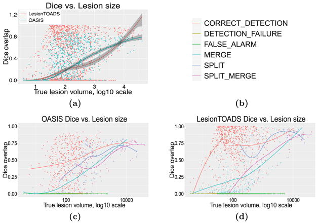
Figure 3(a) shows the per-lesion Dice overlap as a function of true lesion size. On average, LesionTOADS seems to perform better than OASIS for small and large lesions, whereas OASIS performs better for the more prevalent mediumsized lesions. It is also interesting that in this medium-size range, OASIS appears to have a tighter distribution of Dice scores whereas LesionTOADS performs either very well (Dice > 0.8) or very poorly (Dice < 0.2). Figures 3(c) and (d) provide additional insight by breaking down this data into individual classes.

Fig. 3.

(a) For both LesionTOADS and OASIS, we show per-lesion Dice overlap as a function of true lesion size, bootstrapped per subject. Per-lesion Dice overlap as a function of true lesion size, color-coded by classification (see legend in (b)), for both (c) OASIS and (d) LesionTOADS.

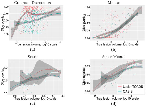
Figure 4 takes this analysis one step further by directly comparing the algorithms’ behaviors in each class. Figure 4(a) shows this comparison for the correctly detected lesions. We note that the average performance of the LesionTOADS algorithm increases steeply with size in this class, indicating the algorithm is highly accurate for all but the smallest lesions (which are notoriously difficult to segment correctly), for those lesions that it manages to detect correctly. In contrast, OASIS performance improves more slowly with lesion size. Figure 4(b) compares the two methods for merged lesions; while the performance of the two algorithms are roughly comparable and both improve with lesion size, there are overall fewer merged lesions for OASIS, which is desirable. Figures 4(c) and (d) provide the same comparison for split and split-merge classes, respectively.

Fig. 4.

Per-lesion Dice overlap vs. true lesion size, bootstrapped per subject.

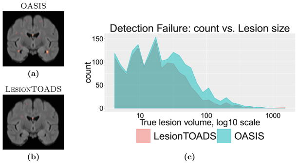
For false alarms and detection failures, instead of scatterplots, we present spatial distribution maps and size histograms of lesions. Figure 5 shows the detection failures for the two algorithms. It is interesting that the distribution of these failures are remarkably similar between the two algorithms for smaller lesions, suggesting many of these smaller lesions may be generally difficult to detect. The spatial distributions of these detection failures concentrate on the septum area for both methods. OASIS has an additional hotspot for detection failures near the temporal horn of the ventricles.

Fig. 5.

Spatial distribution of detection failures on a coronal slice for (a) OASIS and (b) LesionTOADS, with both methods exhibiting failures around the septum. Size statistics of detection failures for (c) both OASIS and LesionTOADS.

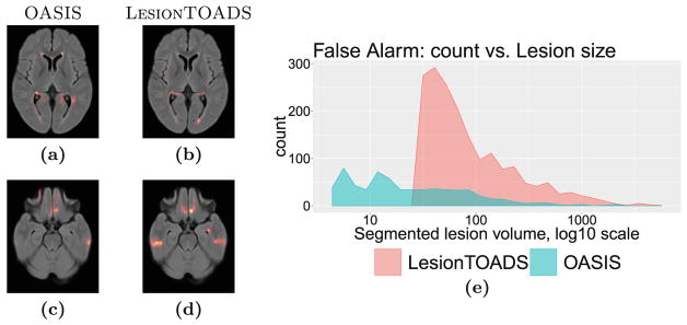
Figure 6 compares the false alarms for the two algorithms. LesionTOADS appears to generate hardly any small false positive lesions, but many medium-to-large false positive lesions. This rather surprising finding explains the counterintuitive result that while LesionTOADS reports better Dice overlap for each lesion category (Fig. 2), the whole-image Dice scores are nearly identical between the two methods (see Fig. 1). We note that the large number of false alarms reported for LesionTOADS is likely due to the use of a limited range of parameters for this study for a fair comparison to OASIS. In other use scenarios, LesionTOADS could be run with different parameter settings for each patient. Furthermore, it is striking that two algorithms with such similar whole-image Dice scores can have such dramatically different performance in different types of lesions, which can go unnoticed in studies that only report the whole-image Dice score. The spatial distributions of false alarms concentrate around the ventricles as well as the inferior brain for both methods; the latter region is especially pronounced for LesionTOADS.

Fig. 6.

False alarm category. Spatial distribution for (a, c) OASIS and (b, d) LesionTOADS, and (e) size statistics. LesionTOADS appears to generate hardly any small false positive lesions, but many medium-to-large false positive lesions.

4 Discussion

We have presented a battery of new complementary measures to better evaluate the performance of segmentation algorithms. Detailed evaluations can also be useful for parameter tuning: algorithms typically require multiple parameters to be set and the effects of changing these parameters are not always clear based on image-wide Dice alone. While the current study focuses on the MS lesion segmentation task, the presented evaluation scheme is directly applicable to other segmentation tasks where the object of interest is of variable number, such as lung nodule segmentation and cell counting. Additionally, even when the number of objects is known a priori, it has been argued [4] that reducing the segmentation quality to a single value represented by the Dice or Haussdorff score may be an oversimplification, and that a more detailed evaluation scheme may be beneficial.

The results in our case study highlight a common problem with the popular evaluation approach that relies only on Dice overlap: two algorithms with have nearly identical overall Dice overlap ratios, but digging deeper reveals that the behaviors of the algorithms are dramatically different. Additionally, in this particular study, the number of false alarms happens to be consistent with the image-wide false negative rate, and the number of detection failures happens to be consistent with the image-wide false positive rate. However, this does not have to be the case, as multiple small missed lesions and few large missed lesions are indistinguishable in the image-wide measures; similarly for multiple small false positive lesions and few large false positive lesions.

It is well known that the pathology of large lesions may often be different than that of smaller lesions; multiple small lesions are not equivalent to a single large lesion in terms of white matter damage, even if their overall size and location may be similar. Therefore, in addition to their relevance for shedding light onto the overall performance of segmentation algorithms, the Split, Merge, and Split-Merge categories are also potentially clinically relevant. Moreover, in longitudinal studies, it is often desired to “track” lesions over time [14,20], and thus analysis of the merging behavior can also be highly relevant in such studies.

One potential weakness of the present study is that the identification of overlapping lesions is currently performed with no tolerance; i.e., if two lesions overlap by even a single voxel, they are considered to be in correspondence. While it would be straightforward to modify this to allow a threshold of tolerance (e.g., only consider it a match if X voxels or Y % of the true lesion volume are overlapping), this would add a layer of complexity to the interpretation of the results. The connectivity could also be extended beyond just 6-connectivity. These concerns can be taken into account similar to the multi-label evaluation approach in [5] that considers fuzzy segmentations. Further, while it would be straightforward to also report Jaccard, target overlap, false negative, and false positive errors at the per-lesion scale, here we focused on Dice for the sake of brevity. However, such metrics would likely provide additional insights into algorithm behavior. These additional analyses will be performed in future work.

References

- 1.Birenbaum A, Greenspan H. Multi-view longitudinal CNN for multiple sclerosis lesion segmentation. Eng Appl Artif Intell. 2017;65:111–118. [Google Scholar]
- 2.Carass A, Roy S, Jog A, Cuzzocreo JL, Magrath E, Gherman A, Button J, Nguyen J, Prados F, Sudre CH, Cardoso MJ, Cawley N, Ciccarelli O, Wheeler-Kingshott CAM, Ourselin S, Catanese L, Deshpande H, Maurel P, Commowick O, Barillot C, Tomas-Fernandez X, Warfield SK, Vaidya S, Chunduru A, Muthuganapathy R, Krishnamurthi G, Jesson A, Arbel T, Maier O, Handels H, Iheme LO, Unay D, Jain S, Sima DM, Smeets D, Ghafoorian M, Platel B, Birenbaum A, Greenspan H, Bazin PL, Calabresi PA, Crainiceanu C, Ellingsen LM, Reich DS, Prince JL, Pham DL. Longitudinal multiple sclerosis lesion segmentation: resource & challenge. NeuroImage. 2017;148:77–102. doi: 10.1016/j.neuroimage.2016.12.064. [DOI] [PMC free article] [PubMed] [Google Scholar]
- 3.Cleveland WS. Robust locally weighted regression and smoothing scatterplots. J Am Stat Assoc. 1979;74(368):829–836. [Google Scholar]
- 4.Crimi A. Brain lesions, introduction. In: Crimi A, Menze B, Maier O, Reyes M, Handels H, editors. BrainLes 2015. LNCS. Vol. 9556. Springer; Cham: 2016. pp. 1–5. [DOI] [Google Scholar]
- 5.Crum WR, Camara O, Hill DLG. Generalized overlap measures for evaluation and validation in medical image analysis. IEEE Trans Med Imag. 2006;25(11):1451–1461. doi: 10.1109/TMI.2006.880587. [DOI] [PubMed] [Google Scholar]
- 6.Dice LR. Measures of the amount of ecologic association between species. Ecology. 1945;26(3):297–302. [Google Scholar]
- 7.Elliott C, Arnold DL, Collins DL, Arbel T. Temporally consistent probabilistic detection of new multiple sclerosis lesions in brain MRI. IEEE Trans Med Imag. 2013;32(8):1490–1503. doi: 10.1109/TMI.2013.2258403. [DOI] [PubMed] [Google Scholar]
- 8.García-Lorenzo D, Lecoeur J, Arnold DL, Collins DL, Barillot C. Multiple sclerosis lesion segmentation using an automatic multimodal graph cuts. In: Yang G-Z, Hawkes D, Rueckert D, Noble A, Taylor C, editors. MICCAI 2009. LNCS. Vol. 5762. Springer; Heidelberg: 2009. pp. 584–591. [DOI] [PubMed] [Google Scholar]
- 9.Gerig G, Jomier M, Chakos M. Valmet: a new validation tool for assessing and improving 3D object segmentation. In: Niessen WJ, Viergever MA, editors. MICCAI 2001. LNCS. Vol. 2208. Springer; Heidelberg: 2001. pp. 516–523. [DOI] [Google Scholar]
- 10.Goldberg-Zimring D, Achiron A, Miron S, Faibel M, Azhari H. Automated detection and characterization of multiple sclerosis lesions in brain MR images. Mag Reson Imaging. 1998;16(3):311–318. doi: 10.1016/s0730-725x(97)00300-7. [DOI] [PubMed] [Google Scholar]
- 11.Jaccard P. The distribution of the flora in the alpine zone. New Phytol. 1912;11(2):37–50. [Google Scholar]
- 12.Jog A, Carass A, Pham DL, Prince JL. Multi-output decision trees for lesion segmentation in multiple sclerosis. Proceedings of SPIE Medical Imaging (SPIE-MI 2015); Orlando, FL. 21–26 February 2015; 2015. pp. 94131C–94131C-6. [DOI] [PMC free article] [PubMed] [Google Scholar]
- 13.Maier O, Menze BH, von der Gablentz J, Häni L, Heinrich MP, Liebrand M, Winzeck S, Basit A, Bentley P, Chen L, Christiaens D, Dutil F, Egger K, Feng C, Glocker B, Götz M, Haeck T, Halme HL, Havaei M, Iftekharuddin KM, Jodoin PM, Kamnitsas K, Kellner E, Korvenoja A, Larochelle H, Ledig C, Lee JH, Maes F, Mahmood Q, Maier-Hein KH, McKinley R, Muschelli J, Pal C, Pei L, Rangarajan JR, Reza SMS, Robben D, Rueckert D, Salli E, Suetens P, Wang CW, Wilms M, Kirschke JS, Krämer UM, Münte TF, Schramm P, Wiest R, Handels H, Reyes M. ISLES 2015 - a public evaluation benchmark for ischemic stroke lesion segmentation from multispectral MRI. Med Image Anal. 2017;35:250–269. doi: 10.1016/j.media.2016.07.009. [DOI] [PMC free article] [PubMed] [Google Scholar]
- 14.Meier DS, Guttmann CRG. MRI time series modeling of MS lesion development. NeuroImage. 2006;32(2):531–537. doi: 10.1016/j.neuroimage.2006.04.181. [DOI] [PubMed] [Google Scholar]
- 15.Nascimento JC, Marques JS. Performance evaluation of object detection algorithms for video surveillance. IEEE Trans Multimed. 2006;8(4):761–774. [Google Scholar]
- 16.Rohlfing T. Image similarity and tissue overlaps as surrogates for image registration accuracy: widely used but unreliable. IEEE Trans Med Imaging. 2012;31(2):153–163. doi: 10.1109/TMI.2011.2163944. [DOI] [PMC free article] [PubMed] [Google Scholar]
- 17.Shiee N, Bazin PL, Ozturk A, Reich DS, Calabresi PA, Pham DL. A topology-preserving approach to the segmentation of brain images with multiple sclerosis lesions. NeuroImage. 2010;49(2):1524–1535. doi: 10.1016/j.neuroimage.2009.09.005. [DOI] [PMC free article] [PubMed] [Google Scholar]
- 18.Shiee N, Bazin PL, Zackowski K, Farrell SK, Harrison DM, Newsome SD, Ratchford JN, Caffo BS, Calabresi PA, Pham DL, Reich DS. Revisiting brain atrophy and its relationship to disability in multiple sclerosis. PLoS ONE. 2012;7(5):e37049. doi: 10.1371/journal.pone.0037049. [DOI] [PMC free article] [PubMed] [Google Scholar]
- 19.Styner M, Lee J, Chin B, Chin MS, Commowick O, Tran HH, Markovic-Plese S, Jewells V, Warfield S. 3D segmentation in the clinic: a grand challenge II: MS lesion segmentation. 11th International Conference on Medical Image Computing and Computer Assisted Intervention (MICCAI 2008) 3D Segmentation in the Clinic: A Grand Challenge II; 2008. pp. 1–6. [Google Scholar]
- 20.Sweeney EM, Shinohara RT, Dewey BE, Schindler MK, Muschelli J, Reich DS, Crainiceanu CM, Eloyan A. Relating multi-sequence longitudinal intensity profiles and clinical covariates in incident multiple sclerosis lesions. NeuroImage Clin. 2016;10:1–17. doi: 10.1016/j.nicl.2015.10.013. [DOI] [PMC free article] [PubMed] [Google Scholar]
- 21.Sweeney EM, Shinohara RT, Shiee N, Mateen FJ, Chudgar AA, Cuzzocreo JL, Calabresi PA, Pham DL, Reich DS, Crainiceanu CM. OASIS is automated statistical inference for segmentation, with applications to multiple sclerosis lesion segmentation in MRI. NeuroImage Clin. 2013;2:402–413. doi: 10.1016/j.nicl.2013.03.002. [DOI] [PMC free article] [PubMed] [Google Scholar]
- 22.Taha AA, Hanbury A. Metrics for evaluating 3D medical image segmentation: analysis, selection, and tool. BMC Med Imaging. 2015;15(1):29. doi: 10.1186/s12880-015-0068-x. [DOI] [PMC free article] [PubMed] [Google Scholar]
- 23.Tomas-Fernandez X, Warfield SK. A model of population and subject (MOPS) intensities with application to multiple sclerosis lesion segmentation. IEEE Trans Med Imaging. 2015;34(6):1349–1361. doi: 10.1109/TMI.2015.2393853. [DOI] [PMC free article] [PubMed] [Google Scholar]