Cox Regression Model with Doubly Truncated Data

Abstract

Truncation is a well-known phenomenon that may be present in observational studies of time-to-event data. While many methods exist to adjust for either left or right truncation, there are very few methods that adjust for simultaneous left and right truncation, also known as double truncation. We propose a Cox regression model to adjust for this double truncation using a weighted estimating equation approach, where the weights are estimated from the data both parametrically and nonparametrically, and are inversely proportional to the probability that a subject is observed. The resulting weighted estimators of the hazard ratio are consistent. The parametric weighted estimator is asymptotically normal and a consistent estimator of the asymptotic variance is provided. For the nonparametric weighted estimator, we apply the bootstrap technique to estimate the variance and confidence intervals. We demonstrate through extensive simulations that the proposed estimators greatly reduce the bias compared to the unweighted Cox regression estimator which ignores truncation. We illustrate our approach in an analysis of autopsy-confirmed Alzheimer’s disease patients to assess the effect of education on survival.

1. Introduction

Accurate regression coefficient estimation in survival analysis is crucial for studying factors that affect disease progression. However in some survival studies the outcome of interest may be subject to either left or right truncation. When both left and right truncation are present, this is known as double truncation. For example, double truncation is inherent in retrospective autopsy-confirmed studies of Alzheimer’s disease (AD), where autopsy confirmation is the gold standard for diagnosing AD due to the inaccuracy of clinical diagnosis (Beach et al. 2012). The right truncation occurs because information is only obtained from a subject when they receive an autopsy. Subjects who survive past the end of the study are not diagnosed and therefore not included in the study sample, resulting in a sample that is biased towards subjects with smaller survival times. Furthermore, the retrospective sample is also left truncated because subjects who succumb to the disease before they enter the study are unobserved, resulting in a sample that is biased towards subjects with larger survival times. A diagram showing how double truncation occurs is provided in Figure 1. We note that right censoring is not possible in this setting, since any subject who has an autopsy performed will also have a known survival time.

Figure 1.

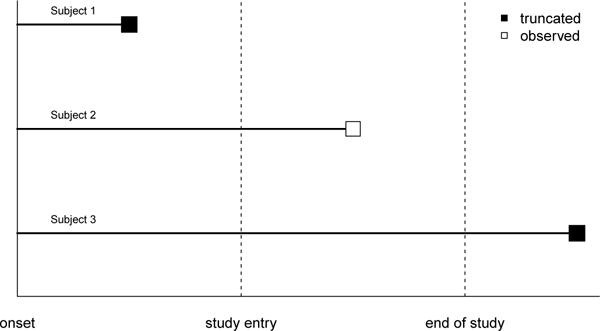
In this hypothetical example, we assume subjects 1, 2, and 3 all have similar times of disease symptom onset. For illustrative purposes, we also assume that subjects 1, 2, and 3 have the same study entry time, however this need not be the case. Here the x-axis represents time, and the squares represent the terminating events. Subject 1 is left truncated because they die before they enter the study. Subject 2 enters the study and dies before the end of the study, and is therefore observed. Subject 3 is right truncated because they live past the end of the study, and therefore do not have an autopsy performed.

If the left and right truncation are not accounted for then the observed sample will be biased, which may lead to biased estimators of regression coefficients and hazard ratios. In this paper, we examine the relationship between education and survival from AD symptom onset in a retrospective autopsy-confirmed AD population. The default application for analysis in this setting is the Cox regression model (Cox 1972). However, to obtain consistent regression coefficient estimators, we must adjust for truncation. Regression techniques already exist under left truncation (Lai and Ying 1991), right truncation (Kalbfleisch and Lawless 1991), and length-biased data (Wang 1996). In this paper, we propose a Cox regression model to adjust for double truncation using a weighted estimating equation approach, where the hazard rate for the failure times follows that of the standard Cox regression model.

Although double truncation may appear in many studies in which data is only recorded for subjects whose event times fall in an observable time interval, the amount of literature on methods to handle double truncation is small. Most of the literature deals with the estimation of the survival distribution rather than regression. Efron and Petrosian (1999) introduced the nonparametric maximum likelihood estimator (NPMLE) for the survival distribution function under double truncation. Shen (2010a) investigated the asymptotic properties of the NPMLE and introduced a nonparametric estimator of the truncation distribution function. Shen (2010b) and Moreira and de Ũna-Álvarez (2010) introduced a semiparametric maximum likelihood estimator (SPMLE) for the survival distribution function under double truncation. Shen (2013) introduced a method for regression analysis of interval censored and doubly truncated data using linear transformation models, but these models only allow discrete covariates and the asymptotic properties of the resulting estimators are not established. Moreira, de Ũna-Álvarez, and Meira-Machado (2016) introduced nonparametric kernel regression for doubly truncated data, where a mean function conditional on a single covariate is estimated, rather than a hazard ratio. Furthermore, the resulting estimator is asymptotically biased. Since right censoring is rare under double truncation, the current literature assumes no censoring or interval censoring.

The concept of adjusting the Cox regression model for biased samples using a weighted estimating equation approach was first introduced by Binder (1992) for survey data. In this setting, the weights were known a priori and a biased study sample was selected directly from the target population (i.e. the population we wish to study). Lin (2000) proved the asymptotic normality of the regression coefficient estimator introduced by Binder, and extended the model to settings where the biased study sample is selected from a representative sample of the underlying target population. Pan and Schaubel (2008) introduced a Cox regression model with estimated weights, using logistic regression to estimate each subject’s probability of selection into the study. In their setting, they assumed that baseline information was available from both subjects with observed and missing survival times. Due to truncation, we do not have any information on subjects with missing survival times. Therefore previous methods are unable to address the unique challenges present in our AD study.

There are several new contributions of this paper to the literature. We propose a Cox regression model using a weighted estimating equation approach to obtain a hazard ratio estimator under double truncation, where the weights are inversely proportional to the probability that a subject is not truncated. These selection probabilities are estimated both parametrically and nonparametrically using methods introduced by Shen (2010a, 2010b) and Moreira and de Ũna-Álvarez (2010). As opposed to using data from missing subjects, the selection probabilities here are estimated using survival and truncation times from observed subjects only. The parametric selection probabilities make distributional assumptions about the truncation times, while the nonparametric selection probabilities do not. We show that the proposed regression coefficient estimators are consistent, and greatly reduce the bias in finite samples compared to the standard Cox regression estimator which ignores double truncation. We prove the asymptotic normality of the regression coefficient estimator under parametric weights, and provide a consistent estimator of its asymptotic variance. We use the bootstrap technique (Efron and Tibshirani 1993) to estimate the variance and confidence intervals of the regression coefficient estimator under nonparametric weights.

The remainder of this paper is organized as follows. In Section 2 we introduce the weighted estimating equation and the proposed estimators, as well as the estimation procedure for the weights. The asymptotic properties of the proposed estimators are provided in Section 3. In Section 4 we conduct a simulation study to assess the finite sample performance of the proposed estimators. The proposed method is then applied to the AD data in Section 5. Discussion and concluding remarks are given in Section 6.

2. Proposed Parametric and Nonparametric Weighted Estimators

Throughout this paper, we refer to population random variables as random variables from the target population and denote them without subscripts. We refer to sampling random variables as random variables from the observed sample and denote them with subscripts. These two sets of variables may have different distributions due to double truncation, which is why standard methodology may be inappropriate.

Let T_i denote the observed survival times for subject i = 1, …, n ≤ N, where n is the size of the observed sample and N is the size of the target sample. Here we use the term target sample to denote a representative sample from the underlying target population. In our setting, this consists of all subjects that would have been included in the observed sample had truncation not occurred. For a given time t, define $Y_i(t)=1_{\{T_i⩾t\}}$ and $N_i(t)=1_{\{T_i\le t\}}$. Let τ be a constant set to the end of study time. The Cox regression model assumes that for a given subject with p × 1 covariate vector Z_i(t), the hazard function at time t is given by ${\lambda }_i(t)={\lambda }_0(t)e^{{\mathbf{\beta }}_0^{\prime }{Z}_i(t)}$, where λ₀(t) is the true baseline hazard function and is unspecified. The true p × 1 regression coefficient vector, β₀, is estimated by $\widehat{\mathbf{\beta }}$, the solution to

$$\mathit{U}(\mathit{\beta })={\displaystyle \sum _{i=1}^n{\displaystyle {\int }_0^{\tau }\left\{{\mathit{Z}}_i(t)-\frac{{\displaystyle {\sum }_{j=1}^n{Y}_j(t)e^{{\beta }^{\prime }{Z}_j(t)}{\mathit{Z}}_j(t)}}{{\displaystyle {\sum }_{j=1}^n{Y}_j(t)e^{{\beta }^{\prime }{Z}_j(t)}}}\right\}d{N}_i(t)}=\mathbf{0},}$$ (1)

where dN_i(t) = N_i(t) − N_i(t⁻). Since right censoring is not possible under our sampling scheme, we do not include it in the estimation procedures. Therefore dN_i(T_i) = 1 in this setting, since all subjects in our study sample experience an event.

When subjects have unequal probabilities of selection, then the study sample will not be a representative sample of the underlying target population. To adjust for biased samples, Binder (1992) proposed weighting each subject in the score equation (1) by the inverse probability of their inclusion in the sample. The true regression coefficient β₀ is then estimated by ${\widehat{\mathbf{\beta }}}_w$, the solution to the weighted score equation

$${\mathit{U}}_{\mathbf{w}}(\mathit{\beta },\mathbf{\pi })={\displaystyle \sum _{i=1}^n{\displaystyle {\int }_0^{\tau }{w}_i\left\{{\mathit{Z}}_i(t)-\frac{{\displaystyle {\sum }_{j=1}^n{w}_j{Y}_j(t)e^{{\beta }^{\prime }{Z}_j(t)}{\mathit{Z}}_j(t)}}{{\displaystyle {\sum }_{j=1}^n{w}_j{Y}_j(t)e^{{\beta }^{\prime }{Z}_j(t)}}}\right\}d{N}_i(t)}=\mathbf{0}.}$$ (2)

Here π = (π₁, …, π_n) and $w_i={\pi }_i^{-1}$, where π_i is the selection probability for subject i, and is conditional on subject specific characteristics. The method described above assumes that the selection probabilities π_i are known a priori. When these probabilities are not known, they must be estimated.

In our setting, we can estimate the probability that a subject was selected in our sample (i.e. not truncated), conditional on their observed survival time. Thus a natural solution to adjust for double truncation is to use these estimated selection probabilities in (2). These selection probabilities are estimated using the survival and truncation times from observed subjects only. The estimation procedure is given in Section 2.1.

In our data example, the left truncation time is taken to be the time from AD symptom onset to entry into the study. The right truncation time is set to the time from AD symptom onset to the end of the study. Let U and V denote the left and right truncation times, respectively. Due to double truncation, we observe {T, U, V, Z(t)} if and only if U ≤ T ≤ V .

Conditional on T_i, subject i is observed with probability π_i = P (U ≤ T ≤ V |T = T_i). Here π_i is the probability that a subject from the target sample with survival time T = T_i is observed, and is called the selection bias function (Bilker and Wang 1996). For an intuition as to why this weighting scheme works, we consider the following. If x individuals with survival time T_i are observed in the sample, then by the definition of π_i, there must be x/π_i individuals in the target sample with survival time T_i. Without loss of generality, suppose x = 1, so that there are 1/π_i individuals with survival time T_i in the target sample. Of these, (1/π_i) × π_i = 1 will be observed and the other 1/π_i − 1 individuals are referred to as ghosts (Turnbull 1976) and are unobserved. In this case, each T_i represents 1/π_i individuals from the target sample with survival time T = T_i. We can therefore adjust for the biased sample by weighting each observation in the estimating equation (1) by 1/π_i.

To give another intuitive view as to how the weighting works, it can be shown that π_i is proportional to the probability of observing a survival time T_i in the observed sample relative to the probability of observing a survival time T_i in the target sample. That is, π_i ∝ P (T = T_i|U ≤ T ≤ V)/P (T = T_i). Using these selection probabilities in (2) works because observations with survival times which are oversampled in the observed sample relative to the target sample are downweighted and those which are undersampled are upweighted, yielding a score function consisting of survival times (and corresponding covariates) that are distributed according to those of the target population. We show in Web Appendix B that if these selection probabilities are estimated consistently and plugged into the score equation (2), then this score function is asymptotically equivalent to the unweighted score function using all observations from the target sample, and is therefore asymptotically unbiased. This results in the consistency of the proposed regression coefficient estimators presented below.

2.1 Estimation of selection probabilities

The methods used to estimate the selection probabilities assume that the survival and truncation times are independent in the observable region U ≤ T ≤ V. This independence assumption is needed to estimate π using the estimation procedures below. We note that under independence, π_i is simply P (U ≤ T_i ≤ V). Situations where the independence assumption can be relaxed by covariate adjustment are discussed in Section 6.

Before we describe the parametric and nonparametric procedures for estimating the selection probabilities, we introduce additional notation and assumptions. Let f(t) and F (t) denote the density and cumulative distribution functions of T. Let k(u, v) and K(u, v) denote the joint density and cumulative distribution functions of (U, V). For any cumulative distribution function H, define the left endpoint of its support by a_H = inf{x : H(x) > 0} and the right endpoint of its support by b_H = inf{x : H(x) = 1}. Let H_U(u) = K(u, ∞) and H_V (v) = K(∞, v) denote the marginal cumulative distribution functions of U and V, respectively. For the following methods, we assume that $a_{H_U}<a_F\le a_{H_V}$ and $b_{H_U}\le b_F<b_{H_V}$. These conditions are needed for identifiability of the selection probability estimators presented below (Woodroofe 1985, Shen 2010a,b).

Letting π(t) = P (U ≤ t ≤ V), our methods rest on the assumption that π(t) > 0 for all t ∈ [a_F, b_F ]. That is, we assume all survival times have a positive probability of being observed. A near violation of this positivity assumption can lead to a π_i that is very small and thus gives undue influence to the i^th observation in the score equation (2). We discuss a remedy to this situation at the end of Section 6. We note that this positivity assumption is generally implied through the identifiability constraints $a_{H_U}<a_F\le a_{H_V}$ and $b_{H_U}\le b_F<b_{H_V}$. Justification of these constraints and positivity assumption for our data example, and a discussion on when these may be violated, are given in Web Appendix D.

2.1.1 Nonparametric estimation

We now present the nonparametric estimation of the selection probabilities π_i. As shown in Shen (2010a, p. 837), the distribution of the observed survival times, $\stackrel{\sim }{F}(t)$, can be written as $\stackrel{\sim }{F}(t)=P(T_i\le t)=P(T\le t|U\le T\le V)=p^{-1}P(T\le t,U\le T\le V)=p^{-1}{\displaystyle {\int }_0^t[K(s,b_{H_V})-K(s,s)]}F(ds)$, where p = P (U ≤ T ≤ V) is the probability of observing a random subject from the target sample. The last equality follows from the independence of T and (U, V) in the observable region U ≤ T ≤ V. In this case, the density of the observed survival times is given by $\stackrel{\sim }{f}(t)=p^{-1}\times \pi (t)f(t)$, where $\pi (t)=K(t,b_{H_V})-K(t,t)=P(U\le t\le V)$. It can also be shown that under this independence assumption, the joint density of the observed truncation times can be written as $\stackrel{\sim }{k}(u,v)=p^{-1}\times \phi (u,v)k(u,v)$, where φ(u, v) = F (v) − F (u−) = P (u ≤ T ≤ v).

Let φ = (φ₁, …, φ_n), where φ_i = φ(U_i, V_i). Since $k(u,v)=p\times \stackrel{\sim }{k}(u,v)/\phi (u,v)$, we have that when φ and p are known, K(u, v) can be estimated by $n^{-1}p{\displaystyle {\sum }_{j=1}^n\frac{1_{\{U_j\le u,V_j\le v\}}}{{\phi }_j}}$. Setting u and v to ∞, we can estimate p by $n{\left[{\displaystyle {\sum }_{j=1}^{n}1/{\phi }_j}\right]}^{-1}$. Therefore when φ is known, we can estimate K(u, v) by ${\left[{\displaystyle {\sum }_{j=1}^{n}1/{\phi }_j}\right]}^{-1}{\displaystyle {\sum }_{j=1}^n\frac{1_{\{U_j\le u,V_j\le v\}}}{{\phi }_j}}$ and thus ${\pi }_i=K(T_i,b_{H_V})-K(T_i,T_i)$ can be estimated by ${\left[{\displaystyle {\sum }_{j=1}^{n}1/{\phi }_j}\right]}^{-1}{\displaystyle {\sum }_{j=1}^n\frac{1_{\{U_j\le T_i\le V_j\}}}{{\phi }_j}}$. Similarly, since $f(t)=p\times \stackrel{\sim }{f}(t)/\pi (t)$, we have that when π is known, F (t) can be estimated by ${\left[{\displaystyle {\sum }_{j=1}^{n}1/{\pi }_j}\right]}^{-1}{\displaystyle {\sum }_{j=1}^n\frac{1_{\{T_j\le t\}}}{{\pi }_j}}$ and thus ${\phi }_i=F(V_i)-F(U_{i^{-}})$ can be estimated by ${\left[{\displaystyle {\sum }_{j=1}^{n}1/{\pi }_j}\right]}^{-1}{\displaystyle {\sum }_{j=1}^n\frac{1_{\{U_i\le T_j\le t\}}}{{\pi }_j}}$.

Shen (2010a) proved that the NPMLE’s of φ_i and π_i, denoted by $\widehat{{\phi }_i}$ and $\widehat{{\pi }_i}$ respectively, can be found using the following iterative algorithm:

• Step 0) Set ${\widehat{\phi }}_i^{(0)}=n^{-1}{\displaystyle {\sum }_{j=1}^n{1}_{\{U_i\le T_j\le V_i\}}}$, for i = 1; …, n.

• Step 1) Set ${\widehat{\pi }}_i^{(1)}={\left({\displaystyle {\sum }_{j=1}^n\frac{1}{{\widehat{\phi }}_j^{(0)}}}\right)}^{-1}{\displaystyle {\sum }_{j=1}^n\frac{1_{\{U_i\le T_j\le V_i\}}}{{\widehat{\phi }}_j^{(0)}}}$, for i = 1; …, n.

• Step 2) Set ${\widehat{\phi }}_i^{(1)}={\left({\displaystyle {\sum }_{j=1}^n\frac{1}{{\widehat{\pi }}_j^{(1)}}}\right)}^{-1}{\displaystyle {\sum }_{j=1}^n\frac{1_{\{U_i\le T_j\le V_i\}}}{{\widehat{\pi }}_j^{(1)}}}$, for i = 1; …, n.

• Step 3) For a prespecified error e, repeat steps 1 and 2 until ${\displaystyle {\sum }_{i=1}^n\left|{\widehat{\pi }}_i^{(s)}-{\widehat{\pi }}_i^{(s-1)}\right|}<e$.

The NPMLE of π is given by ${\widehat{\mathbf{\pi }}}^{np}=\left({\widehat{\pi }}_1^{(s)},\dots ,{\widehat{\pi }}_n^{(s)}\right)$, with estimated weights ${\mathbf{w}}_{np}=1/{\widehat{\mathbf{\pi }}}^{np}$. The corresponding estimator of β₀ is denoted by ${\widehat{\mathbf{\beta }}}_{{\mathbf{w}}_{np}}$, the solution to ${\mathbf{U}}_{\mathbf{w}}(\mathbf{\beta },{\widehat{\mathbf{\pi }}}^{np})=\mathbf{0}$.

Because we do not need estimates of the survival and truncation time distributions, the algorithm to estimate π presented here is a simplified version of the algorithm given in Shen (2010a). We note that both algorithms result in the same estimator ${\widehat{\mathbf{\pi }}}^{np}$.

2.1.2 Parametric estimation

We can also estimate the selection probabilities parametrically using the methods introduced by Shen (2010b) and Moreira and de Ũna-Álvarez (2010). In this setting, we assume that the truncation times U and V have a parametric joint density function k_θ(u, v). Here θ ∈ Θ is a q × 1 vector of parameters and Θ is the parametric space.

Under the assumption of independence in the region U ≤ T ≤ V, the conditional likelihood of the (U_i, V_i) given T_i is given by $L_c(\mathbf{\theta })={\displaystyle {\prod }_{i=1}^n{k}_{\mathbf{\theta }}}(U_i,V_i)/{\pi }_i^{\mathbf{\theta }}$, where ${\pi }_i^{\mathbf{\theta }}={\displaystyle {\int }_{U\le T_i\le V}{k}_{\mathbf{\theta }}(u,v)\mathit{\text{dudv}}=P_{\mathbf{\theta }}(U\le T_i\le V)}$. Here the subscript θ denotes that the probability depends on θ. In this setting, we estimate π_i by ${\pi }_i^{\widehat{\mathbf{\theta }}}={\displaystyle {\int }_{u\le T_i\le v}{k}_{(\widehat{\mathbf{\theta }})}}(u,v)\mathit{\text{dudv}}$. The conditional likelihood estimator, $\widehat{\mathbf{\theta }}$, is the solution to ${\mathbf{U}}_c(\mathbf{\theta })=\frac{\partial }{\partial \mathbf{\theta }}\mathit{\text{log}}{L}_c(\mathbf{\theta })=\mathbf{0}$.

The MLE of π is given by ${\mathbf{\pi }}^{\widehat{\mathbf{\theta }}}=\left({\pi }_1^{\widehat{\mathbf{\theta }}},\dots ,{\pi }_n^{\widehat{\mathbf{\theta }}}\right)$. The weights w_i are then estimated by $w_i(\widehat{\mathbf{\theta }})=p(\widehat{\mathbf{\theta }})/{\pi }_i^{\widehat{\mathbf{\theta }}}$, where $p(\widehat{\mathbf{\theta }})=P_{\widehat{\mathbf{\theta }}}(U\le T\le V)={\left(n^{-1}{\displaystyle {\sum }_{j=1}^{n}1/{\pi }_j^{\widehat{\mathbf{\theta }}}}\right)}^{-1}$. The corresponding estimator of β₀ is denoted by ${\widehat{\mathbf{\beta }}}_{{\mathbf{w}}_{\widehat{\mathbf{\theta }}}}$, the solution to ${\mathbf{U}}_{\mathbf{w}}(\mathbf{\beta },{\mathbf{\pi }}^{\widehat{\mathbf{\theta }}})=\mathbf{0}$. Here the estimated parametric weights $w_i(\widehat{\mathbf{\theta }})$ scale $1/{\pi }_i^{\widehat{\mathbf{\theta }}}$ by $p(\widehat{\mathbf{\theta }})$ so that they sum up to the original sample size n, which is needed for the derivation of the asymptotic variance of ${\widehat{\mathbf{\beta }}}_{w_{(\widehat{\mathbf{\theta }})}}$.

2.2 Estimating the regression coefficients

The estimated parametric and nonparametric selection probabilities, ${\mathbf{\pi }}^{\widehat{\mathbf{\theta }}}$ and ${\widehat{\mathbf{\pi }}}^{np}$, can be computed using the code provided in the online supplementary materials. The regression coefficient estimators ${\widehat{\mathbf{\beta }}}_{{\mathbf{w}}_{\widehat{\mathbf{\theta }}}}$ and ${\widehat{\mathbf{\beta }}}_{{\mathbf{w}}_{np}}$ can be obtained by specifying the weight option in SAS (phreg, surveyphreg) or R (coxph) with weights $p(\widehat{\mathbf{\theta }})/{\mathbf{\pi }}^{\widehat{\mathbf{\theta }}}$ and $1/{\widehat{\mathbf{\pi }}}^{np}$. More details, including standard error estimates and confidence intervals of ${\widehat{\mathbf{\beta }}}_{{\mathbf{w}}_{\widehat{\mathbf{\theta }}}}$ and ${\widehat{\mathbf{\beta }}}_{{\mathbf{w}}_{np}}$, as well as sample data, are provided in our code.

3. Asymptotic Properties of Proposed Estimators

In this section, we describe the asymptotic properties of our proposed estimators ${\widehat{\mathbf{\beta }}}_{{\mathbf{w}}_{np}}$ and ${\widehat{\mathbf{\beta }}}_{{\mathbf{w}}_{\widehat{\mathbf{\theta }}}}$. The asymptotic properties of the proposed estimators refer to the situation when the total number of observed (non-truncated) subjects n → ∞. The following theorems assume that the regularity conditions in Web Appendix A hold. The proofs of theorems 1 and 2 below are outlined in Web Appendix B and Web Appendix C, respectively.

Theorem 1

${\widehat{\mathbf{\beta }}}_{{\mathbf{w}}_{np}}$ and ${\widehat{\mathbf{\beta }}}_{{\mathbf{w}}_{\widehat{\mathbf{\theta }}}}$ are consistent estimators of β₀ as n → ∞.

Theorem 2

Under correct specification of the truncation distribution, $\sqrt{n}({\widehat{\mathbf{\beta }}}_{{\mathbf{w}}_{\widehat{\mathbf{\theta }}}}-{\mathbf{\beta }}_0)$ is asymptotically normal as n → ∞ with mean zero and covariance matrix Σ(β₀, θ₀) = A_w(β₀, θ₀)⁻¹V_w(β₀, θ₀)A_w(β₀, θ₀)⁻¹.

The covariance matrix Σ(β₀, θ₀) can be consistently estimated by $\Sigma ({\widehat{\mathbf{\beta }}}_{{\mathbf{w}}_{\widehat{\mathbf{\theta }}}},\widehat{\mathbf{\theta }})$, where $\Sigma ({\widehat{\mathbf{\beta }}}_{{\mathbf{w}}_{\widehat{\mathbf{\theta }}}},\widehat{\mathbf{\theta }})$ is defined in Web Appendix C, along with the matrices A_w(β₀, θ₀) and V_w(β₀, θ₀).

The nature of ${\widehat{\mathbf{\pi }}}^{np}$ (e.g. no closed form) complicates the establishment of asymptotic normality for ${\widehat{\mathbf{\beta }}}_{{\mathbf{w}}_{np}}$. Thus we apply the bootstrap technique to get estimates of the standard error for ${\widehat{\mathbf{\beta }}}_{{\mathbf{w}}_{np}}$ and corresponding confidence intervals. While asymptotic normality and the theoretical validity of the bootstrap are not formally established in this paper, our empirical evidence suggests that ${\widehat{\mathbf{\beta }}}_{{\mathbf{w}}_{np}}$ is asymptotically normal and that the bootstrap estimators are valid. The evidence for asymptotic normality is based on the Q-Q plot of ${\widehat{\mathbf{\beta }}}_{{\mathbf{w}}_{np}}$ (Web Figure 1) from our simulation studies. Furthermore, these simulation studies show that the bootstrap standard errors of ${\widehat{\mathbf{\beta }}}_{{\mathbf{w}}_{np}}$ are close to the observed sample standard deviations, and that the 95% confidence intervals based on the (bootstrap) percentile method result in coverage probabilities that are close to the nominal level of 0.95 (Table 1). In addition, the bootstrap confidence intervals match those based on assuming normality (data not shown).

Table 1. Simulation results.

q is the proportion of observations missing due to truncation and n is the size of the observed sample. ${\widehat{\beta }}_{uw}$ denotes the naïve unweighted estimator, ${\widehat{\beta }}_{u_{\widehat{\theta }}}$ denotes the proposed parametric weighted estimator, ${\widehat{\beta }}_{w_{np}}$ denotes the proposed nonparametric weighted estimator, and ${\widehat{\beta }}_{cc}$ denotes the unattainable complete case estimator based on both truncated and non-truncated observations. SD is the empirical standard deviation of estimates across simulations, $\widehat{SE}$ is the average of the estimated standard errors, Cov is the coverage of 95% confidence intervals. The true value of β is 1.

q	n	Estimator	Bias	SD	$\widehat{\text{SE}}$	Cov
	50	${\widehat{\beta }}_{uw}$	−0.081	0.574	0.545	0.943
0.20	50	${\widehat{\beta }}_{w_{\widehat{\theta }}}$	−0.011	0.616	0.552	0.927
	50	${\widehat{\beta }}_{w_{np}}$	−0.015	0.616	0.620	0.937
	63	${\widehat{\beta }}_{cc}$	0.003	0.504	0.475	0.943
	100	${\widehat{\beta }}_{uw}$	−0.071	0.375	0.371	0.945
	100	${\widehat{\beta }}_{w_{\widehat{\theta }}}$	0.003	0.405	0.374	0.940
	100	${\widehat{\beta }}_{w_{np}}$	0.000	0.406	0.408	0.943
	125	${\widehat{\beta }}_{cc}$	−0.005	0.340	0.328	0.941
	250	${\widehat{\beta }}_{uw}$	−0.066	0.235	0.231	0.938
	250	${\widehat{\beta }}_{w_{\widehat{\theta }}}$	0.007	0.254	0.232	0.925
	250	${\widehat{\beta }}_{w_{np}}$	0.004	0.254	0.250	0.945
	313	${\widehat{\beta }}_{cc}$	0.011	0.205	0.205	0.951
	50	${\widehat{\beta }}_{uw}$	−0.031	0.548	0.536	0.957
0.40	50	${\widehat{\beta }}_{w_{\widehat{\theta }}}$	0.053	0.593	0.551	0.935
	50	${\widehat{\beta }}_{w_{np}}$	0.045	0.605	0.626	0.934
	83	${\widehat{\beta }}_{cc}$	0.047	0.423	0.404	0.949
	100	${\widehat{\beta }}_{uw}$	−0.092	0.381	0.370	0.939
	100	${\widehat{\beta }}_{w_{\widehat{\theta }}}$	−0.006	0.424	0.381	0.936
	100	${\widehat{\beta }}_{w_{np}}$	−0.009	0.426	0.419	0.938
	167	${\widehat{\beta }}_{cc}$	0.008	0.274	0.282	0.958
	250	${\widehat{\beta }}_{uw}$	−0.084	0.235	0.231	0.927
	250	${\widehat{\beta }}_{w_{\widehat{\theta }}}$	0.005	0.263	0.235	0.922
	250	${\widehat{\beta }}_{w_{np}}$	0.004	0.266	0.258	0.944
	417	${\widehat{\beta }}_{cc}$	0.008	0.180	0.177	0.948
	50	${\widehat{\beta }}_{uw}$	0.139	0.562	0.542	0.937
0.60	50	${\widehat{\beta }}_{w_{\widehat{\theta }}}$	0.041	0.547	0.561	0.950
	50	${\widehat{\beta }}_{w_{np}}$	0.034	0.555	0.580	0.939
	125	${\widehat{\beta }}_{cc}$	0.005	0.338	0.326	0.947
	100	${\widehat{\beta }}_{uw}$	0.122	0.374	0.372	0.949
	100	${\widehat{\beta }}_{w_{\widehat{\theta }}}$	0.014	0.361	0.392	0.970
	100	${\widehat{\beta }}_{w_{np}}$	0.011	0.363	0.382	0.955
	250	${\widehat{\beta }}_{cc}$	−0.004	0.234	0.228	0.936
	250	${\widehat{\beta }}_{uw}$	0.111	0.244	0.232	0.911
	250	${\widehat{\beta }}_{w_{\widehat{\theta }}}$	0.013	0.234	0.249	0.964
	250	${\widehat{\beta }}_{w_{np}}$	0.005	0.237	0.234	0.937
	625	${\widehat{\beta }}_{cc}$	0.006	0.150	0.144	0.947
	50	${\widehat{\beta }}_{uw}$	−0.127	0.560	0.538	0.937
0.80	50	${\widehat{\beta }}_{w_{\widehat{\theta }}}$	−0.015	0.666	0.633	0.940
	50	${\widehat{\beta }}_{w_{np}}$	−0.004	0.724	0.701	0.947
	250	${\widehat{\beta }}_{cc}$	0.008	0.226	0.233	0.961
	100	${\widehat{\beta }}_{uw}$	−0.122	0.373	0.367	0.940
	100	${\widehat{\beta }}_{w_{\widehat{\theta }}}$	0.013	0.472	0.456	0.924
	100	${\widehat{\beta }}_{w_{np}}$	0.016	0.493	0.472	0.949
	500	${\widehat{\beta }}_{cc}$	0.006	0.162	0.164	0.955
	250	${\widehat{\beta }}_{uw}$	−0.163	0.236	0.228	0.878
	250	${\widehat{\beta }}_{w_{\widehat{\theta }}}$	−0.021	0.316	0.328	0.913
	250	${\widehat{\beta }}_{w_{np}}$	−0.019	0.315	0.294	0.927
	1250	${\widehat{\beta }}_{cc}$	0.000	0.104	0.103	0.949

4. Simulations

In this section we examine the performance of the proposed weighted estimators and compare them to the naïve unweighted estimator which ignores truncation. In all simulations, the survival times were generated from a proportional hazards model with hazard function $\lambda (t|Z)={\lambda }_0(t)e^{{\beta }_{0}Z}$, and follow a Weibull distribution with scale parameter ρ = 0.1 and shape parameter κ = 1.2. We set β₀ = 1, and generated the explanatory variable Z from a Unif[0,1] distribution. We simulated the left truncation time from a c₁Beta(θ₁, 1) distribution and the right truncation time from a c₂Beta(1, θ₂) distribution, with c₁ = c₂ = 30. We chose these distributions based on our data example. The assumption of the beta distribution for the truncation times in our data example was validated by a goodness-of-fit test (Section 5).

We conducted 1000 simulation repetitions with sample sizes of n = 50, 100, and 250. To obtain n observations after truncation, we simulated $N=\frac{n}{1-q}$ observations, where q is the proportion of truncated data. For each simulation, we estimated the hazard ratio using the naïve unweighted estimator which ignores truncation $({\widehat{\beta }}_{uw})$, the parametric weighted estimator $({\widehat{\beta }}_{w_{\widehat{\theta }}})$, the nonparametric weighted estimator $({\widehat{\beta }}_{w_{np}})$, and the complete case estimator $({\widehat{\beta }}_{cc})$ based on the full (truncated and non-truncated) sample. For these estimators, we calculated the estimated bias $(\widehat{\beta }-{\beta }_0)$, observed sample standard deviations (SD), estimated standard errors $(\widehat{\text{SE}})$, and the average empirical coverage probability of the 95% confidence intervals (Cov). We used 2000 bootstrap resamples to estimate the standard error and confidence interval of ${\widehat{\beta }}_{w_{np}}$.

Table 1 shows the results of the simulations described above. In the first model we set θ₁ = 0.06 and θ₂ = 0.60, which produced mild left and right truncation and a total of 20% of the observations truncated. In the second model we set θ₁ = 0.15 and θ₂ = 1, which produced moderate truncation from the left and right and a total of 40% of the observations truncated. In the third model we set θ₁ = 0.40 and θ₂ = 0.25, which produced heavy left truncation and mild right truncation and a total of 60% of the observations truncated. In the fourth model we set θ₁ = 0.50 and θ₂ = 2.5, which produced both heavy left and right truncation and a total of 80% of the observations truncated.

In all models, the weighted estimators ${\widehat{\beta }}_{w_{\widehat{\theta }}}$ and ${\widehat{\beta }}_{w_{np}}$ had little bias, while the unweighted estimator ${\widehat{\beta }}_{uw}$ was biased. The observed sample standard deviations of ${\widehat{\beta }}_{w_{\widehat{\theta }}}$ corresponded well with the standard error estimates based on asymptotic theory. The observed sample standard deviations of ${\widehat{\beta }}_{w_{np}}$ were accurately estimated by the bootstrap technique, and were slightly greater than those of ${\widehat{\beta }}_{w_{\widehat{\theta }}}$. Both weighted estimators had coverage probabilities that were close to the nominal level of 0.95. All of these results held for both smaller (n=50) and larger (n=250) sample sizes. We note that the high coverage probabilities of ${\widehat{\beta }}_{uw}$ are an artifact of its large standard error relative to its bias, which led to wider confidence intervals for ${\widehat{\beta }}_{uw}$. In simulations where the standard error of ${\widehat{\beta }}_{uw}$ was small relative to its bias, the coverage probabilities of ${\widehat{\beta }}_{uw}$ did not come close to the nominal level (e.g. Web Table 1).

We now examine the bias of ${\widehat{\beta }}_{w_{np}}$ and ${\widehat{\beta }}_{uw}$ as a function of left and right truncation proportion (Figure 2). For the purpose of clarity we do not include ${\widehat{\beta }}_{w_{\widehat{\theta }}}$ in Figure 2, but note that its bias was nearly identical to that of ${\widehat{\beta }}_{w_{np}}$. Even under mild truncation, ${\widehat{\beta }}_{uw}$ was biased, and this bias increased drastically as the proportion of right truncation increased. Here ${\widehat{\beta }}_{w_{np}}$ had little bias, regardless of truncation proportion.

Figure 2.

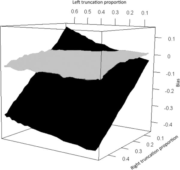
Bias of the unweighted estimator ${\widehat{\beta }}_{uw}$ (black) and nonparametric weighted estimator ${\widehat{\beta }}_{w_{np}}$ (gray). Left truncation time simulated from a c₁ Beta(θ₁, 1) distribution, right truncation time simulated from a c₂ Beta(1, θ₂) distribution, with c₁ = c₂ = 30. Here θ₁ ranges from 0.025 to 0.50 which results in a range of 5% to 65% truncation from the left, and θ₂ ranges from 0.25 to 5 which results in a range of 5% to 45% truncation from the right. The remaining settings are kept the same as in Table 1, with n = 250.

We also examined the robustness of ${\widehat{\beta }}_{w_{\widehat{\theta }}}$ under misspecification of the truncation distribution in Web Table 1. In this setting, ${\widehat{\beta }}_{w_{\widehat{\theta }}}$ was biased. Here ${\widehat{\beta }}_{w_{np}}$ still had little bias, as ${\widehat{\beta }}_{w_{np}}$ makes no distributional assumptions for the truncation times.

The simulations above assumed U and V are independent. In some cases, V can be expressed as V = U + d₀, where d₀ can be random or constant. To assess the performance of our proposed estimators under this dependent truncation structure, we conducted a simulation study (Web Table 2). The results are similar to those presented in Table 1.

5. Application to Alzheimer’s Disease Study

We illustrate our method by considering an autopsy-confirmed AD study conducted by the Center for Neurodegenerative Disease Research at the University of Pennsylvania. The target population for the research purposes of this study consists of all subjects with AD symptom onset before 2012 that met the study criteria and therefore would have been eligible to enter the center. Our observed sample contains all subjects who entered the center between 1995 and 2012, and had an autopsy performed before 2012. Thus one criterion for a subject to be included in our sample is that they did not succumb to AD before they entered the study, yielding left truncated data. In addition, our sample only contains subjects who had an autopsy-confirmed diagnosis of AD, and therefore we have no knowledge of subjects who live past the end of the study. Thus our data is also right truncated. Our data consists of n=47 subjects, all of whom have event times. The event time of interest is the survival time (T) from AD symptom onset. The left truncation time (U) is the time between the onset of AD symptoms and entry into the study (i.e. initial clinic visit). The right truncation time (V) is the time between the onset of AD symptoms and the end of the study, which is taken to be July 15, 2012. Due to double truncation, we only observe subjects with U ≤ T ≤ V .

Our motivation for studying the effect of education on survival in AD is that education serves as a proxy for cognitive reserve (CR). CR theorizes that individuals develop cognitive strategies and neuronal connections throughout their lives through experiences such as education and other forms of mental engagement (Valenzuela and Sachdev 2007). For example, CR may have a protective role in the brain, and therefore lengthen survival during the course of the disease (Ientile et al. 2013). Paradise et al. (2009) and Meng and D’Arcy (2012) failed to detect an effect of education on survival from AD symptom onset. However the studies included in their meta-analyses did not consist of populations with autopsy-confirmed AD.

Here we assess the effect of education on survival time in our autopsy-confirmed cohort, where education is measured by years of schooling. The median years of education in this cohort is 16 years. Comparing the low education group (< 16 years) and high education group (⩾ 16 years) on the variables of interest revealed no significant differences (Table 2).

Table 2.

Comparing low education (< 16 years) and high education (⩾ 16 years) groups

Variable	Low education (n=15) mean (sd)	High education (n=32) mean (sd)	Test statistic	p-value
Age Onset	61.8 (10.5)	63.2 (12.9)	t45 = −0.37	0.712
Survival time	8.7 (3.4)	7.9 (3.2)	t45 = 0.80	0.430
Time to study entry	3.4 (1.71)	2.7 (1.5)	t45 = 1.37	0.177
Time to end of study	13.3 (2.8)	12.6 (4.7)	t45 = 0.58	0.563
Male (%)	53	72	${\chi }_1^2=1.56$	0.211

Survival time, time to study entry, and time to end of study are measured in years from AD symptom onset.

Since our data is doubly truncated, we apply the Cox regression model using the proposed weighted estimating equation approach. We check the assumption of independence between the truncation and survival times in the observable region U ≤ T ≤ V using the conditional Kendall’s tau proposed by Martin and Betensky (2005). The resulting p-value is 0.10, and therefore we do not have enough evidence to reject the null hypothesis that the observed survival and truncation times are independent. We justify the identifiability constraints from Section 2.1, $a_{H_U}<a_F\le a_{H_V}$ and $b_{H_U}\le b_F<b_{H_V}$, in Web Appendix D.

We adjust for double truncation using both parametric and nonparametric weights. The parametric weights are estimated under the assumption that U ~ c₁Beta(α₁, β₁) and V ~ c₂Beta(α₂, β₂), where c₁ = 20 and c₂ = 40. Under these parametric assumptions, we have $\widehat{{\alpha }_1}=2.6$, $\widehat{{\beta }_1}=13.8$ and $\widehat{{\alpha }_2}=3.0$, $\widehat{{\beta }_2}=9.7$. To check our assumption of the beta distribution, we test the null hypothesis H₀ : K(u, v) = K_θ(u, v), where θ = (α₁, β₁, α₂, β₂). Here the parametric joint cumulative distribution function $K_{\mathbf{\theta }}(u,v)=I_{u/c_1}({\alpha }_1,{\beta }_1)\times I_{v/c_2}({\alpha }_2,{\beta }_2)$, where $I_x(a,b)={\displaystyle {\int }_0^x{t}^{a-1}{(1-t)}^{b-1}dt}$. As described by Moreira, de Ũna-Álvarez, and Van Keilegom (2014), we can test H₀ using a Kolmogorov-Smirnov type test statistic $D_n=su{p}_{u,v\in ℝ}|K_n(u,v)-K_{\widehat{\mathbf{\theta }}}(u,v)|$, where K_n(u, v) is the NPMLE of K(u, v) (Shen 2010a). This yields a p-value of 0.60, and therefore we do not have enough evidence against the beta distribution assumption for the truncation times.

Table 3 displays the results from the Cox regression model using no weights, parametric weights, and nonparametric weights. The effects of age at AD symptom onset and male on survival are nearly twice as large in the weighted models relative to the unweighted model, but these effects are only significant under parametric assumptions. When we do not account for double truncation, there is no effect of education on survival ( ${\widehat{\beta }}_{uw}=0$; 95% CI: [−0.11,0.12]). When we account for double truncation, higher education is associated with increased survival under parametric weights ( ${\widehat{\mathbf{\beta }}}_{w_{\widehat{\theta }}}=-0.07$; 95% CI: [−0.20,0.06]) and nonparametric weights ( ${\widehat{\beta }}_{w_{np}}=-0.06$; 95% CI: [−0.29,0.19]). However the confidence intervals for both ${\widehat{\beta }}_{w_{\widehat{\theta }}}$ and ${\widehat{\beta }}_{w_{np}}$ contain 0.

Table 3.

Application results of Cox regression model. Event time is years from AD symptom onset to death.

Predictor	Unweighted ${\widehat{\beta }}_{uw}(\widehat{\text{SE}})$	95% CI	Parametric weights ${\widehat{\beta }}_{u{w}_{\widehat{\theta }}}(\widehat{\text{SE}})$	95% CI	Nonparametric weights ${\widehat{\beta }}_{w_{np}}(\widehat{\text{SE}})$	95%CI
Age Onset	0.03 (0.03)	(−0.01, 0.06)	0.05 (0.02)	(0.00, 0.09)	0.05 (0.03)	(−0.02, 0.12)
Male	0.45 (0.34)	(−0.21, 1.11)	1.01 (0.49)	(0.06, 1.97)	0.95 (0.61)	(−0.36, 2.18)
Education	0.00 (0.06)	(−0.11, 0.12)	−0.07 (0.07)	(−0.20, 0.06)	−0.06 (0.11)	(−0.29, 0.19)

6. Discussion

We proposed a weighted estimating equation approach to adjust the Cox regression model under double truncation, by weighting the subjects in the score equation of the Cox partial likelihood by the inverse of the probability that they were observed (i.e. not truncated). The probability of being observed was estimated both parametrically and nonparametrically by methods introduced in Shen (2010a, 2010b) and Moreira and de Ũna-Álvarez (2010), and did not require any contribution from missing subjects. The proposed hazard ratio estimators are consistent. The simulation studies confirmed that the proposed estimators have little bias, while the naïve estimator which ignores truncation is biased. The parametric weighted estimator is asymptotically normal, and a consistent estimator of its asymptotic variance is provided. Our simulations showed that the bootstrap estimate of the standard error for the nonparametric weighted estimator matched the observed sample standard deviation.

The proposed estimators have little bias in practical settings, which has useful implications in observational studies. One example is AD - a severe neurodegenerative disorder which has devastating effects for patients and their caregivers. Thus any knowledge of factors associated with extending survival from AD symptom onset can have a great impact on society. In this paper, we assessed the effect of education on survival in subjects with autopsy-confirmed AD. Our method is critical for analyzing data of this sort, since autopsy confirmation leads to doubly truncated survival times, which can result in biased hazard ratio estimators. While AD studies that do not use autopsy confirmation avoid double truncation, the conclusions based on these studies may be unreliable due to the inaccuracy of clinical diagnosis. This may explain the inconclusive findings of the two meta-analyses conducted by Paradise et al. (2009) and Meng and D’Arcy (2012), who used studies with clinically diagnosed AD subjects to examine the effect of education on survival. Using our proposed method on an autopsy-confirmed AD study found that higher education was associated with increased survival. However, these effects were not statistically significant. This may be due to our small sample size and the fact that our sample was highly educated (range = 12 – 20 years). When double truncation was ignored, we found no effect of education on survival.

The consistency of the estimated selection probabilities used in our proposed method rests on the assumption of independence between the survival and truncation times in the observable region. A violation of this assumption may lead to biased hazard ratio estimators. Currently, we are not aware of any methods to adjust for violations of this assumption. Because the estimation procedure for the selection probabilities does not make use of the assumed relationship between the survival time and covariates, this independence assumption cannot be relaxed simply by covariate adjustment in the Cox model. However, when conditional independence on discrete covariates holds, we can stratify the data based on the levels of the covariates, and then estimate the weights independently within each stratum. In this situation, conditional independence can be tested by applying the conditional Kendall’s tau (Martin and Betensky 2005) within each stratum. However, this approach may not be practical if the number of strata is large. Future work is thus needed to relax the independence assumption.

Currently there are no closed form estimates for the nonparametric selection probabilities, which complicate the development of asymptotic properties for the nonparametric weighted estimator. While our simulations show that the nonparametric weighted estimator appears to satisfy asymptotic normality, an extension to our method is to formally prove this result. Furthermore, the theoretical validity of the bootstrap estimators needs to be established. Finally, the proposed method assumes that no censoring is present in the data. While right censoring is uncommon under double truncation, interval censoring could be present in the data (Bilker and Wang 1996, Martin and Betensky 2005). Future work would thus be needed to extend our methods in the presence of interval censored data.

While weighting leads to consistent estimators, it may also lead to an increase in the variance of these estimators in certain cases. In practice, an investigator may wonder whether it is worth adjusting for double truncation. We recommend using the proposed weighted estimators since they are consistent and perform well in finite samples, while the naïve estimator can be biased even in cases of mild truncation. When the truncation is severe, the naïve estimator can be heavily biased. However, severe truncation may produce large weights which can lead to an increase in the standard error of the weighted estimators. Therefore if the estimated weights are large, we recommend performing a sensitivity analysis by truncating the weights as described in Seaman and White (2013).

References

- Beach TG, Monsell SE, Phillips LE, Kukull W. Accuracy of the Clinical Diagnosis of Alzeimer Disease at National Institute on Aging Alzheimer’s Disease Centers, 2005–2010. Journal of Neuropathology & Experimental Neurology. 2012;71:266–273. doi: 10.1097/NEN.0b013e31824b211b. [DOI] [PMC free article] [PubMed] [Google Scholar]
- Bilker WB, Wang MC. A Semiparametric Extension of the Mann-Whitney Test for Randomly Truncated Data. Biometrics. 1996;52:10–20. [PubMed] [Google Scholar]
- Binder D. Fitting Cox’s proportional hazards models from survey data. Biometrika. 1992;79:139–147. [Google Scholar]
- Cox DR. Regression Models and Life-Tables. Journal of the Royal Statistical Society Series B (Methodological) 1972;34:187–220. [Google Scholar]
- Efron B, Petrosian V. Nonparametric Methods for Doubly Truncated Data. Journal of the American Statistical Association. 1999;94:824–834. [Google Scholar]
- Efron B, Tibshirani RJ. An Introduction to the Bootstrap. Chapman & Hall; 1993. [Google Scholar]
- Ientile L, De Pasquale R, Monacelli F, Odetti P, Traverso N, Cammarata S, Tabaton M, Dijk B. Survival rate in patients affected by dementia followed by memory clinics (UVA) in Italy. Journal of Alzheimer’s Disease. 2013;36:303–309. doi: 10.3233/JAD-130002. [DOI] [PubMed] [Google Scholar]
- Kalbfleisch JD, Lawless JF. Regression models for right truncated data with application to AIDS incubation times and reporting lags. Statistica Sinica. 1991;1:19–32. [Google Scholar]
- Lai TL, Ying Z. Rank regression methods for left-truncated and right-censored data. The Annals of Statistics. 1991;19:531–556. [Google Scholar]
- Lin D. On fitting Cox’s proportional hazards models to survey data. Biometrika. 2000;87:37–47. [Google Scholar]
- Martin EC, Betensky RA. Testing Quasi-Independence of Failure and Truncation Times via Conditional Kendall’s Tau. Journal of the American Statistical Association. 2005;100:484–492. [Google Scholar]
- Meng X, D’Arcy C. Education and dementia in the context of the cognitive reserve hypothesis: A systematic review with meta-analyses and qualitative analyses. PLoS ONE. 2012;7 doi: 10.1371/journal.pone.0038268. [DOI] [PMC free article] [PubMed] [Google Scholar]
- Moreira C, de Ũna Álvarez J. A semiparametric estimator of survival for doubly truncated data. Statistics in Medicine. 2010;29:3147–3159. doi: 10.1002/sim.3938. [DOI] [PubMed] [Google Scholar]
- Moreira C, de Ũna Álvarez J, Meira-Machado L. Nonparametric regression with doubly truncated data. Computational Statistics and Data Analysis. 2016;93:294–307. [Google Scholar]
- Moreira C, de Ũna Álvarez J, Van Keilegom I. Goodness-of-fit tests for a semiparametric model under random double truncation. Computational Statistics. 2014;29:1365–1379. [Google Scholar]
- Pan Q, Schaubel DE. Proportional hazards models based on biased samples and estimated selection probabilities. Canadian Journal of Statistics. 2008;36:111–127. [Google Scholar]
- Paradise M, Cooper C, Livingston G. Systematic review of the effect of education on survival in Alzheimer’s disease. International Psychogeriatrics/IPA. 2009;21:25–32. doi: 10.1017/S1041610208008053. [DOI] [PubMed] [Google Scholar]
- Seaman SR, White IR. Review of inverse probability weighting for dealing with missing data. Stat Methods in Medical Research. 2013;22:278–295. doi: 10.1177/0962280210395740. [DOI] [PubMed] [Google Scholar]
- Shen PS. Nonparametric analysis of doubly truncated data. Annals of the Institute of Statistical Mathematics. 2010a;62:835–853. [Google Scholar]
- Shen PS. Semiparametric analysis of doubly truncated data. Communications in Statistics-Theory and Methods. 2010b;39:3178–3190. [Google Scholar]
- Shen PS. Regression analysis of interval censored and doubly truncated data with linear transformation models. Computational Statistics. 2013;28:581–596. [Google Scholar]
- Turnbull BW. The empirical distribution function with arbitrarily grouped, censored and truncated data. Journal of the Royal Statistical Society, Series B. 1976;38:290–295. [Google Scholar]
- Valenzuela MJ, Sachdev P. Assessment of complex mental activity across the lifespan: development of the Lifetime of Experiences Questionnaire (LEQ) Psychological Medicine. 2007;37:1015–1025. doi: 10.1017/S003329170600938X. [DOI] [PubMed] [Google Scholar]
- Wang MC. Hazards regression analysis for length-biased data. Biometrika. 1996;83:343–354. [Google Scholar]
- Woodroofe M. Estimating a distribution function with truncated data. Annals of Statistics. 1985;13:163–177. [Google Scholar]
Associated Data
This section collects any data citations, data availability statements, or supplementary materials included in this article.