Multiple Consecutive Recapture of Rigid Nanoparticles Using a Solid-state Nanopore Sensor

Abstract

Solid-state nanopore sensors have been used to measure the size of a nanoparticle by applying a resistive pulse sensing technique. Previously, the size distribution of the population pool could be investigated utilizing data from a single translocation, however, the accuracy of the distribution is limited due to the lack of repeated data. In this study, we characterized polystyrene nanobeads utilizing single particle recapture techniques, which provide a better statistical estimate of the size distribution than that of single sampling techniques. The pulses and translocation times of two different sized nanobeads (80 nm and 125 nm in diameter) were acquired repeatedly as nanobeads were recaptured multiple times using an automated system controlled by custom-built scripts. The drift-diffusion equation was solved to find good estimates for the configuration parameters of the recapture system. The results of the experiment indicated enhancement of measurement precision and accuracy as nanobeads were recaptured multiple times. Reciprocity of the recapture and capacitive effects in solid state nanopores are discussed. Our findings suggest that solid-state nanopores and an automated recapture system can also be applied to soft nanoparticles, such as liposomes, exosomes, or viruses, to analyze their mechanical properties in single-particle resolution.

1. INTRODUCTION

Nanopore-based resistive pulse sensing is a highly sensitive technique that is based on the principle that the translocation of a nanoparticle through a nanopore causes a resistive pulse in the measured electrical current. Nanopore sensors have been used to analyze various analytes such as biomacromolecules [1–6], rigid [7, 8], and deformable particles [9–11]. Rigid nanoparticles are good drug carriers for transdermal or cancer drug delivery, due to the faster cellular internalization when compared to soft particles [12–15]. Thus, it is crucial to measure rigid nanoparticles’ size and mobility accurately for the success of drug delivery applications with rigid nanoparticles.

It is possible to obtain single particle information using nanopore sensors for a measurement, while other techniques to characterize single nanoparticles, such as dynamic light scattering [16] and X-ray analysis [17], provide information that depends on the ensemble measurements of nanoparticles at each measurement. Since nanopore sensors can measure single particle properties, such as translocation time and peak size, with a single measurement, it is also possible to conduct population analysis on diluted nanoparticle suspensions [9, 10]. However, statistically, a single measurement per particle is not reliable for accurate knowledge of the size and mobility of nanoparticles. To achieve a higher level of accuracy, it is imperative that sufficient translocation data is gathered from a nanoparticle. For this purpose, recapture systems have been developed where a single particle is translocated multiple times while resistive pulse data is collected repeatedly. Until recently, nanopore recapture systems have been adopted to recapture relatively large and long DNA strands [18]. The DNA translocation induces a larger and longer resistive pulse in the baseline current than that of rigid nanoparticles; this enabled experimentalists to successfully recapture DNA more than 1000 times consecutively [19]. Rigid nanoparticle recaptures, however, have not been reported yet to the knowledge of the authors.

In this study, the resistive pulses and the translocation times of two different polystyrene nanobeads are analyzed. Pulse and translocation time information was collected when rigid nanoparticles translocated multiple times through the nanopore in the recapture experiments. Recapture experiments were performed to accurately measure the resistive pulse and translocation time of the two particles using in-house computer algorithms. Statistical analysis was performed to understand the refinement made by performing recapture on single particles. Lastly, several observations and limitations were reported with a nanopore sensor, based on the analysis of recaptured nanoparticles.

2. MATERIALS AND METHODS

2.1 Nanoparticle preparation

Spherical polystyrene nanobeads of 80 nm and 125 nm were purchased (Polysciences, Warrington, PA) and subsequently scanned with a transmission electron microscope (JEM-2100F, JEOL, Figure 1a). For the experiments, the particles were diluted to 10⁻⁵ g/ml in a buffer solution of 50 mM KCl and 20 mM phosphate buffer (pH 6). Care was exercised to keep the particle suspension colloidally stable during the translocation experiments, meaning nanoparticles were well dispersed in the buffer solution without aggregation. Chemical and mechanical methods were used to prepare the solution. Triton X-100 was added at a concentration of 0.015 % to disperse the nanoparticles in the solution. KCl and phosphate salt concentration were controlled since high salt concentration accelerated the particle aggregation due to hydrophobic interactions [20]. The nanoparticle suspension was treated in an ultrasonic bath for 30 minutes before each experiment [21]. Dynamic light scattering experiments were employed to measure the size distribution of the particles in the buffer solution [16]. These experiments indicated no aggregation in the particle suspension (Figure 1b).

Figure 1.

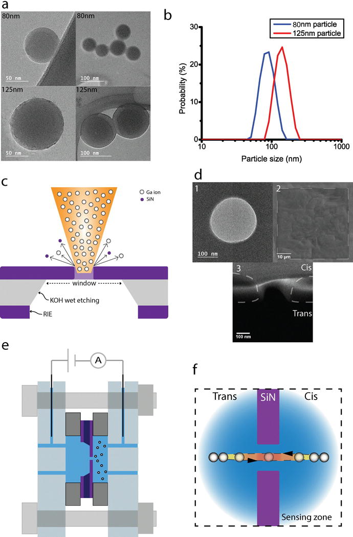
(a) TEM pictures of 80 nm and 125 nm polystyrene nanobeads. (b) Histogram for hydrodynamic diameter of 80 nm and 125 nm polystyrene nanobeads; measurement using Zetasizer Nano ZS, Malvern with pH 6 Phosphate buffer solution. (c) A schematic figure representing fabrication procedures of the SiN membrane and the nanopore. (d) 1) TEM picture of 250 nm diameter nanopore. 2) SEM picture of 50 μm square SiN window. 3) SEM picture of pore cross section at the pore central axis. (e) A schematic figure of the assembly of the flow cell and the nanopore chip. (f) A schematic figure of the nanoparticle recapture event.

2.2 Nanopore fabrication and preparation

200 nm of a low-stressed silicon nitride (Si_xN_y) membrane was deposited on both sides of a 4-inch silicon wafer of 525 μm thickness using the low pressure chemical vapor deposition method. A 50 μm square silicon nitride window was made on the silicon wafer through microfabrication procedures of photolithography, reactive ion etching, and KOH wet etching. Figure 1c shows a schematic of the etched wafer and the nanopore. A 250 nm diameter pore was fabricated using a dual-beam focused ion beam (DB-FIB, Helios Nanolab, FEI) in the 50 μm window [1, 22]. In Figure 1d, electron microscopy micrographs of the nanopore are given. Each pore was fabricated in 7 seconds with 30 kV of acceleration voltage and 10 pA of current. Each fabricated nanopore was examined using electron micrographs, since small deformations at the nanopore edges deteriorated the quality of the translocation experiments. The third inset figure in Figure 1d shows the scanning electron micrographs of the nanopore cross section, where the chamfer at the rim of the nanopore is evident. The pore length (200 nm, SiN membrane thickness) was confirmed using this figure.

Before the experiments, nanopore chips were cleaned using the Piranha solution for 10 minutes at 80 °C [23]. The pertinent cleaning of nanopores is important, first, to enhance the hydrophilicity of the pore for proper conductance [24–26], and second, to clean the nanopore free of debris, which could mechanically interrupt the translocation events. For the nanopore cleaning, the safety protocol suggested by the Environmental Health and Safety Department of Southern Methodist University was followed. After the cleaning, the chip was rinsed with deionized water three times.

2.3 Experimental setup

The flow cell that was used to house the nanopore consists of Cis and Trans chambers. A schematic of the assembled flow cell is shown in Figure 1e. The nanopore is positioned between the two chambers, where polydimethylsiloxane (PDMS) gaskets with an inner diameter of 3 mm separate the nanopore from the chambers. Inlet and outlet holes were drilled on the polycarbonate housing. A separate pair of inserts was used to hold a pair of Ag/AgCl electrodes. These Ag/AgCl electrodes were fabricated by soaking a 0.25 mm diameter Ag wire in bleach (Clorox) for 30 minutes. A new set of Ag/AgCl electrodes were used for every experiment, since the AgCl layer was easily worn during experiments, which could seriously exacerbate the probe sensitivity. Care was taken to avoid any bubble formation in the chambers since small bubbles could disturb or block the current. In order to facilitate the filling of the chamber, the PDMS gaskets were exposed to O₂ plasma for 3 minutes, enhancing the wetting behavior of the PDMS gasket surface. The nanoparticle suspension was introduced into the Cis chamber while the Trans chamber did not contain any nanoparticles.

Operation Principle

The schematic in Figure 1f shows the operation principle of the experimental setup. An electric field was generated inside the chamber as the electrodes were energized at a fixed electric potential. The electric field in the flow cell was simulated using a commercial solver (COMSOL Multiphysics), and given in Figure 2a. As shown in the figure, the electric field was locally amplified in the nanopore due to the strong nanopore resistance, which caused the sudden potential drop. As a result of the interaction between the electric field and the particle charge, nanoparticles experience electrophoretic motion. Electroosmosis and dielectrophoresis are the two other mechanisms that govern particle motion. Particles could travel either to the anode or to the cathode depending on their zeta potential [27]. In Figure 2b, the nanoparticle zeta potential, which was measured using dynamic light scattering at pH values of 6, 7, and 8, is given. The particle translocation experiments were conducted at pH 6, where the particle zeta potential was negative. The direction of particle movement in the flow cell was, therefore, from the anode to the cathode. While a nanoparticle was entering the sensing zone (Figure 1f), the recorded current exhibited a sharp decrease (Figure 2c). Analyzing this change in the measured current signal, particle properties could be inferred from signal parameters such as translocation time and peak size.

Figure 2.

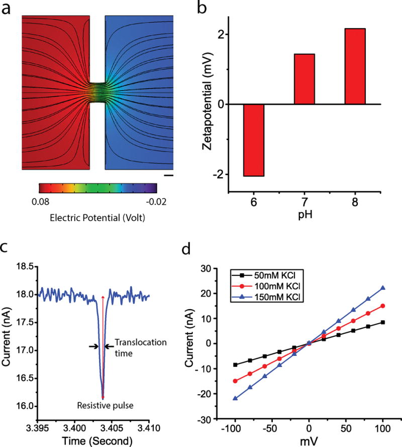
(a) The electric field simulation around the nanopore. Scale bar: 100 nm. (b) Zeta-potential measurement using Zetasizer nano ZS, Malvern at pH 6, 7, and 8. The zeta potential of the 125 nm polystyrene beads was measured in phosphate buffers. (c) A single peak in a resistive pulse that is marked for the peak size and the translocation time at the full width at half maximum (FWHM). (d) Pore conductance test using KCl solutions of 50 mM, 100 mM, and 150 mM.

Data acquisition

Two electrodes connected the two electrolyte chambers to an amplifier (Axopatch 200B, Molecular Devices), which applied voltage to the electrodes and recorded the resulting current signal from the system. The current signal was processed with a digitizer (Digidata 1440A, Molecular Devices) for the pore conductance tests (Figure 2d) or using a data acquisition board (BNC-2110, National Instrument) with a PCI card (PCI 6259, National Instrument). The data acquisition board was used for recapture experiments since the board allowed us to modulate the polarity of the applied voltage using LabVIEW script. The current data was acquired at 30 kHz sampling frequency and filtered by a 2 kHz Bessel filter. The recorded data was analyzed using a custom-made MATLAB (MathWorks, MA) code. The function of the 2 kHz Bessel filter was to achieve a higher signal-to-noise ratio, which also facilitated the detection of resistive pulses in the measured signal without any loss.

2.4 Automatic feedback control recapture system

A LabVIEW (National Instruments, TX) script was developed to enable multiple recaptures of nanoparticles. The script constantly reads the current (I) from the data acquisition system and averages the recorded current at 1.67 ms windows. The script automatically changes the polarity of the applied voltage after a translocation event to achieve recapture of a particle. The following inequality is used to detect the translocation events, which is necessary for recapture.

$$I_i^k<{\overline{\mathit{I}}}_{i-1}-\alpha \ast \tau .$$ (1)

In the above equation indexes i and k are for the moving average windows and the data points in the averaging windows, respectively. ${\overline{\mathit{I}}}_{i-1}$ is the average current at the $i-1$ window, τ is the peak-to-peak noise, and α is a factor, which is manually set. The script recognizes an event as a particle translocation if the current data ( $I_i^k$) deviates more than “α * τ” away from the previous baseline ( ${\overline{\mathit{I}}}_{i-1}$).

The nanopore sensor forms an RC circuit, where the electric charge builds up at the silicon nitride layer and causes the capacitance effect (Figure 3a). Due to the effect, there is an exponential decrease in the current baseline, which is characterized by the settling time ( $T_{\mathit{settle}}$ in Figure 3b). As the voltage polarity is reversed in the recapture experiment, the translocation event could occur during the exponential decay of the current. In this case, the detection of the translocation event becomes difficult. To avoid the recapture event to be hidden under the exponential current decay, the voltage reversal is delayed by a certain time ( $T_{\mathit{delay}}$ in Figure 3b) after the detection of a translocation event, which eventually increased the recapture time ( $T_{\mathit{recapture}}$ in Figure 3b). This allowed the particle to avoid the exponential current decay and to be recaptured consecutively. In addition, the peak detection algorithm was disabled during the decay to prevent the script from falsely reversing the voltage polarity due to the steep current baseline ( $T_{\mathit{skip}}$ in Figure 3b). Using this strategy, single particle recaptures were successfully conducted with high accuracy and reliability.

Figure 3.

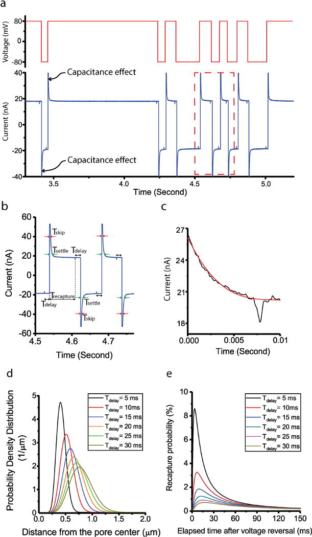
(a) Multiple consecutive recapture events of single 125 nm nanoparticle. The above red line shows the applied voltage during the experiment. (b) Enlarged picture of the red box in Figure 3a. $T_{\mathit{delay}}$ is the period between peak detection and voltage reversal. $T_{\mathit{skip}}$ is the period when peak detection function of LabView system is disabled to avoid the capacitance effect. $T_{\mathit{settle}}$ is the period of exponential decrease of the current baseline after voltage reversal. $T_{\mathit{recapture}}$ is the period between voltage reversal and next peak detection. (c) Third order polynomial fitting for the peak characterization on the current baseline. (d) Probability density distribution with different $T_{\mathit{delay}}$ for 125nm nanoparticles. (e) Recapture probability with different $T_{\mathit{delay}}$ for 125nm nanoparticles.

2.5 Data analysis

For the current data with non-recaptured particles, we corrected the current baseline fluctuations by the moving average method and properly determined the peak size by iterative method, which was reported by Plesa and Dekker [28]. For the current data with recaptured particles, the identification of the translocation events was more complex, since a large number of particles got recaptured during a gradually settling current baseline (not during the beginning stage of exponential decrease) and the moving window method was no longer suitable for such scenarios. In this case, we located the translocation events using the peak detection method in the LabVIEW script and determined if the translocation event was happening on a stable current baseline. For the events on a stable current, we used the iterative method to characterize them. For the events on the settling current, we combined a third-order polynomial fitting (Figure 3c) with the iterative method, to remove the influence of the peak on the fitting. Each time after we fit the current data, we replaced the data points which deviated more than τ (peak-to-peak noise) away from the fitting baseline with the data points in the polynomial function. This fitting process lasted for three iterations, which was empirically proven to be enough to properly determine the peak size. A third-order polynomial fitting was used for the inherently exponentially settling current because only 10 ms of current data around the translocation event was investigated, which was too short for the exponential function to achieve a good fitting. The translocation time of both non-recaptured and recaptured particles was extracted using the full width at half maximum (FWHM) method [29].

2.6 Population pool analysis

The pooled mean and the pooled standard deviation formulas were applied to the experimental data. The pooled mean and the standard deviation of an ensemble measurement made on M particles are given by the following equations, respectively,

$$\langle \overline{x}\rangle =\frac{{{\displaystyle \sum }}_{j=1}^M{N}_j{\overline{x}}_j}{{{\displaystyle \sum }}_{j=1}^M{N}_j},$$ (2)

$$\langle s_x\rangle =\sqrt{\frac{{{\displaystyle \sum }}_{j=1}^M{v}_j{s}_{x_j}^2}{{{\displaystyle \sum }}_{j=1}^M{v}_j}}$$ (3)

In the above equations, x is for particle data (peak size or translocation time), $\overline{x}$ is an average performed over $N_j$ successive recaptures, where index j is for different particles, and $v_j$ is the degrees of freedom.

2.7 Drift diffusion equation

The dimensionless form of the drift diffusion equation was solved to estimate a proper $T_{\mathit{delay}}$ [18].

$$\frac{\partial c\left(r_1,s\right)}{\partial s}=\frac{1}{r_1^2}\frac{\partial }{\partial r_1}\left(\mp c\left(r_1,s\right)+r_1^2\frac{\partial c\left(r_1,s\right)}{\partial r_1}\right),$$ (4)

where s is the dimensionless time, $r_1$ = $r/L$ is a dimensionless radial coordinate, with radial distance r from the pore center and characteristic length L. The characteristic length in the above equation is the recapture distance $L_c$ (1740.9 nm for 125 nm particles, 1044.5 nm for 80 nm particles), beyond which the electrophoretic velocity is smaller than the diffusion velocity. ‘−’ is for the electrophoretic motion away from the pore while ‘+’ means the opposite, and c is the volume density of the particle, which is related to the probability density function p using the following equation,

$$p=2\pi r^{2}c\left(r\right).$$ (5)

Using the above equations, we were able to compute the probability density distribution of particles at any time before and after the voltage reversal.

The following parameters were used for the solution of the drift diffusion equation with 125 nm particles: particle zeta potential ζ = −2 mV, viscosity of the buffer solution η = ${10}^{-3}Pa·s$, electrophoretic mobility of the particle $\mu =1.4166\times {10}^{-9}{m}^2{V}^{-1}{s}^{-1}$, temperature T = 298 K, conductivity of the solution $\sigma =1.6S/m$, and diffusion constant of the polystyrene particles $D=1.6189\times {10}^{-12}{m}^2{s}^{-1}$, which was obtained from a previous study [30]. For brevity, the parameters and simulation results for 80 nm particles are not shown in this paper. The solution of the above equation was verified using benchmark data [18].

2.8 COMSOL simulation

Finite element simulation using a commercial software COMSOL Multiphysics were employed for the electric field calculations in Figure 2a [31]. The 2D axisymmetric computation domains (Cis and Trans chambers) were 2000 nm in diameter and 2000 nm in length, and the pore in the domain was 250 nm in diameter and 200 nm in length. Our computational model consisted of coupled Poisson, Nernst Planck, and Navier-Stokes equations enabled to simulate all the physical phenomena in the nanopore system. The locally amplified electric field was clearly illustrated by the denser electric field streamlines near the pore. 0.103 M KCl solution was used in the simulations to match the pore conductance in the experiment. An electric potential of 80 mV was applied for the simulation, which was the same voltage used for all experimental conditions. The other parameters we used for the COMSOL simulations were: diffusion constant of $K^{+}{D}_K=1.975\times {10}^{-9}{m}^2/s$, diffusion constant of $C{l}^{-}$ $D_{Cl}=2.032\times {10}^{-9}{m}^2/s$, membrane surface charge density $-20mC/m^2$, temperature $T=293.15K$, and viscosity of the solution $\mu ={10}^{-3}Pa·s$.

3. RESULTS AND DISCUSSION

3.1 Conductance of the nanopore

Prior to the nanoparticle translocation experiments, the pore conductance tests were done to confirm the pore quality. The pore conductance was measured in the flow cell using 50 mM, 100 mM, and 150 mM KCl solutions without the nanoparticles. In these measurements, the current was measured as voltage was varied between −100 mV to 100 mV with 25 mV steps. The results are given in Figure 2d. As the concentration of salt gets higher, the pore conductance increases allowing a larger current flow through the nanopore. The measured pore conductance using the data of the 100 mM KCl solution was 150.35 nS, which is close to the value from the analytical calculation. Assuming the pore as an empty cylinder, an analytical estimate of the conductance could be calculated using the following equation [7],

$$G=\frac{1}{R_{\mathit{pore}}+R_{\mathit{acc}}}=\frac{\pi \sigma D^2}{4L+\pi D},$$ (6)

where D and L are pore diameter and pore length, σ is the conductivity of the solution, $R_{\mathit{pore}}$ and $R_{\mathit{acc}}$ are the geometrical resistance and access resistance of the pore, respectively. Since the pore length (200 nm) and diameter (250 nm) have similar values, the access resistance contributes to nearly half of the overall resistance. The experimentally measured value of the pore conductance is 5.16 % lower than the theoretical value of 158.53 nS. This small difference between experimental and theoretical results could be due to the asymmetric geometry of the nanopore, and to the resistive effects of the electrode polarization.

3.2 Recapture probability

Recapture kinetics were studied by computer simulation. In Figure 3d, the probability density distribution of 125 nm polystyrene nanobeads is shown for different delay times. The location of the peak in the probability density function moves away from the pore center due to the electrophoretic force as a function of the delay time. To find the recapture probability after the voltage reversal with a certain delay time, the area under the probability density curve is integrated from the origin to a distance of 250 nm, which is the diameter of the particle plus the half length of the pore. It is assumed that the particles could be recaptured by 100 % chance within 250 nm radial distance from the pore center. Figure 3e shows that the highest recapture probability for 125 nm particles drastically drops from 8.60 % to 0.71 %, while the delay time increases from 5 ms to 30 ms. Such estimation of recapture probability offered a theoretical background to properly choose the key parameters for the recapture experiment. For example, we chose the delay time between 5 ms and 20 ms in the experiment, since further increase in delay time would result in extremely low recapture probability.

3.3 Recapture experiment

We succeeded at consecutive multiple recaptures of single particles during the recapture experiments. Representative traces of the recorded current of 80 nm and 125 nm single particles were shown in Figure 3a and Figure 4a–4c. In these figures, as a translocation was identified by the system, the voltage polarity was automatically reversed after a certain delay time. The current baseline after the settling time in Figure 4c was about 21 pA, which was higher than the current baseline of Figure 4a and 4b. This was because a higher phosphate buffer concentration was used for the 80 nm particle recapture experiment in Figure 4c. Recapture data from nine individual 125 nm particles is given in Figure 4d, where the average current drop is plotted for each particle with its standard deviation. The small standard deviation of each set demonstrated that we consecutively captured the same particles. To be specific, the averaged standard deviation value was 0.129, which was about one third of the standard deviation 0.383 of the population pool.

Figure 4.

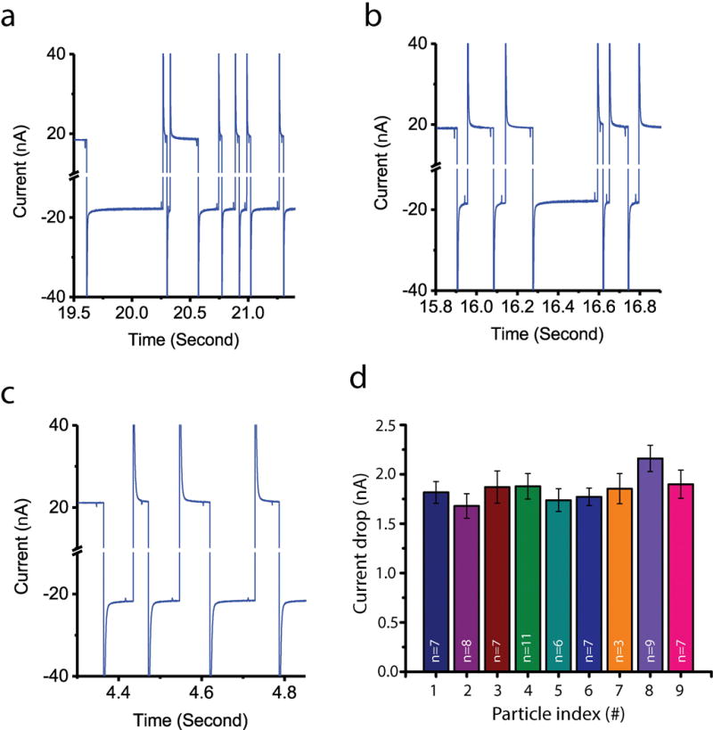
Recapture data and single particle analysis (a) Recapture experiment data with 125nm bead. $T_{\mathit{delay}}$: 12.5 ms, $T_{\mathit{skip}}$: 12 ms, 15 mM pH 6 phosphate buffer with 50 mM KCl. (b) Recapture experiment data with 125 nm bead. $T_{\mathit{delay}}$: 12.5 ms, $T_{\mathit{skip}}$: 12 ms, 15 mM pH 6 phosphate buffer with 50 mM KCl (same experimental condition with figure 4a). (c) Recapture experiment data with 80 nm bead. $T_{\mathit{delay}}$: 15 ms, $T_{\mathit{skip}}$: 15ms, 20 mM pH 6 phosphate buffer 50 mM KCl. (d) Bar chart for single particle analysis by comparing nine sets of recapture events from nine nanoparticles.

After testing its feasibility for single particle analysis, the peak size and translocation time distributions of single translocation and recapture data were calculated. The comparison of translocation time and peak size distribution is given in Figure 5 for 80 nm and 125 nm particles. Figure 5a–5d show the peak size and translocation time for 80 nm and 125 nm particles. Shown in the figure is the pooled mean and its standard deviation that are weighted by the recapture times. Results for 80 nm particles in Figure 5 indicated that there was a significant decrease of standard deviation in the recapture data (peak size and translocation time) when compared to the single translocation data. Accordingly, multiple recaptures increased the precision of the measurement made by the nanopore system for 80 nm particles. For 125 nm particles, on the other hand, no such significant reduction was evident in the peak size and translocation time data. The possible explanation for the size dependency is discussed on the section 3.4 and 3.5. Assuming the pore is of cylindrical shape, the relative excluded volume (χ, defined as the relative volume excluded by the particle in the pore) is [7]

$$\chi =\frac{2D_{\mathit{particle}}^3}{3L_{\mathit{pore}}{D}_{\mathit{pore}}^2},$$ (7)

which is valid only when $D_{\mathit{particle}}$≤ $L_{\mathit{pore}}$. It can be deduced that the current blockade is proportional to the cube of the particle diameter ( $\mathrm{\Delta }I~\chi ~D_{\mathit{particle}}^3$). Therefore, according to the above equation, the ratio of the peak sizes for 80 nm and 125 nm particles is 3.8147. Experimentally, the peak size ratio for recapture and single translocation data is 3.9384 and 4.2427, respectively. The data with recaptured particles thus provided a closer match to the estimate for the peak size ratio predicted by equation (7). The refinement of the nanopore measurements with recapture, therefore, not only increased precision of the measurement but also exhibited a closer match with the theory.

Figure 5.

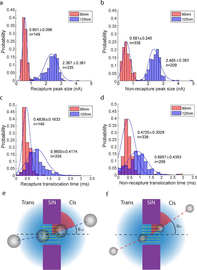
Histograms of peak size and translocation time of 80 nm and 125 nm nanoparticle population pool with a Gaussian fitting. The mean and standard deviation values in the figures are calculated based on the pooled population analysis. (a) Histogram of peak sizes of 80 nm and 125 nm nanoparticles using the recapture data. (b) Histogram of peak sizes of 80 nm and 125 nm nanoparticles using the single translocation data. (c) Histogram of translocation times of 80 nm and 125 nm nanoparticles using the recapture data. (d) Histogram of translocation times of 80 nm and 125 nm nanoparticles using the single translocation data. (e) A schematic figure for the access angle effect of 125 nm nanoparticle. (f) A schematic figure for the access angle effect of 80 nm nanoparticle.

3.4 Size dependency of the recapture event

There are a few possible reasons to explain the size dependency of the recapture data. The access angle effect is the first one, which affects the translocation time depending on the particle and pore size. Figure 5e and 5f show that the 125 nm diameter particle has a smaller maximum access angle ( ${\theta }_{125})$, which is defined by the intersection angle between the trajectory and the pore axis, than that of the 80 nm particle $\left({\theta }_{80}\right)$. If the particle is out of the maximum access angle, it has a higher chance to collide with the wall of the pore and change its trajectory inside the pore, which eventually makes the particle stay longer inside the pore and increases the translocation time. The access angle of the 80 nm (θ₈₀, 88 nm at the distribution peak) and the 125 nm (θ₁₂₅, 140 nm at the distribution peak) are 39° and 28.8° respectively. The area out of the access angle zone (90°- θ, red area of Figure 5e and 5f) can be regarded as the area from which the particle moves toward the pore and collides with the wall. If we hypothesize that the particles around the pore have the same chances to access the pore, 125 nm particles have a 68 % (61.2°/90°*100 %) probability to collide with the wall of the pore, which is 11.3 % higher than that of 80 nm particles. This access angle effect eventually makes it much more likely for the 125 nm particle to collide with the wall of the nanopore and spend more time within it during the translocation. On top of that, the number of collisions of the translocating particle is increased by the asymmetric geometry of the nanopore, which will be further discussed in section 3.5.

3.5 Reciprocity of the recapture event

The recapture and non-recapture (single translocation) events from 80 nm and 125 nm polystyrene nanobeads were recorded, and the data population was divided into two sub-populations that were based on the direction of the translocation, namely Cis to Trans and Trans to Cis. Using statistical analysis, Cis to Trans events and Trans to Cis events were compared with regards to peak size (Figure 6a) and translocation time (Figure 6b). In case of 80 nm particles, there was no significant difference between Cis to Trans and Trans to Cis in peak size and translocation time. For 125 nm particles, however, a significant difference was observed in translocation time, where Cis to Trans translocation took about one-half longer than Trans to Cis on average. To further prove the observation, the Welch’s test [32] was performed. The t value was 5.9770, which was sufficient to show the statistical significance at a level of 0.05.

Figure 6.

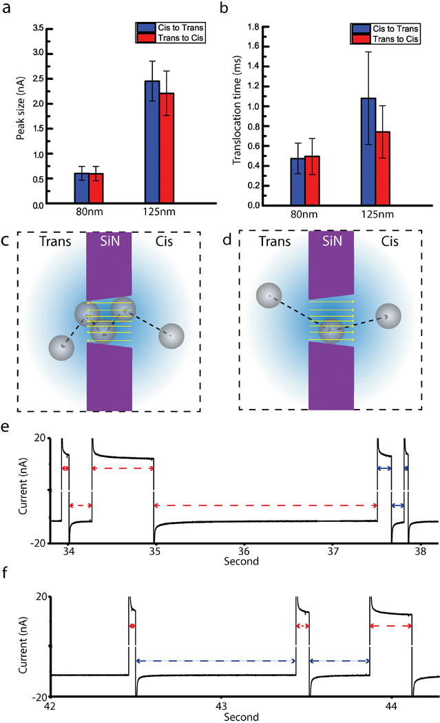
(a) Bar chart for peak sizes of Cis to Trans and Trans to Cis translocation events. (b) Bar chart for translocation times of Cis to Trans and Trans to Cis translocation events. (c) A schematic figure of the asymmetric pore geometry for the Cis to Trans translocation. (d) A schematic figure of the asymmetric pore geometry for the Trans to Cis translocation. (e) Current trace in a recapture experiment of 125 nm polystyrene nanoparticle. Recapture zone increased and then decreased both in Cis and Trans chambers. (f) Current trace in a recapture experiment of 125 nm polystyrene nanoparticle. Recapture zone increased in Cis chamber, but decreased in Trans chamber.

A possible explanation for the translocation time imbalance is that the asymmetrical pore geometry makes the translocation time different according to the direction. The pore geometry is not completely cylindrical across the pore axis, and could be regarded as a truncated cone shape (Figure 1d–3), the bottom surface of which becomes a Cis to Trans translocation entrance. Since the entrance of Cis to Trans translocation has a larger area than that of Trans to Cis, the particle enters the pore easily, but becomes harder to get out (Figure 6c). On the contrary, in the case of Trans to Cis translocation, it becomes harder for the particle to enter the pore, but easier to escape (Figure 6d). The asymmetrical pore geometry affects the translocation time of 125 nm particles more than that of 80 nm particles because the size of the translocating particle is proportional to the chance of the particle to collide with the wall. Therefore, we assume that the access angle and pore geometry both affect the translocation time of the particle depending on its size and direction.

3.6 Particle recapture dynamics

As we repeatedly conducted the recapture experiments, we observed several interesting patterns in the dynamics of nanoparticle recapture. We can infer the recapture dynamics from the recapture time which represents the recapture zone to which the particle moves and returns in both chambers. Two representative current traces are given in Figures 6e and 6f. The recapture time in Figure 6e increased for the first 37.5 seconds of the experiment and decreased after 37.5 seconds. In other words, the recapture zone increased and then decreased both in Cis and Trans chambers. In Figure 6f, the recapture time of Cis to Trans events and Trans to Cis changed in an opposite way. The recapture time of Cis to Trans got longer, but the recapture time of Trans to Cis got shorter as more recapture events happened. The recapture zone in Cis chamber increased, but decreased in Trans chamber.

3.7 Challenges and solutions

In any case, the recaptured particles got lost after a few recaptures. Since 20 ms of delay time was applied, there was a low possibility of the particle diffusing away from the nanopore. We, therefore, assume that most of the lost peaks appeared on the exponential decay right after the voltage reversal. There are two solutions to overcome this challenge. The first solution is to reduce the settling time by material engineering. Silicon dioxide (SiO₂), for example, is a good material with low capacitance effect [33, 34]. The second solution is to increase the delay time which postpones the recapture of the particle by an automatic delay time control algorithm. If the delay time increases, the recapture time will also increase, and vice versa.

4. CONCLUDING REMARKS

Nanoparticle characterization is a crucial step in developing better drug delivery systems for treating cancers and genetic diseases. We built an automatic single-particle recapture system for rigid nanoparticles by combining solid-state nanopores and resistive pulse sensing techniques. We demonstrated the feasibility of this platform for analysis of single nanoparticles with high accuracy and reliability by performing pooled data analysis on the recapture and non-recapture events; this shows its potential to be applied for early diagnosis by detection of therapeutic targets of low concentration in the bloodstream.

There are still a few challenges that need to be overcome for a limitless single nanoparticle recapturing system. This nanopore recapture platform is, however, opening new possibilities for single-particle analysis strategy from micro-size to nano-size rigid and soft particles. This technique, in particular, could be applied on soft nanoparticles, such as liposomes, exosomes, or viruses to measure their mechanical properties such as rigidity and area-expansion modulus [10], which could eventually answer varied biological and pathological phenomena of budding and fusion in cellular biology.

References

- 1.Kim MJ, Wanunu M, Bell DC, Meller A. Adv Mater. 2006;18:3149–3153. [Google Scholar]
- 2.Freedman KJ, Ahn CW, Kim MJ. ACS Nano. 2013;7:5008–5016. doi: 10.1021/nn4003665. [DOI] [PubMed] [Google Scholar]
- 3.Larkin J, Henley RY, Muthukumar M, Rosenstein Jacob K, Wanunu M. Biophys J. 2014;106:696–704. doi: 10.1016/j.bpj.2013.12.025. [DOI] [PMC free article] [PubMed] [Google Scholar]
- 4.Freedman KJ, Jürgens M, Prabhu A, Ahn CW, Jemth P, Edel JB, Kim MJ. Anal Chem. 2011;83:5137–5144. doi: 10.1021/ac2001725. [DOI] [PubMed] [Google Scholar]
- 5.Freedman KJ, Jürgens M, Peyman SA, Prabhu A, Jemth P, Edel J, Kim MJ. 2010 IEEE Sensors. 2010:1060–1065. [Google Scholar]
- 6.Goyal G, Lee YB, Darvish A, Ahn CW, Kim MJ. Nanotechnology. 2016;27:495301. doi: 10.1088/0957-4484/27/49/495301. [DOI] [PubMed] [Google Scholar]
- 7.Goyal G, Mulero R, Ali J, Darvish A, Kim MJ. Electrophoresis. 2015;36:1164–1171. doi: 10.1002/elps.201400570. [DOI] [PubMed] [Google Scholar]
- 8.Goyal G, Freedman KJ, Kim MJ. Anal Chem. 2013;85:8180–8187. doi: 10.1021/ac4012045. [DOI] [PubMed] [Google Scholar]
- 9.Darvish A, Goyal G, Aneja R, Sundaram RV, Lee K, Ahn CW, Kim KB, Vlahovska PM, Kim MJ. Nanoscale. 2016;8:14420–14431. doi: 10.1039/c6nr03371g. [DOI] [PubMed] [Google Scholar]
- 10.Goyal G, Darvish A, Kim MJ. Analyst. 2015;140:4865–4873. doi: 10.1039/c5an00250h. [DOI] [PubMed] [Google Scholar]
- 11.Wäster P, Eriksson I, Vainikka L, Rosdahl I, Öllinger K. Sci Rep. 2016;6:27890. doi: 10.1038/srep27890. [DOI] [PMC free article] [PubMed] [Google Scholar]
- 12.Geng Y, Dalhaimer P, Cai S, Tsai R, Tewari M, Minko T, Discher DE. Nat Nanotechnol. 2007;2:249–255. doi: 10.1038/nnano.2007.70. [DOI] [PMC free article] [PubMed] [Google Scholar]
- 13.Sun J, Zhang L, Wang J, Feng Q, Liu D, Yin Q, Xu D, Wei Y, Ding B, Shi X. Adv Mater. 2015;27:1402–1407. doi: 10.1002/adma.201404788. [DOI] [PubMed] [Google Scholar]
- 14.Anselmo AC, Mitragotri S. Adv Drug Delivery Rev. 2017;108:51–67. doi: 10.1016/j.addr.2016.01.007. [DOI] [PubMed] [Google Scholar]
- 15.Ramezanpour M, Leung S, Delgado-Magnero K, Bashe B, Thewalt J, Tieleman D. Biochim Biophys Acta, Biomembr. 2016;1858:1688–1709. doi: 10.1016/j.bbamem.2016.02.028. [DOI] [PubMed] [Google Scholar]
- 16.Pecora R. J Nanopart Res. 2000;2:123–131. [Google Scholar]
- 17.Zak AK, Majid WA, Abrishami ME, Yousefi R. Solid State Sciences. 2011;13:251–256. [Google Scholar]
- 18.Gershow M, Golovchenko JA. Nat Nanotechnol. 2007;2:775–779. doi: 10.1038/nnano.2007.381. [DOI] [PMC free article] [PubMed] [Google Scholar]
- 19.Plesa C, Cornelissen L, Tuijtel MW, Dekker C. Nanotechnology. 2013;24:475101. doi: 10.1088/0957-4484/24/47/475101. [DOI] [PMC free article] [PubMed] [Google Scholar]
- 20.Jiang X. Acc Chem Res. 1988;21:362–367. [Google Scholar]
- 21.Zhao J, Pispas S, Zhang G. Macromol Chem Phys. 2009;210:1026–1032. [Google Scholar]
- 22.Miles BN, Ivanov AP, Wilson KA, Doğan F, Japrung D, Edel JB. Chemical Society Reviews. 2013;42:15–28. doi: 10.1039/c2cs35286a. [DOI] [PubMed] [Google Scholar]
- 23.Wanunu M, Meller A. Nano Lett. 2007;7:1580–1585. doi: 10.1021/nl070462b. [DOI] [PubMed] [Google Scholar]
- 24.Kowalczyk SW, Grosberg AY, Rabin Y, Dekker C. Nanotechnology. 2011;22:315101. doi: 10.1088/0957-4484/22/31/315101. [DOI] [PubMed] [Google Scholar]
- 25.Smeets RM, Keyser UF, Krapf D, Wu MY, Dekker NH, Dekker C. Nano Lett. 2006;6:89–95. doi: 10.1021/nl052107w. [DOI] [PubMed] [Google Scholar]
- 26.Cervera J, Schiedt B, Ramirez P. Europhys Lett. 2005;71:35. [Google Scholar]
- 27.Schuetzner W, Kenndler E. Anal Chem. 1992;64:1991–1995. [Google Scholar]
- 28.Plesa C, Dekker C. Nanotechnology. 2015;26:084003. doi: 10.1088/0957-4484/26/8/084003. [DOI] [PubMed] [Google Scholar]
- 29.Pedone D, Firnkes M, Rant U. Anal Chem. 2009;81:9689–9694. doi: 10.1021/ac901877z. [DOI] [PubMed] [Google Scholar]
- 30.Dunstan DE, Stokes J. Macromolecules. 2000;33:193–198. [Google Scholar]
- 31.Liu S, Yuzvinsky TD, Schmidt H. ACS nano. 2013;7:5621–5627. doi: 10.1021/nn4020642. [DOI] [PMC free article] [PubMed] [Google Scholar]
- 32.Welch BL. Biometrika. 1938;29:350–362. [Google Scholar]
- 33.Janssen XJ, Jonsson MP, Plesa C, Soni GV, Dekker C, Dekker NH. Nanotechnology. 2012;23:475302. doi: 10.1088/0957-4484/23/47/475302. [DOI] [PubMed] [Google Scholar]
- 34.Rosenstein JK, Wanunu M, Merchant CA, Drndic M, Shepard KL. Nat Methods. 2012;9:487–492. doi: 10.1038/nmeth.1932. [DOI] [PMC free article] [PubMed] [Google Scholar]