Abstract
Purpose
Computed tomography (CT) is one of the most used imaging modalities for imaging both symptomatic and asymptomatic patients. However, because of the high demand for lower radiation dose during CT scans, the reconstructed image can suffer from noise and artifacts due to the trade‐off between the image quality and the radiation dose. The purpose of this paper is to improve the image quality of quarter dose images and to select the best hyperparameters using the regular dose image as ground truth.
Methods
We first generated the axially stacked two‐dimensional sinograms from the multislice raw projections with flying focal spots using a single slice rebinning method, which is an axially approximate method to provide simple implementation and efficient memory usage. To improve the image quality, a cost function containing the Poisson log‐likelihood and spatially encoded nonlocal penalty is proposed. Specifically, an ordered subsets separable quadratic surrogates (OS‐SQS) method for the log‐likelihood is exploited and the patch‐based similarity constraint with a spatially variant factor is developed to reduce the noise significantly while preserving features. Furthermore, we applied the Nesterov's momentum method for acceleration and the diminishing number of subsets strategy for noise consistency. Fast nonlocal weight calculation is also utilized to reduce the computational cost.
Results
Datasets given by the Low Dose CT Grand Challenge were used for the validation, exploiting the training datasets with the regular and quarter dose data. The most important step in this paper was to fine‐tune the hyperparameters to provide the best image for diagnosis. Using the regular dose filtered back‐projection (FBP) image as ground truth, we could carefully select the hyperparameters by conducting a bias and standard deviation study, and we obtained the best images in a fixed number of iterations. We demonstrated that the proposed method with well selected hyperparameters improved the image quality using quarter dose data. The quarter dose proposed method was compared with the regular dose FBP, quarter dose FBP, and quarter dose l 1‐based 3‐D TV method. We confirmed that the quarter dose proposed image was comparable to the regular dose FBP image and was better than images using other quarter dose methods. The reconstructed test images of the accreditation (ACR) CT phantom and 20 patients data were evaluated by radiologists at the Mayo clinic, and this method was awarded first place in the Low Dose CT Grand Challenge.
Conclusion
We proposed the iterative CT reconstruction method using a spatially encoded nonlocal penalty and ordered subsets separable quadratic surrogates with the Nesterov's momentum and diminishing number of subsets. The results demonstrated that the proposed method with fine‐tuned hyperparameters can significantly improve the image quality and provide accurate diagnostic features at quarter dose. The performance of the proposed method should be further improved for small lesions, and a more thorough evaluation using additional clinical data is required in the future.
Keywords: Grand Challenge, Low‐dose CT reconstruction, spatially encoded nonlocal penalty
1. Introduction
Computed tomography (CT) is a routinely used imaging modality with an important role in screening asymptomatic patients and in imaging symptomatic patients for a wide range of clinical applications. Due to the trade‐off between radiation dose and image quality, it is a challenge to design reconstruction algorithms that could reduce the radiation dose while achieving high image quality. The most used analytical method, filtered back‐projection (FBP), can excessively boost the noise and produce severe streaking patterns during the ramp filtering process under low‐dose conditions.1 To improve image quality at low dose, model‐based iterative reconstruction (MBIR) algorithms containing data fidelity and penalty terms have been developed,2 such as adaptive statistical iterative reconstruction.3 optimization algorithms, such as expectation maximization (EM),4, 5 algebraic reconstruction technique (ART),6, 7 and separable quadratic surrogates (SQS),8 have been developed to solve the data fidelity problem in model based iterative reconstruction. In addition, image‐based denoising methods using the Gaussian function,9 edge‐preserving functions,10 total variation (TV),11 nonlocal means,12 and wavelet,13 can be incorporated as a penalty function to improve the image quality in CT. Currently, the total variation methods with many extended versions14, 15, 16 have been widely used in iterative CT reconstructions because of following advantages: (a) the noise can be efficiently removed while preserving edges and (b) the computational cost is relatively lower than costs of other transform‐based penalties. However, human organs in CT images are not piece‐wise constants, resulting in over‐smoothing of image features and stair artifacts.
In this paper, we are interested in feature‐preserving denoising methods to improve quarter dose CT images. Recently, patch‐based methods have been developed in denoising problems, which is robust to noise while preserving features by utilizing the similarity of small patches although the computational cost is relatively higher than costs of pixel‐based penalties, such as TV. One of the most popular methods is a nonlocal means algorithm,12 which computes the intensity‐based patch similarity weighted average. The block matching with three‐dimensional collaborative filtering (BM3D)17 algorithm has been applied to remove uncorrelated noise components from groups of similar patches. Patch‐based low rank minimization18 has been used in the spectral CT reconstruction. Because a single small patch has only few number of materials, a group of patches along spectral direction is low rank. Recently, Wang et al.19 employed a nonlocal penalty for the PET reconstruction, and Yang et al.20 proposed a unified nonlocal penalty using a majorization and minimization optimization framework.
Furthermore, we are also interested in spatially encoded approaches for image quality improvement. Nuyts et al.21 developed a quadratic‐based spatially variant penalty that exploited the absolute difference value of neighbor pixels for preserving edges. Similarly, spatially variant hyperparameter approaches have been developed using a local impulse response function based on photon statistics.22, 23 In this paper, we developed a three‐dimensional spatially encoded nonlocal penalty, which computes the spatially variant nonlocal weight using similar patches and then calculates the weighted average to reduce noise while preserving structural features. The spatially encoded factor based on the local voxel intensity is incorporated into the nonlocal similarity weight to prevent over‐smoothing of high intensity structures. In the optimization, we use a separable quadratic surrogate algorithm (SQS) for the Poisson loglikelihood function and the Newton's gradient method for image update.8 We mainly focus on how to fine‐tune the hyperparameters, which is an essential step for clinical translation. With the availability of regular and quarter dose data from the Low‐Dose CT Grand Challenge24 (AAPM and Mayo clinic), the regular dose data are used as ground truth to select the best hyperparameters.
For additional improvements, the diminishing number of subsets and the Nesterov's momentum25 are used in our iterative reconstruction to accelerate the speed while controlling the noise consistency. The proposed method, containing forward and backward projectors, and the spatially encoded nonlocal penalty, is implemented using parallel computing techniques with a graphics processing unit (GPU) and the compute unified device architecture (CUDA), which can significantly accelerate computation. Because the patch‐based and transform‐based penalties are still not practical due to the high computational cost, we adopted the fast nonlocal weight calculation developed by Darbon et al.,26 which can reduce redundant computations of patch differences using accumulative summation of image‐based differences. For sinogram generation, single slice rebinning27 was used in the preprocessing step to take into account the flying focal spot used in the multislice CT measurements28 as it is memory efficient and has lower computational costs. The hyperparameters of the proposed method were evaluated by bias and standard deviation study using training sets with regular and quarter dose data in which the regular dose FBP image was used as ground truth. The quarter dose proposed method was compared with regular dose FBP, quarter dose FBP, quarter dose l 1‐based 3‐D TV method. We demonstrate that the reconstructed image of quarter dose proposed method is comparable to the regular dose FBP image and was better than images using other quarter dose methods. The processed quarter dose images using the proposed method with accreditation (ACR) CT phantom and 20 patients data were evaluated by radiologists at the Mayo clinic. Our submitted result was awarded first place in the Low‐Dose CT Grand Challenge.
This paper is organized as follows. In Section 2, the problem formulation for the transmission measurement and the spatially encoded nonlocal penalty is given and Section 3 derives the optimization framework using the separable quadratic surrogates (SQS) with the Nesterov's momentum and the diminishing number of subsets. The implementations of single slice rebinning, fast nonlocal weight calculation and the GPU‐based proposed method are explained in Section 4. In Section 5, we evaluate the selection of hyperparameters using regular dose FBP image as ground truth, and the quarter dose proposed method was compared with regular dose FBP, quarter dose FBP, quarter dose l 1‐based 3‐D TV method. Section 4 discusses technical issues and limitations, and we conclude in Section 7.
2. Problem formulation
2.A. Measurement
Let a non‐negative image be the vector of attenuation coefficients, and transmission data be the photon count at the detector. Although the measurement follows the mixture of Poisson and Gaussian statistics due to noise properties, we simplify that the transmission data follows the Poisson statistical model as follows:
| (1) |
where and denote the number of image voxels and measurements, respectively. b i denotes the blank scan for detector i, and r i is the mean value of background noise such as scatter and electrical noise at ith detector. represents the i‐th line integral, and [A] is the system matrix that accounts for the system geometry.
To estimate attenuation coefficients, the negative log‐likelihood function L(x;y) of Poisson statistics is used:
| (2) |
where h i (k) = b i e −k +r i −y i log (b i e −k +r i ).
2.B. Spatially encoded nonlocal penalty
Patch‐based denoising methods have been developed for robust denoising while preserving structural features and been used in many different ways, such as intensity‐based weighted average,12 block matching collaborative filtering29 and low‐rank minimization.18 Among various methods, the nonlocal means method is one of the most used methods due to its lower computational costs compared to other transform‐based methods. Nonlocal penalty calculates the similarity weight by intensity differences between patches, and then the weighted average is obtained as shown in Fig. 1. Specifically, the similar patches along the edge directions, as shown in Fig. 1, have much higher similarity weights, which can preserve edge features during the denoising process. In this paper, we are interested in reducing the blurring effect for high intensity regions during the nonlocal weight calculation because high intensity regions, such as bone, calcification, and contrast agents, account for a small portion of the human body and can be easily blurred due to fewer similar patches in the neighbor regions. To address this issue, a spatially encoded factor is proposed, which is based on the local voxel intensity incorporated into the nonlocal similarity weight to prevent over‐smoothing at high intensity structures. We utilize the generalized nonlocal penalty,30, 31 and incorporate the spatially encoded factor. The spatially encoded nonlocal penalty is defined as:
| (3) |
| (4) |
and
| (5) |
where is an estimate of x for the similarity weight computation. σ is a filtering parameter and Ω j is the neighbor boundary at the center pixel j in a three‐dimensional geometry. is the number of voxels in a three‐dimensional patch, h l is the normalized inverse distance between pixel and in which . (x j /τ) κ is the spatially encoded factor for jth voxel, which has two hyperparameters τ and κ. The role of the spatially encoded factor is to reduce the weighted averaging effect at high intensity regions to maintain contrast. More specifically, the intensity range of attenuation coefficients x j is less than 1 (∼ 0.02 mm−1 for tissue). τ is the normalization factor to make the x j /τ larger than 1 and κ(≥2) is the scaling factor to make smaller weights for higher intensities, which can reduce the blurring effect at high intensity regions. ν is the convexity factor, which can control the convex (ν ≥ 2) and nonconvex (ν < 2) properties. We used ν = 2, thus, the spatially encoded nonlocal penalty becomes a quadratic function and differentiable with respect to x at fixed . The hyperparameters are highly dependent on the dataset, particularly on noise properties. Thus, the selection of hyperparameters is crucial for optimizing image quality in the proposed method. Because the datasets provided by Low Dose CT Grand Challenge had similar noise levels, all hyperparameters are fixed throughout our experiments. Details of hyperparameter selection will be presented in Section 5.B.
Figure 1.

(a) A noisy image and (b) a denoised image using a spatially encoded nonlocal penalty. Here, a small three‐dimensional patch is used in our implementation. The weighted average of similar patches in a neighbor can reduce noise significantly while preserving features.
3. Optimization
Accordingly, we define the cost function of the proposed method as follows:
| (6) |
where L(x) is the Poisson log‐likelihood, U(x) is the spatially encoded nonlocal penalty and β is a hyperparameter. Because L(x) is difficult to minimize directly, the separable quadratic surrogates (SQS) algorithm is adopted.8
3.A. Separable quadratic surrogates
For the log‐likelihood function L(x), a separable quadratic surrogate function is used.8 A quadratic surrogate of L(x) can be expressed as follows:
| (7) |
where
| (8) |
Here, n denotes the iteration, , and is the optimal curvature of . We use the precomputed curvature as follows:8
| (9) |
where denote the estimated background noise at ith detector pixel.
Next, a separable surrogate of quadratic function is applied as follows:
| (10) |
where is a non‐negative real value (g ij = 0 only if a ij = 0 for all i,j), and . Then, using the convexity of , the convex inequality can be expressed as:
| (11) |
Finally, we use the following separable quadratic surrogate function instead of the negative log‐likelihood term L(x):
| (12) |
| (13) |
3.B. Solution
Now, using the ϕ L (x) in Eq. (13), the majorizer of the cost function is:
| (14) |
where ϕ L (x) and U(x) are both differentiable, therefore, the image can be updated iteratively using the Newton's gradient method as follows:8
| (15) |
where
| (16) |
| (17) |
| (18) |
| (19) |
Here, and is the projection of image filled with ones. Because v i is the optimal curvature in Eq. (9), is precalculated. To guarantee the convergence, should be fixed in the cost function. However, it is difficult to compute in practice. Therefore, we considered two alternatives in this paper. One is to use a low‐dose FBP image to approximate and another one is to replace it by the image estimated at previous iteration. If we use a low‐dose FBP image as , the reconstructed image can suffer from noisy patterns in the low‐dose FBP image. If we replace by the estimated image at previous iteration, the cost function will change at each iteration. However, in our empirical observations, the reconstructed image will be less affected by noise. In this paper, we chose the second alternative method to empirically replace by x (n−1), as presented in algorithm 2, which can cause the convergence issue. This issue will be further discussed in Section 6.
| Algorithm 1 The proposed method | |
|---|---|
| 1: Initialize x (0) as a filtered back‐projection image, z (0) = x (0), γ = 0.5 and M 0 = 8. | |
| 2: Precalculate in Eq. (17). | |
| 3: for n = 0,1,… do | |
| 4: M = max(M 0/2 n ,1) | |
| 5: Reorganize subsets: [y 0,…,y m ,…,y M−1] | |
| 6: for m = 0,…,M−1 do | |
| 7: k = n×M+m | |
| 8: Calculate and | |
| 9: Calculate . | |
| 10: | |
| 11: z (k+1) = [x (k+1)+γ(x (k+1)−x (k))]+ | |
| 12: end for | |
| 13: end for |
3.C. Nesterov's momentum and diminishing ordered subsets
For additional acceleration, we applied the Nesterov's momentum25 that exploits the previous descent directions. A momentum term can be z (n+1) = x (n+1)+γ(x (n+1)−x (n)), where γ is the relaxation factor with a positive value less than 1. Also, subset strategy5 has been widely used in image reconstruction for acceleration; M subsets is considered to accelerate the runtime M times approximately. By combining with the momentum method and the ordered subset (OS) method, the convergence speed of the proposed method O(1/(nM)2) can be significantly accelerated compared to the convergence speed of conventional SQS O(1/n).32
A small number of scanning views in a subset propagates more noise to the image voxels due to less noise averaging, and each subset has a slightly different noise level. To deal with this issue, a diminishing number of subsets during iterations is suggested. For early iterations, we use multiple subsets and the details affected by noise are not severely degraded with updates of typically low frequency components. After several iterations, we gradually reduce the number of subsets and the optimization becomes a regular algorithm with one subset to maintain the noise consistency. To utilize the diminishing ordered subsets, the reorganized number of subsets with equally spaced angular bins from the measurement is required in each outer iteration. However, the computational cost is almost zero because the physical memory of measurements does not change. The diminishing number of subsets can be defined in each iteration as M (n) = max(M 0/2(n),1), where the M 0 is the initial number of subsets. More specifically, the proposed method can be summarized in algorithm 1.
4. Implementation
4.A. Single Slice rebinning with flying focal spot
Iterative image reconstruction from spiral cone‐beam projections with flying focal spot (FFS) is a challenging problem. In the iterative process, the efficient way to proceed is to store the whole image and projections, because it is hard to split the data in the spiral geometry. However, it is almost impossible to store all temporary variables of the SQS and penalty function in GPU memory. If we split the data into several images, the redundant projections should be overlapped in the spiral geometry, which is also inefficient. Due to the flying focal spot, additional memory is required for geometrical factors for all projections, and forward and backward projectors need to consider varying FFS, which is inefficient for the GPU calculation.18, 33 Therefore, we decided to use the single slice rebinning based on the Noo et al. method.27 The number of detector rows is very important for the performance of single slice rebinning. Although the single slice rebinning has a great advantage with respect to the computational speed, the rebinning from cone‐beam to fan‐beam is a major approximation that is typically not suitable for scans employing less than 16 detector rows or a small slice thickness. Thus, the measurement using 64 detector rows in this paper is acceptable for the single slice rebinning. However, severe spiral artifacts caused by higher spiral pitches (>1) can still remain after single slice rebinning. Flohr et al.28 have demonstrated that use of the z‐flying focal spot can significantly reduce spiral artifacts up to pitches over 1. Thus, the single slice rebinning with flying focal spot was applied expecting less quality degradation.
The number of detector rows is very important for the performance of single slice rebinning. Although the single slice rebinning has a great advantage with respect to the computational speed, the rebinning from cone‐beam to fan‐beam is a major approximation that is typically not suitable for scans employing less than 16 detector rows or a small slice thickness. In this paper, the measurement using 64 detector rows is relatively acceptable for single slice rebinning. However, severe spiral artifacts caused by higher spiral pitches (>1) could remain after single slice rebinning. Flohr et al.28 have demonstrated that the use of z‐flying focal spot can significantly reduce spiral artifacts up to pitches over 1. Thus, by applying the flying focal spot, the image quality after single slice rebinning will have much less spiral artifacts.
As shown in Fig. 2, the anode plate has six flying focal spots, which makes three shifts of θ, z and ρ directions. Because of the anode geometry, Δz and Δρ move together. Δz is one of crucial factors for the image improvement. Δρ changes the distances between source to isocenter (d o ) and source to detector (d d ). However, the effect of Δρ is very small due to Δρ≪d o ,d d . The slice fanbeam line, z ′ in Fig. 2(d), is determined by the intersection of the conebeam line and isocenter, which is orthogonal to the z‐axis. Because the z ′ is not an integer value, the linear interpolation along z‐direction is used for upper and lower z‐slices of z ′. The rebinned angular range is [0, 2π) and the z position is measured by source position or table position. If the spiral pitch is smaller than 1, one slice has angular overlaps from different rows of the detector during gantry rotations. Thus, the z‐interpolation weight of each slice is multiplied with an off‐center factor to minimize the off‐center artifact in spiral geometry. If the spiral pitch is larger than 1, slices have different missing angular regions. In this case, the missing regions can be filled by z‐directional linear interpolation. Note that the pitch of datasets in this paper were less than 1.
Figure 2.
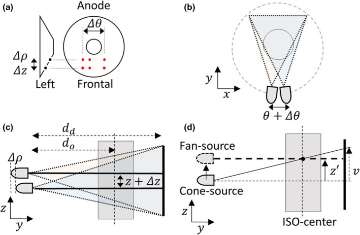
(a) Flying focal spots (6 red spots) at the anode plate and the shifts of (b) θ, (c) z and ρ directions by flying focal spot. (d) The determination of fanbeam line by the intersection of conebeam line and iso‐center, which is orthogonal to the z‐axis. Geometrically, Δz and Δρ move together.
4.B. Fast nonlocal weight calculation
In this paper, we developed the spatially encoded nonlocal penalty whose implementation is almost the same as the conventional nonlocal means. Note that the conventional nonlocal penalty is the same as the proposed method without the spatially encoded factor. One drawback of the proposed method is the high computational cost of patch difference for all patches. Based on the Darbon's method,26 we reduced the computational cost significantly using the accumulative summation approach, as shown in Fig. 3. For example, let's select two patches with center pixels of x i and x j within a neighbor window. The patch difference is the summation of individual pixel differences of two patches. Because two pixels of x i and x j are included in patch groups at the center and boundaries, the value of (x i −x j )2 should be calculated times if the difference value is computed patch‐by‐patch, which is the most time consuming process, particularly with large patch size . To calculate the difference between patches with a distance of (Δx,Δy) in Fig. 3(a), we first compute the difference of two images of I d (x,y) = (I(x,y)−I(x+Δx,y+Δy))2. Then, we calculate the accumulative summation image, , as shown in Fig. 3(b). The difference between the two patches can be computed using 4‐points, as shown in Fig. 3(c). Regardless of the patch size, we can calculate the difference using only 4‐points, and calculate the difference for all patches simultaneously. To extend to three‐dimension, the three‐dimensional accumulative summation and an 8‐point calculation are used.
Figure 3.
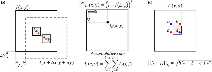
Fast nonlocal weight calculation in a two‐dimensional image. (a) Calculation of image difference with a distance of (Δx,Δy), (b) accumulative summation of the difference image, and (c) calculation of patch difference using 4‐points.
| Algorithm 2 Spatially encoded nonlocal penalty | |
|---|---|
| 1: Bind a 3D image to the texture memory. | |
| 2: Assign a specific voxel coordinate for each thread. | |
| 3: for do | |
| 4: Calculate the difference image I d = (I−I(Δ(x,y,z))2. | |
| 5: Calculate the accumulative summation image. | |
| 6: Calculate the weight using 8‐point execution. | |
| 7: Multiply the spatially encoded factor. | |
| 8: Calculate the weighted average value. | |
| 9: end for | |
| 10: Update the image |
| Algorithm 3 Forward and Backward Projectors | |
|---|---|
| Ray‐driven Projector | |
| 1: Bind a 3D image to the texture memory. | |
| 2: Assign a specific sinogram coordinate for each thread. | |
| 3: for each thread do | |
| 4: Calculate the coordinates of fan‐beam rays. | |
| 5: Add the interpolated voxel values along the ray. | |
| 6: Store the sum value. | |
| 7: end for | |
| Voxel‐driven Backprojector | |
| 1: Bind the sinogram to the texture memory. | |
| 2: State Assign a specific voxel coordinate for each thread. | |
| 3: for each thread do | |
| 4: Calculate all angular sinogram positions. | |
| 5: Add sinogram values and store the sum value. | |
| 6: end for |
4.C. Reconstruction
Recently, significant acceleration has been demonstrated for tomographic reconstruction using graphics processing units (GPUs).33, 34, 35, 36, 37 By extending previous works, we implemented the proposed method using GPU and CUDA. To efficiently use memory and threads in a GPU kernel, three main functions are separately parallelized: (a) spatially encoded nonlocal penalty, (b) forward projector, and (c) back‐projector.
In the implementation of spatially encoded nonlocal penalty, a GPU thread corresponds to a single voxel, and the texture memory binding with the image is used for the fast access, as described in algorithm 2. Because adjacent patches do not have a memory conflict or overlap, this implementation is efficient and feasible.18
In the iterative reconstruction, the most time consuming process is the image update, which contains forward projection and back‐projection operators. In our implementation, a ray‐driven projector and a voxel‐driven back‐projector are used in which a GPU thread corresponds to a ray and a voxel for forward projection and back‐projection, respectively. This kind of unmatched projectors have been widely used in the GPU‐based iterative reconstruction.33, 36, 37 Detailed steps of the ray‐driven projector and the voxel‐driven backprojector are summarized in algorithm 3.
5. Results
5.A. Dataset
For the validation of the proposed method, we used datasets supported by Low Dose CT Grand Challenge.24 In 10 training datasets, the regular dose projection data was acquired in Siemens Definition Flash scanner, and the quarter dose projection data was thoroughly synthesized. Datasets were acquired by raw projection measurements into Dicom format and the scatter counts were precorrected. In the geometry of scanner, the distance between source to isocenter is 595 mm and source to detector is 1085.6 mm. Δθ moves [−0.38∘,0.19∘,0.38∘], Δρ moves [0,5.45] mm and Δz moves [0,−0.66] mm, performing periodic motions on the anode plate. The detector size is 736 × 64 with a pixel resolution 1.2858 × 1.0947 mm. The ray from the central position hits the detector channel with 1.125 pixel shift from the center. All geometrical parameters were acquired from Dicom header using a special dictionary file. Single slice rebinning produced the 2‐D sinogram with size 736 × 2304 with 1 mm interval z‐slices. In most of the cases, spiral pitches were between 0.6 and 0.8. In the iterative reconstruction, an axial image interval of 1 mm was used. After reconstruction, we averaged the resulting image along z‐direction to create 3 mm wide images with 2 mm interval to satisfy Low Dose CT Grand Challenge submission criteria. The regular dose FBP image was used as ground‐truth. By comparing the regular dose FBP and the quarter dose data processed with the proposed method, the hyperparameters were estimated. Also, we compared the proposed method with l 1‐based 3‐D total variation (TV) penalty 38 and the conventional nonlocal penalty.
5.B. Hyperparameter selection
The hyperparameter selection is one of the most crucial factors for the image quality attainable with the proposed method. With the use of the regular dose image as ground truth, a bias and standard deviation study was conducted to find the best hyperparameters. For the bias and standard deviation study, we selected one dataset (L291) because the L291 dataset had more lesions. We first fixed the initial image, as a quarter dose FBP image using only the ramp filter, and 15 iterations (4 outer iterations starting with 8 subsets); because the FBP initial image is already close to solution, the small number of iterations was sufficient. Then, we could obtain the reconstructed image with a fixed number of iterations. In this paper, we empirically fixed τ = 0.01, κ = 3, Ω j = 9 × 9 × 9 and to reduce the number of hyperparameters. Because the β and σ were the most sensitive parameters to the image quality, the β and σ were estimated by comparing the bias and standard deviation between the regular dose FBP images and the processed quarter dose images. In Fig. 4, we compared the proposed method with l 1‐based total variation (TV) and the conventional nonlocal penalties. In our observation, the TV showed lower bias and the conventional nonlocal penalty showed lower standard deviation. However, we observed that both the bias and standard deviation of the proposed method showed better performance. Because the overall performance of TV was better than that of the conventional nonlocal method, we compared images with TV and the proposed method throughout the paper, and the best hyperparameters of Fig. 4(i) and (ii) were used for TV and proposed methods, respectively. The detailed bias and standard deviation values are listed in Table 1. All methods showed that the performance significantly varied by hyperparameters; therefore, the hyperparameter selection is the most important step in practice.
Figure 4.
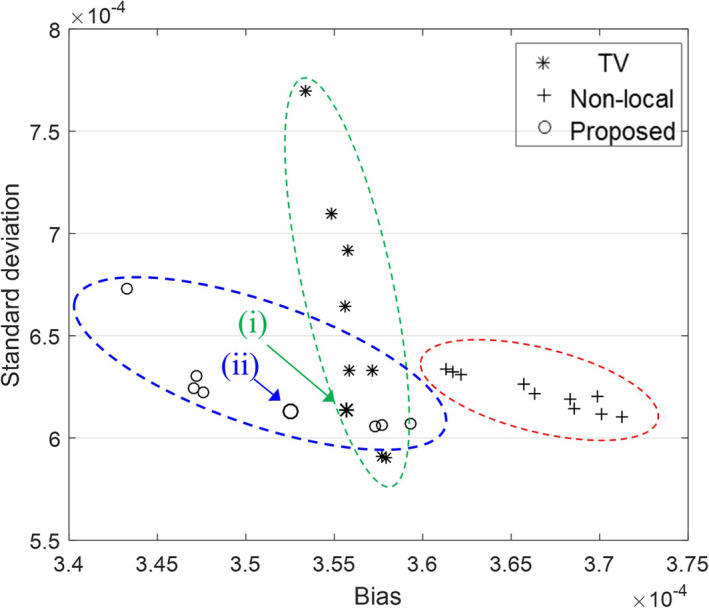
Bias and standard deviation plot for TV, the conventional nonlocal penalty, and the proposed method. The hyperparameters of (i) and (ii) were used for TV and the proposed method for the image comparison throughout our experiments.
Table 1.
Hyperparameter selection study for (a) TV and (b) proposed methods. STD denotes the standard deviation. The bias and standard deviation using the regular dose FBP image as ground truth and the processed quarter dose image were computed by various β, α and σ. Here, α is the soft‐thresholding value as used in the literature.16 The bold hyperparameters in (i) and (ii) were used for image quality comparison throughout our experiments, as shown in Fig. 4. Unit of bias and standard deviation is 10−4 mm−1
| (a) | β | α | Bias | STD |
|---|---|---|---|---|
| (i) | 0.02 | 0.0017 | 3.55 | 6.32 |
| 0.02 | 0.002 | 3.55 | 6.13 | |
| 0.03 | 0.0014 | 3.58 | 5.91 |
| (b) | β | σ | Bias | STD |
|---|---|---|---|---|
| (ii) | 0.01 | 0.037 | 3.47 | 6.22 |
| 0.02 | 0.037 | 3.52 | 6.12 | |
| 0.03 | 0.031 | 3.55 | 6.10 | |
| 0.04 | 0.031 | 3.57 | 6.00 |
5.C. Comparison of image quality
We first compared the reconstructed images using the accreditation (ACR) CT phantom as shown in Fig. 5. The reconstructed images using regular dose FBP, quarter dose FBP, TV, and the proposed method were compared. Because the noise level of ACR phantom data was much smaller than the noise level of patient datasets, the quarter dose FBP image still showed reliable quality. Using the hyperparameters of Fig. 4(i) and (ii), we also compared the reconstructed image using TV and the proposed method. Different high‐contrast resolution patterns from (i) to (iiii) in the same square (1.5 mm2) were compared. Window level was [−1000, 1300] HU and standard deviations in red circle were (a) 6.5, (b) 8.1, (c) 5.9 and (d) 6.1 HU in Fig. 5. With similar background noise levels, the contrast of the proposed method is visually clearer than the contrast of TV. We confirmed that the proposed method can reduce the noise while preserving the high‐contrast regions.
Figure 5.
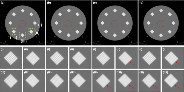
The reconstructed images of the ACR phantom using (a) regular dose FBP, (b) quarter dose FBP, (c) TV and (d) the proposed method. High‐contrast resolution patterns from (i) to (iiii) in the same square (1.5 mm2) were compared. Window level was [‐1000, 1300] HU and standard deviations in red circle were (a) 6.5, (b) 8.1, (c) 5.9, and (d) 6.1 HU.
We compared the reconstructed images of three patients with metastatic lesions in Figs. 6, 7, 8. The reconstructed images using regular dose FBP, quarter dose FBP, quarter dose TV, and quarter dose proposed method were compared. Here, the ramp filter was applied in the quarter dose FBP to show the degradation of image quality. Intensity range was 40 ± 200 HU and metastatic lesions are pointed by arrows as shown in Figs. 6, 7, 8. The reconstructed images using TV contained both blurred and still noisy regions compared to the images using the proposed method. The results demonstrated that the proposed method significantly reduced noise while preserving contrast and diagnostic features.
Figure 6.
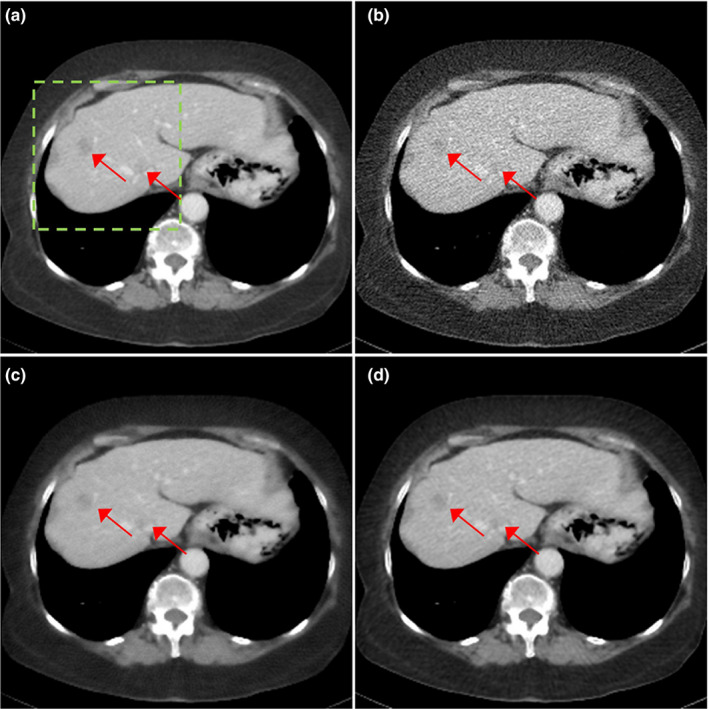
Patient of L096 with metastatic lesions. The reconstructed images using (a) regular dose FBP, (b) quarter dose FBP, (c) quarter dose TV, and (d) quarter dose proposed method were compared. Intensity range is 40 ± 200 HU. Metastatic lesions are pointed by red arrows.
Figure 7.
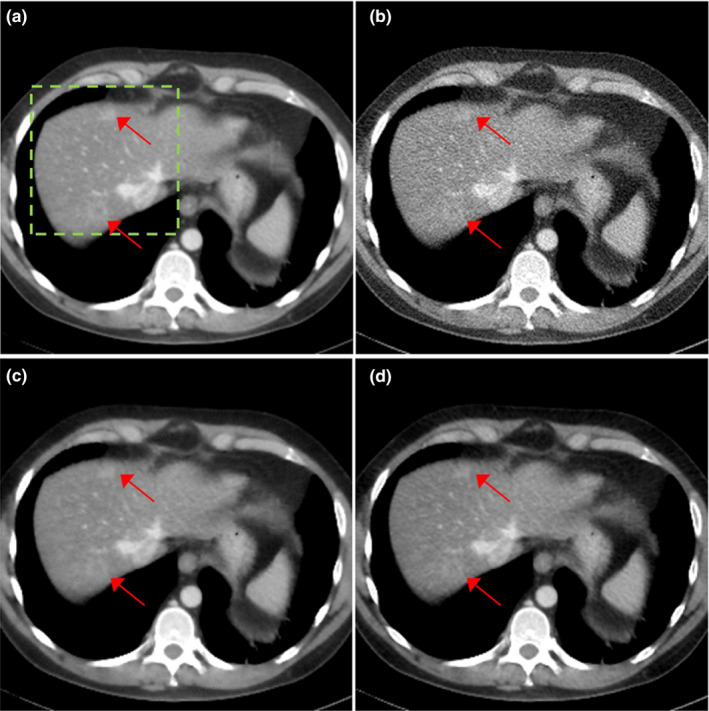
Patient of L291 with metastatic lesions. The reconstructed images using (a) regular dose FBP, (b) quarter dose FBP, (c) quarter dose TV and (d) quarter dose proposed method were compared. Intensity range is 40 ± 200 HU. Metastatic lesions are pointed by red arrows.
Figure 8.
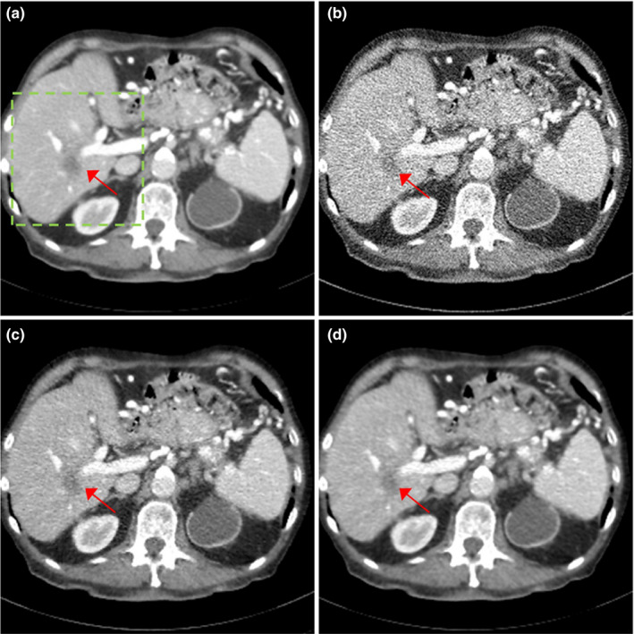
Patient of L506 with metastatic lesions. The reconstructed images using (a) regular dose FBP, (b) quarter dose FBP, (c) quarter dose TV, and (d) quarter dose proposed method were compared. Intensity range is 40 ± 200 HU. Metastatic lesions are pointed by red arrows.
In addition, the reconstructed images of TV and proposed methods using patient data (L143) were compared with the axial, coronal and saggital views as shown in Fig. 9, and the same hyperparameters of Fig. 4(i) and (ii) were used. Intensity range was 40 ± 200 HU and yellow circle indicated a metastatic lesion. Metastatic lesions of TV and the proposed method in axial views were both recognizable with slightly different contrasts. However, in coronal views, some parts of the reconstructed images using TV were still noisier than the image using the proposed method (see arrows in Fig. 9). In the Low Dose CT Grand Challenge, we submitted reconstructed images for test datasets of 20 patients using the same hyperparameters, and the image quality was evaluated by radiologists at the Mayo clinic.
Figure 9.
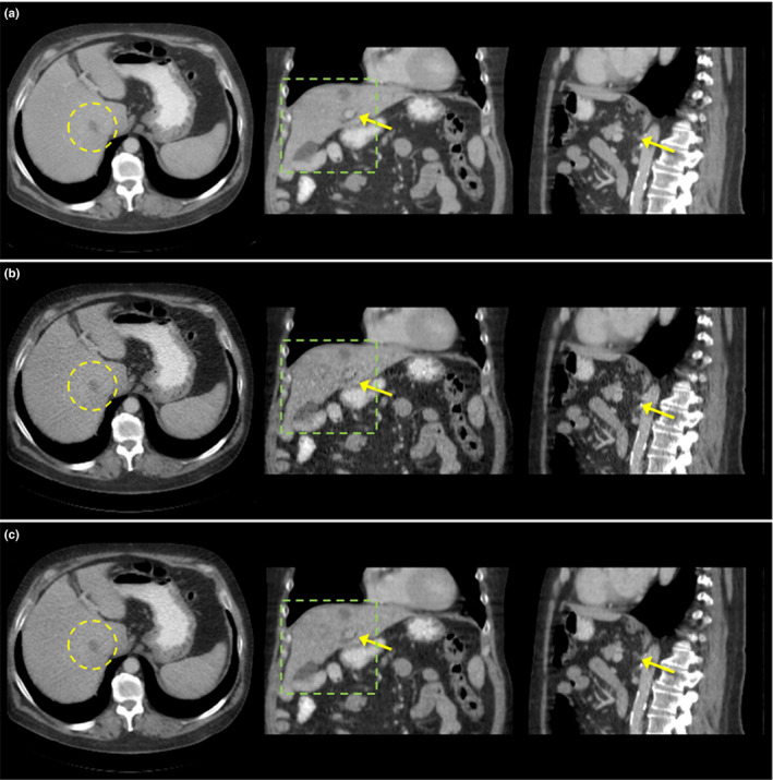
Comparison of reconstructed images of patient (L143) using (a) regular dose FBP, (b) quarter dose TV, and (c) quarter dose proposed method. Axial, coronal, and saggital views were compared. Intensity range is 40 ± 200 HU. Yellow circle indicates the metastatic lesion.
We applied the Nesterov's momentum and the diminishing number of subsets for further improvement. For the validation, we calculated the mean square errors of the reconstructed images using the proposed method (a) without diminishing subsets and momentum, (b) with diminishing subsets and without momentum, and (c) with diminishing subsets and momentum as shown in Fig. 10. The effect of the diminishing number of subsets was small, however, the proposed method using the momentum method converged faster, which can be useful when we fix the small number of iterations, as was done in this paper. Note that our results were not converged image due to the fixed number of iterations and the momentum. Thus, to obtain best images, the proposed method can have many solutions affected by not only hyperparameters but also initial settings such as initial image and the numbers of subsets and iterations.
Figure 10.
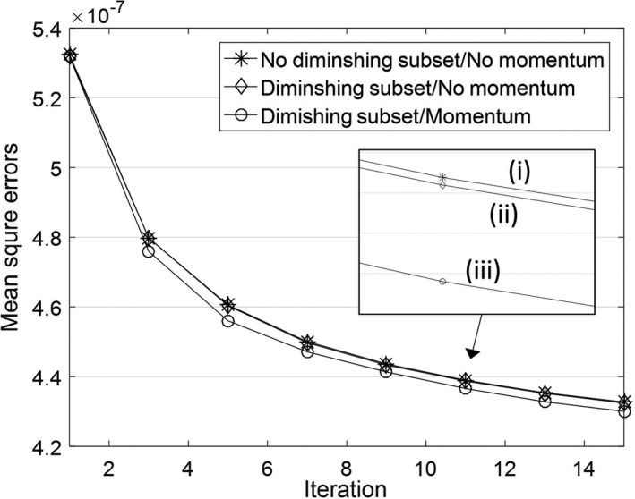
Mean square errors of the reconstructed images using the proposed method (i) without diminishing subsets and momentum, (ii) with diminishing subsets and without momentum, and (iii) with diminishing subsets and momentum.
5.D. Execution time
We used Nvidia's Titan GPU and CUDA in Matlab. Main functions, such as forward, backward projectors, and the spatially encoded nonlocal penalty, were implemented in Mex function of Matlab with CUDA. In geometry of the sinogram with 736 × 2203 × 128 (radial, azimuthal, and axial) and the image 512 × 512 × 128 (x,y,z), the projection, back‐projection, and penalty functions took less than 5, 3, and 11 s, respectively, which are more than 100 times faster than CPU‐based implementations. Execution time is proportional to the number of slices and the number of iterations. As we mentioned before, slice rebinning with 1 mm was used for reconstruction, and the axial 3 mm average with 2 mm interval was applied for the submission. In test datasets, the number of average slices rebinning with 1 mm were 210 and 15 iterations were used, which took about total 8 min.
6. Discussion
Theoretically, a true in is crucial to guarantee the convergence. Practically, we replaced by x (n−1) in iteration, which leads to a varying cost function and a nonguaranteed convergence. Intuitively, if the sequence of x (n−1) can converge to in iteration under certain conditions, then the optimization can eventually converge. However, there is no guarantee that the converging point is independent of the initial condition. Thus, in our algorithm, an initial image close to the optimal solution is important. In this paper, we set the initial image as quarter dose FBP image. In addition, we compared the image quality of two alternatives of discussed in Section 3.B, as demonstrated in Fig. 11. The reconstructed image using quarter dose FBP image as fixed in Fig. 11(a) was noisy, which could potentially lead to misdiagnosis. We confirmed that the reconstructed image using the x (n−1) as in Fig. 11(b) was considerably less noisy.
Figure 11.
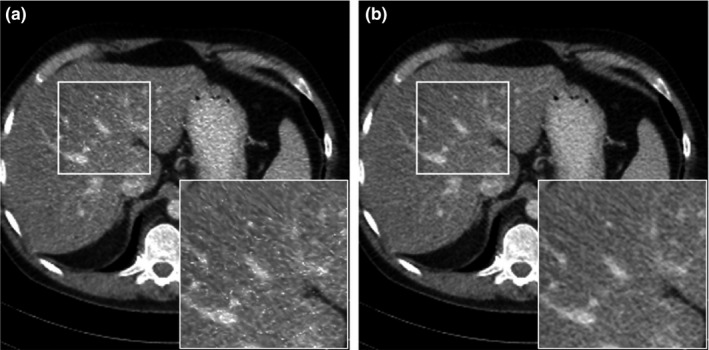
Comparison of reconstructed images using (a) fixed as quarter dose FBP image and using (b) as x (n−1). n denotes the iteration number.
Although we have reduced the noise significantly, we still need to improve the image quality for diagnosis. In Fig. 12, we showed several unclear lesions of metastasis, such as focal fat/ focal fatty sparing and perfusion defect. We observed lesions very carefully with changing hyperparameters, however, we could not clearly identify some lesions using the proposed method. Also, the number of datasets in this paper was limited, thus, further evaluation is required with sufficient number of datasets.
Figure 12.
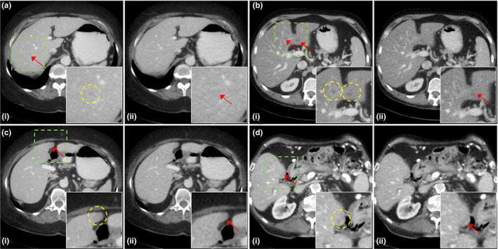
Unclear lesions of (a) metastasis (L096), (b) focal fat/ focal fatty sparing (L291), (c) perfusion defect (L096), and (d) metastasis (L506). The reconstructed images using (i) regular dose FBP and (ii) quarter dose proposed method were compared. Yellow circles in (i) showed the lesions. Intensity range is 40 ± 200 HU.
In Fig. 13, we introduce one patient (L096) who has a pacemaker in the heart region. We observed the streaking artifacts due to the metal object containing the main device and wires. We compared FBP images of regular dose and quarter dose, and the reconstructed image using the proposed method. Although the proposed method can remove noise significantly, streaking artifacts were not removed in our iterative reconstruction. In our future works, it is required to develop a new method not only providing clearer lesion features but also correcting beam‐hardening and metal artifacts for further image improvement using clinical lower dose data.
Figure 13.
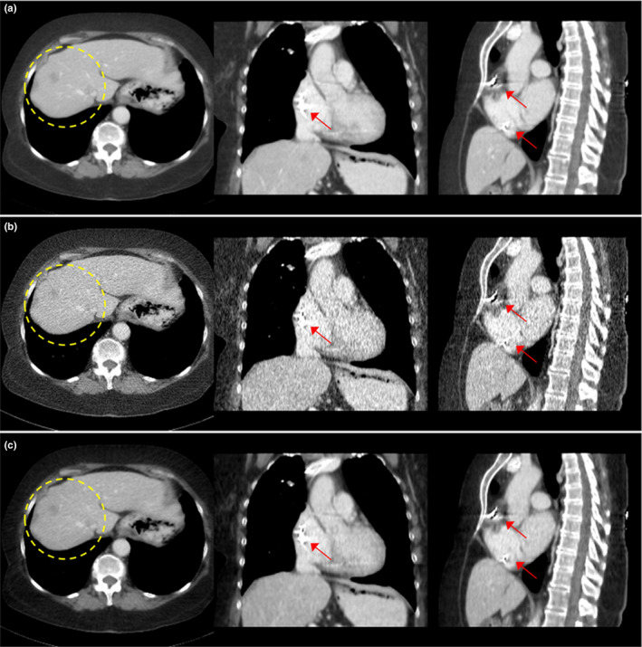
Comparison of reconstructed images of patient data (L096) using (a) regular dose FBP, (b) quarter dose FBP, and (c) quarter dose proposed method. The circle in axial view indicates metastasis lesions and arrows indicate the metallic object (pacemaker). Intensity range is 40 ± 200 HU.
7. Conclusion
In this paper, we proposed an empirical iterative CT reconstruction method using spatially encoded nonlocal penalty and ordered subsets separable quadratic surrogates (OS‐SQS) with Nesterov's momentum and diminishing number of subsets. We selected the best hyperparameters by conducting a bias and standard deviation study using regular dose image as ground truth. We compared the reconstructed images using regular dose FBP, quarter dose FBP, quarter dose 3‐D TV, and quarter dose proposed method. The results of ACR CT phantom and patient datasets demonstrated that the proposed method with fine‐tuned hyperparameters significantly improved the image quality at quarter dose. Furthermore, the single slice rebinning using 64 multislice detector with flying focal spot was used for the computational efficiency and GPU implementation significantly reduced execution time, which make the proposed method clinically practical. The performance of the proposed method should be further improved for small lesions, and more thorough evaluation using sufficient clinical data is required in the future work.
Conflict of interest
The authors declare that they do not have any conflict of interest.
Supporting information
Appendix S1
Appendix S2
Acknowledgment
We would like to specially thank associate editor for editorial comments which improved the manuscript of better quality.
References
- 1. Hsieh J. Computed Tomography: Principles, Design, Artifacts, and Recent Advances. Bellingham, WA: SPIE; 2003. [Google Scholar]
- 2. Hara AK, Paden RG, Silva AC, Kujak JL, Lawder HJ, Pavlicek W. Iterative reconstruction technique for reducing body radiation dose at CT: feasibility study. Am J Roentgenol. 2009;193:764–771. [DOI] [PubMed] [Google Scholar]
- 3. Thibault J‐B, Sauer KD, Bouman CA, Hsieh J. A three‐dimensional statistical approach to improved image quality for multislice helical CT. Med Phys. 2007;34:4526–4544. [DOI] [PubMed] [Google Scholar]
- 4. Shepp LA, Vardi Y. Maximum likelihood reconstruction for emission tomography. IEEE Trans Med Imag. 1982;1:113–122. [DOI] [PubMed] [Google Scholar]
- 5. Hudson HM, Larkin RS. Accelerated image reconstruction using ordered subsets of projection data. IEEE Trans Med Imag. 1994;13:601–609. [DOI] [PubMed] [Google Scholar]
- 6. Gordon R, Bender R, Herman GT. Algebraic reconstruction techniques (ART) for three‐dimensional electron microscopy and X‐ray photography. J Theoretical Biol. 1970;29:471–481. [DOI] [PubMed] [Google Scholar]
- 7. Andersen AH, Kak AC. Simultaneous algebraic reconstruction technique (SART): a superior implementation of the ART algorithm. Ultrason Imaging. 1984;6:81–94. [DOI] [PubMed] [Google Scholar]
- 8. Erdogan H, Fessler JA. Ordered subsets algorithms for transmission tomography. Phys Med Biol. 1999;44:2835–2851. [DOI] [PubMed] [Google Scholar]
- 9. Lindenbaum M, Fischer M, Bruckstein A. On Gabor's contribution to image enhancement. Pattern Recognit. 1994;27:1–8. [Google Scholar]
- 10. Charbonnier P, Blanc‐Féraud L, Aubert G, Bar‐laud M. Deterministic edge‐preserving regularization in computed imaging. IEEE Trans Image Process. 1997;6:298–311. [DOI] [PubMed] [Google Scholar]
- 11. Rudin LI, Osher S. Total variation based image restoration with free local constraints. In: International Conference on Image Processing. Vol. 1. IEEE; 1994:31–35. [Google Scholar]
- 12. Buades A, Coll B, Morel J‐M. A non‐local algorithm for image denoising. In: Computer Society Conference on Computer Vision and Pattern Recognition. Vol. 2. IEEE; 2005:60–65. [Google Scholar]
- 13. Chang SG, Yu B, Vetterli M. Adaptive wavelet thresholding for image denoising and compression. IEEE Trans Image Process. 2000;9:1532–1546. [DOI] [PubMed] [Google Scholar]
- 14. Chambolle A. An algorithm for total variation minimization and applications. J Math Imaging Vis. 2004;20:89–97. [Google Scholar]
- 15. Sidky EY, Pan X. Image reconstruction in circular cone‐beam computed tomography by constrained, total‐variation minimization. Phys Med Biol. 2008;53:4777–4807. [DOI] [PMC free article] [PubMed] [Google Scholar]
- 16. Yin W, Osher S, Goldfarb D, Darbon J. Bregman iterative algorithms for l1‐minimization with applications to compressed sensing. SIAM J Imaging Sci. 2008;1:143–168. [Google Scholar]
- 17. Dabov K, Foi A, Katkovnik V, Egiazarian K. Image denoising by sparse 3‐D transform‐domain collaborative filtering. IEEE Trans Image Process. 2007;16:2080–2095. [DOI] [PubMed] [Google Scholar]
- 18. Kim K, Ye JC, Worstell W, et al. Sparse‐view spectral CT reconstruction using spectral patch‐based low‐rank penalty. IEEE Trans Med Imaging. 2015;34:748–760. [DOI] [PubMed] [Google Scholar]
- 19. Wang G, Qi J. Penalized likelihood PET image reconstruction using patch‐based edge‐preserving regularization. IEEE Trans Med Imaging. 2012;31:2194–2204. [DOI] [PMC free article] [PubMed] [Google Scholar]
- 20. Yang Z, Jacob M. Nonlocal regularization of inverse problems: a unified variational framework. IEEE Trans Image Process. 2013;22:3192–3203. [DOI] [PMC free article] [PubMed] [Google Scholar]
- 21. Nuyts J, Beque D, Dupont P, Mortelmans L. A concave prior penalizing relative differences for maximum‐a‐posteriori reconstruction in emission tomography. IEEE Trans Nucl Sci. 2002:49:56–60. [Google Scholar]
- 22. Qi J, Leahy RM. Resolution and noise properties of MAP reconstruction for fully 3‐D PET. IEEE Trans Med Imaging. 2000;19:493–506. [DOI] [PubMed] [Google Scholar]
- 23. Li Q, Bai B, Cho S, Smith A, Leahy R. Count independent resolution and its calibration. In: International Meeting on Fully Three‐Dimensional Image Reconstruction in Radiology and Nuclear Medicine. IEEE; 2009:223–226. [Google Scholar]
- 24. McCollough C. TU‐FG‐207A‐04: overview of the low dose CT grand challenge. (http://www.aapm.org/GrandChallenge/LowDoseCT/). Med Phys. 2016;43:3759–3760. [Google Scholar]
- 25. Devolder O, Glineur F, Nesterov Y. First‐order methods of smooth convex optimization with inexact oracle. Math Program. 2014;146:37–75. [Google Scholar]
- 26. Darbon J, Cunha A, Chan TF, Osher S, Jensen GJ. Fast nonlocal filtering applied to electron cryomicroscopy. In: IEEE International Symposium on Biomedical Imaging. IEEE; 2008:1331–1334. [Google Scholar]
- 27. Noo F, Defrise M, Clackdoyle R. Single‐slice rebinning method for helical cone‐beam CT. Phys Med Biol. 1999;44:561–570. [DOI] [PubMed] [Google Scholar]
- 28. Flohr T, Stierstorfer K, Ulzheimer S, Bruder H, Primak A, McCollough CH, Image reconstruction and image quality evaluation for a 64‐slice CT scanner with z‐ying focal spot. Med Phys. 2005;32:2536–2547. [DOI] [PubMed] [Google Scholar]
- 29. Dabov K, Foi A, Katkovnik V, Egiazarian K. Image denoising with block‐matching and 3D filtering. SPIE. 2006;6064:606414. [Google Scholar]
- 30. Gilboa G, Osher S. Nonlocal linear image regularization and supervised segmentation. Multiscale Model Simul. 2007;6:595–630. [Google Scholar]
- 31. Elmoataz A, Lezoray O, Bougleux S. Nonlocal discrete regularization on weighted graphs: a framework for image and manifold processing. IEEE Trans Image Process. 2008;17:1047–1060. [DOI] [PubMed] [Google Scholar]
- 32. Kim D, Ramani S, Fessler JA. Combining ordered subsets and momentum for accelerated X‐ray CT image reconstruction. IEEE Trans Med Imaging. 2015;34:167–178. [DOI] [PMC free article] [PubMed] [Google Scholar]
- 33. Kim K, Ye JC. Fully 3D iterative scatter‐corrected OSEM for HRRT PET using a GPU. Phys Med Biol. 2011;56:4991–5009. [DOI] [PubMed] [Google Scholar]
- 34. Mueller K,Xu F. Practical considerations for GPU‐accelerated CT. In: International Symposium on Biomedical Imaging. IEEE; 2006:1184–1187. [Google Scholar]
- 35. Sharp G, Kandasamy N, Singh H, Folkert M. GPU‐based streaming architectures for fast cone‐beam CT image reconstruction and demons deformable registration. Phys Med Biol. 2007;52:5771–5783. [DOI] [PubMed] [Google Scholar]
- 36. Yan G, Tian J, Zhu S, Dai Y, Qin C. Fast cone‐beam CT image reconstruction using GPU hardware. J Xray Sci Technol. 2008;16:225–234. [Google Scholar]
- 37. Jia X, Lou Y, Li R, Song WY, Jiang SB. GPU‐ based fast cone beam CT reconstruction from undersampled and noisy projection data via total variation. Med Phys. 2010;37:1760. [DOI] [PubMed] [Google Scholar]
- 38. Kim K, Dutta J, Groll A, Fakhri GE, Meng L‐J, Li Q. Penalized maximum likelihood reconstruction of ultra‐high resolution PET with depth of interaction. In: International Meeting on Fully Three‐Dimensional Image Reconstruction in Radiology and Nuclear Medicine. IEEE; 2015:296–299. [Google Scholar]
Associated Data
This section collects any data citations, data availability statements, or supplementary materials included in this article.
Supplementary Materials
Appendix S1
Appendix S2


