Whole-Volume Clustering of Time Series Data from Zebrafish Brain Calcium Images via Mixture Modeling

Abstract

Calcium is a ubiquitous messenger in neural signaling events. An increasing number of techniques are enabling visualization of neurological activity in animal models via luminescent proteins that bind to calcium ions. These techniques generate large volumes of spatially correlated time series. A model-based functional data analysis methodology via Gaussian mixtures is suggested for the clustering of data from such visualizations is proposed. The methodology is theoretically justified and a computationally efficient approach to estimation is suggested. An example analysis of a zebrafish imaging experiment is presented.

1 Introduction

Calcium is a ubiquitous secondary messenger that regulates vital signaling events in neurons and other excitable cells [1]. In neurons, synaptic input and action potential firing trigger the rapid input of large quantities of calcium ions [2]. By fusing a calcium-binding domain to a fluorescent protein it is possible to monitor calcium ions and therefore various spike features [3]. Genetically encoded calcium indicators (GECIs) can target specific cell types or subcellular compartments and have facilitated long-term optical recording of genetically targeted neurons in vivo. GECIs like GCaMP are the most widely used calcium indicators [4] and a range of mouse, drosophila, and zebrafish lines have been generated that express GCaMP pan-neuronally.

In recent years, the zebrafish has become a popular model in neurological research (e.g. [5] and [6]) and the number of studies imaging neuronal calcium dynamics in larval zebrafish has increased dramatically (e.g. [7] and [8]). Larval zebrafish are particularly amenable to calcium imaging as they are translucent making it easy to image large populations of neurons without surgery, possess a relatively small brain (≈ 800 × 600 × 200 μm³) thereby facilitating whole-brain imaging [9], and the generation of transgenic lines is relatively straightforward promoting the creation of a range of transgenic lines [10]. Light-sheet based microscopy methods can enable imaging in larval zebrafish with sufficient temporal resolution to record neural dynamics throughout the brain [5].

In this article, we devise a method for clustering time series that are obtained from whole-volume calcium imaging experiments. Large time series data sets, consisting of thousands of time points, were acquired using using swept confocally-aligned planar excitation microscopy (SCAPE; [11]). SCAPE is a novel method for high-speed light sheet imaging, which enables imaging of the entire zebrafish brain using a single objective lens in a flexible geometry and at very high spatiotemporal resolution. The data set utilized here was a whole-volume calcium image of a larval zebrafish brain at a spatial resolution of 640 × 130 × 300 (x × y × z) voxels and a temporal resolution of 4 volumes per second.

Two primary factors make the clustering of whole-volume calcium imaging time series difficult. Firstly, the time series can often be obtained at sparse or irregular intervals. Secondly, the size of the data firmly places the problem within the realms of Big Data, where conventional methods are infeasible to implement (cf. [12, Sec. 1.2]). The method that we develop in this article is designed to address these primary concerns.

Time series clustering is a well-studied area in data analysis and signals processing; see [13] and [14] for recent literature reviews. From [14], it is clear that there are numerous approaches to the problem of time series clustering. Due to the high dimensionality of the raw time series that arise from calcium imaging experiments, an abstraction is necessary to limit computational burden. The general framework of functional data analysis (FDA) is amenable to our aims; see [15] for an introduction to FDA. In this article, we present a mixture model-based functional data approach, thus only a brief literature review of such methods will be provided in the sequel.

In [16], a mixture of polynomial basis-filtered models was suggested for the clustering of time-dependent trajectories. In [17], a regularized mixture of mixed-effects (MEM) basis-filtered models using B-splines was considered for the clustering of sparsely-sampled univariate functional data. Both [18] and [19] suggested MEM basis-filtered models using Fourier bases for clustering of time-course gene expression data; [20] extended the method of [19] by allowing for autoregressive (AR) errors. An extension of the MEM model of [19] that allowed for concomitant covariates was proposed in [21]. An adaptation of the MEM model from [17] was suggested for the clustering of sparsely-sampled bivariate functional data in [22]. Lastly, a set of methods that are related to the mixture model-based FDA approach are the mixtures of AR models that utilize a parametric stochastic process abstraction of the time series instead; see [23], [24], and [25].

In this article, we consider a two-stage approach to clustering the calcium image obtained time series that is adapted from that of [26]. In the first stage, each time series is filtered via a common set of B-spline bases using ordinary least squares (OLS); this produces a set of basis coefficients for each time series. Here, our notion of filtering as an operation that projects the time series into a lower-dimensional space is the same as that of [17]. In the second stage, a GMM-like (Gaussian mixture model; for example, see [27, Ch. 3]) clustering of the basis coefficients for each time series is conducted to partition the time series into k classes, where k is determined by a BIC-like (Bayesian information criterion [28]) approach via the slope heuristic technique of [29]. In this article, we use the trimmed k-means algorithm [30] for clustering due to its speed in the large data context. The two-stage nature of our method shares similarities with the methods of [31] and [32].

To justify our two-stage approach, we demonstrate that it permits the same statistical interpretation as the MEM model of [17]. Although the method of [17] permits sparseness and irregularity in the time series, the iterative and slow-converging EM (expectation–maximization [33]) algorithm that is required for its implementation is inappropriate for data sizes in calcium imaging time series clustering; the same reasoning applies to the infeasibility of the MEM model-based methods; see [26, Sec. 4] for details. The methods that are based on mixtures of AR models are also inappropriate in this context due to their inability to handle sparsity in the sampling of the time series.

Along with the statistical model for calcium imaging, time series clustering, and two-stage method for performing the clustering, we also discuss the theoretical conditions under which the maximum likelihood (ML) estimator of a GMM model is consistent, under dependence between spatially correlated voxels. We then extend this discussion towards the suitability of the trimmed k-means algorithm. A numerical study is provided to justify our approach. To demonstrate an application of our methodology, we conduct a clustering of time series data arising from a whole-volume calcium imaging experiment of a larval zebrafish brain at rest, acquired using SCAPE microscopy.

The rest of the article proceeds as follows. A statistical model for calcium imaging time series clustering is presented in Section 2. A two-stage algorithm is suggested for performing clustering in Section 3. An application to a zebrafish brain calcium imaging data is presented in Section 4. Conclusions are drawn in Section 5. A description of the trimmed k-means method is also provided in the Appendix.

2 Statistical Model

Suppose that we wish to cluster a sample of time series ${\mathcal{Y}}_n=\{Y_1(t),\dots ,Y_n(t)\}$ that are treated as functions in t on some interval $\mathbb{T}$. Let each time series Y_i (t) (i = 1, …, n) be observed at m_i time points t₁, …, $t_{m_i}\in \mathbb{T}$ (they may be sparsely and irregularly sampled) and suppose that we observe Y_i at t_j (j = 1, …, m_i) indirectly via the noise-corrupted variable

$$Z_i(t_j)=Y_i(t_j)+E_i(t_j),$$ (1)

where E_i (t_j) is a random error from a univariate Gaussian density distribution with mean 0 and variance σ².

In order to cluster the data, we require an implicit model for the subpopulation heterogeneity of the elements in ${\mathcal{Y}}_n$. We propose a parametric model for the purpose. Let $Y_i(t)={\mathit{B}}_i^T\mathit{x}(t)$, where x (t) is a d-dimensional vector of evaluates at point t of a B-spline system with (d − 2)-breakpoints over $\mathbb{T}$ (see [34, Ch. 9]), and let B_i ∈ ℝ^d be a random variable that captures the heterogeneity of ${\mathcal{Y}}_n$. Here, the superscript T indicates matrix transposition. Cubic B-splines are used in all of our applications. We suppose that the B-spline representation B_i arises from a k-component GMM with density function

$$f(\mathit{b};\mathit{\theta })={\displaystyle \sum _{c=1}^k{\pi }_c{\varphi }_d(\mathit{b};{\mathit{\mu }}_c,{\mathbf{V}}_c)},$$ (2)

where π_c > 0, ${\displaystyle {\sum }_{c=1}^k{\pi }_c=1}$, μ_c ∈ ℝ^d, V_c ∈ ℝ^d×d is positive definite (c = 1, …, k), and

$${\varphi }_d(\mathit{b};\mathit{\mu },\mathbf{V})=|2\pi \mathbf{V}{|}^{-1/2}\exp \left[-\frac{1}{2}{(\mathit{b}-\mathit{\mu })}^T{\mathbf{V}}^{-1}(\mathit{b}-\mathit{\mu })\right]$$

is the multivariate Gaussian density function with mean μ and covariance matrix V. We shall refer to π_c as the prior probability of observing Y_i is in cluster c, and ϕ_d (b; μ, V) as the component density function of cluster c. Here, we put the parameter components π_c, μ_c, and V_c into the vector θ.

Remark 1

Any linear basis system can be used in place of the B-splines in this article. Examples of other basis systems are Fourier or polynomial bases; see [15, Sec. 3.3].

The model described so far is close to that of [17]. However, in order to proceed as [17] does, estimation of each B_i is required using the data Z_i (t_j), for all i and j, via an EM algorithm. This is not feasible in the setting that we wish to conduct clustering. We instead suggest that we estimate each B_i only via the data Z_i (t_j) for the same i. We do this via the OLS estimator

$${\stackrel{\sim }{\mathit{B}}}_i={({\mathbf{X}}_i^T{\mathbf{X}}_i)}^{-1}{\mathbf{X}}_i^T{\mathit{Z}}_i,$$ (3)

where we let ${\mathbf{X}}_i^T=\left[\mathit{x}(t_1)\cdots \mathit{x}(t_{m_i})\right]$ and ${\mathit{Z}}_i^T=(Z_i(t_1),\dots ,Z_i(t_{m_i}))$. The following result is proved in [26].

Proposition 1

Under characterizations (1) and (2), ${\stackrel{\sim }{\mathit{B}}}_i$ (as characterized by (3)) has density function

$$f\left({\stackrel{\sim }{\mathit{b}}}_i;\vartheta \right)={\displaystyle \sum _{c=1}^k{\pi }_c{\varphi }_d}\left({\stackrel{\sim }{\mathit{b}}}_i;{\mathit{\mu }}_c,{\mathbf{V}}_c+{\sigma }^2{\left[{\mathbf{X}}_i^T{\mathbf{X}}_i\right]}^{-1}\right),$$ (4)

where we put the parameter components π_c, μ_c, V_c, and σ² into ϑ.

Remark 2

Density (4) is dependent on i only via the term ${\sigma }^2{\left[{\mathbf{X}}_i^T{\mathbf{X}}_i\right]}^{-1}$. If we let X_i = X for all i, then we can write

$$f\left(\stackrel{\sim }{\mathit{b}},\psi \right)={\displaystyle \sum _{c=1}^k{\pi }_c{\varphi }_d}\left(\stackrel{\sim }{\mathit{b}};{\mathit{\mu }}_c,{\stackrel{\sim }{\mathbf{V}}}_c\right),$$ (5)

where ${\stackrel{\sim }{\mathbf{V}}}_c={\mathbf{V}}_c+{\sigma }^2{[{\mathbf{X}}^T\mathbf{X}]}^{-1}$ and ψ contains the parameter components of the model.

Remark 3

Alternatively to Remark 2, if we assume some structure in the sampling of the time points t₁, …, $t_{m_i}$ for each i, then we can reasonably assume that ${\mathbf{X}}_i^T{\mathbf{X}}_i$ approaches some positive and invertible matrix Δ in probability, for each i, as n approaches infinity. In such a case, an appropriate Slutsky-type theorem would imply that ${\stackrel{\sim }{\mathit{B}}}_i$ approaches a random variable with a mixture distribution of form (4), where ${\mathbf{X}}_i^T{\mathbf{X}}_i$ is replaced by Δ.

Remark 4

It is possible that for some choice of m_i and d, the matrix product ${\mathbf{X}}_i^T{\mathbf{X}}_i$ may be singular. In such situations, we may replace ${\left({\mathbf{X}}_i^T{\mathbf{X}}_i\right)}^{-1}$ is (3)–(5) by the Moore-Penrose inverse ${\left({\mathbf{X}}_i^T{\mathbf{X}}_i\right)}^{+}$, instead. Since the Moore-Penrose inverse is unique and always exists, its use in our application causes no unintended effects (cf. [35, Sec. 7.4]).

2.1 Parameter Estimation

Suppose that we observe data z_i that are realizations of Z_i from the process (1). Also suppose that $\{t_1,\dots t_{m_i}\}=\{t_1,\dots t_m\}$ for all i (i.e. X_i = X for all i, from Remark 2). A natural parameter estimator for ψ in (5) is the MLE (maximum likelihood estimator). Define ∇ as the gradient operator, and let the MLE be ${\widehat{\mathit{\psi }}}_n$, which is a suitable root of ${\mathcal{l}}_n(\mathit{\psi })={\displaystyle {\sum }_{i=1}^n\log f\left({\stackrel{\sim }{\mathit{b}}}_i;\mathit{\psi }\right)}$, where ${\stackrel{\sim }{\mathit{b}}}_i={\left({\mathbf{X}}^T\mathbf{X}\right)}^{-1}{\mathbf{X}}^T{\mathit{z}}_i$. The following useful result regarding the consistency of MLE under dependence (e.g. spatial dependence between voxels in imaging data) is obtained in [26].

Proposition 2

Let Z₁, …, Z_n be an identically distributed (ID) and stationary ergodic (or strong-mixing) random sample (as characterized by (1)), which generates a set of OLS estimators ${\stackrel{\sim }{\mathit{B}}}_1$, …, ${\stackrel{\sim }{\mathit{B}}}_n$. Suppose that each ${\stackrel{\sim }{\mathit{B}}}_i(i=1,\dots ,n)$ arises from a distribution with density $f\left(\stackrel{\sim }{\mathit{b}},{\mathit{\psi }}_0\right)$, where ψ₀ (containing π_0c, μ_0c, and V_0c for all c) is a strict-local maximizer of $\mathbb{E}$ log $f\left(\stackrel{\sim }{\mathit{b}};\mathit{\psi }\right)$. If Ψ_n = {ψ : ∇ℓ_n = 0} (where we take ${\Psi }_n=\left\{\overline{\mathit{\psi }}\right\}$, for some $\overline{\mathit{\psi }}$ in the domain of $f\left(\stackrel{\sim }{\mathit{b}};\mathit{\psi }\right)$, if ∇ℓ_n = 0 has no solution), then for any ε > 0,

$$\underset{n\to \infty }{\lim }\mathbb{P}\left[\underset{\mathit{\psi }\to {\Psi }_n}{\inf }{(\mathit{\psi }-{\mathit{\psi }}_0)}^T(\mathit{\psi }-{\mathit{\psi }}_0)>\epsilon \right]=0.$$

The result establishes the fact that there exists a consistent root to the like-lihood score equation ∇ℓ_n = 0. This is a useful result since the likelihood for a GMM cannot possess a unique global maximum as it is unbounded and lacks identifiability. The proof of Proposition 2 invokes an extremum estimator theorem [36, Thm. 4.1.2] in conjunction with either an ergodic continuous mapping theorem or a strong-mixing continuous mapping theorem (see [37, Thms. 3.35 and 3.49]). A generic uniform law of large numbers (ULLN) such as [38, Thm. 5] can then be used to obtain the desired result; see [24, Appendix I] for the proof of a similar result.

Remark 5

Strong mixing can be guaranteed by assuming that the sequence Z_i is M-dependent (cf. [39, Sec. 2.1]). That is, there exists some M < ∞ such that if |i − i′| > M then Z_i and Z_i′ are independent. This is a reasonable assumption in imaging applications where features behave in locally coherent groups.

Remark 6

The intended use of this article is for clustering time series at voxels on a three-dimensional array. The asymptotics of Proposition 2 in conjunction with Remark 5 applies when one of the three dimensions are extended infinitely. In practice, this is unimportant, but a theoretical labelling of the voxels that would allow the M-dependent assumption to hold when all three dimensions are extended would be difficult. One could instead treat the problem as an estimation problem over data arising from a stationary three-dimensional mixing random field. In such a case, the M-dependent assumption of Remark 5 can still be made (cf. [40]). The generic ULLN of [41] can be used in place of [38, Thm. 4] to establish an equivalent result.

2.2 Clustering via the GMM

Under (5) and following the approach from [27, Secs. 1.15.1 and 1.15.2], we have that

$$a_i=\arg \underset{c=1,\dots ,k}{max}{\pi }_{0c}{\varphi }_d\left({\stackrel{\sim }{\mathit{b}}}_i,{\mathit{\mu }}_{0c},{\stackrel{\sim }{\mathbf{V}}}_{0c}\right)/f\left({\stackrel{\sim }{\mathit{b}}}_i;{\mathit{\psi }}_0\right)$$ (6)

is an outright assignment of the ith observation according to the optimal (Bayes) rule of allocation. Since ψ₀ is unknown, we can substitute ${\widehat{\mathit{\psi }}}_n$ in (6) to obtain a plug-in allocation rule.

Remark 7

Extending upon Remark 2, if we also make the assumption π_c = 1/k and ${\stackrel{\sim }{\mathbf{V}}}_c=\mathrm{\lambda }{\mathbf{I}}_d$ for all c and some λ > 0, then the clustering obtained from a k-means algorithm (e.g. [42]) approximates a clustering obtained via a GMM. The invariance of the clustering rule to the scaling parameter λ can be seen by inspecting the discriminant function between any two classes [43, Eqn. 3.3.7]. The similarities between the algorithms for conducting GMM and k-means clustering are highlighted in [44, Secs. 16.1.1 and 16.1.2].

2.3 Model Selection

Thus far, we have not commented on the selection of the number of components k as it cannot be conducted within the likelihood approach of Section 2.1. An external wrapper-type method for selecting k is the penalized-contrast approach of [45]. In the context of this article, the method can be presented as follows.

Let $\mathbb{K}=\{k_1,\dots k_K\}$ be a set of K possible values for the number of components and let ${\widehat{\mathit{\psi }}}_n^{[k]}$ be the MLE of (5) with $k\in \mathbb{K}$ components. Let $k_0\in \mathbb{K}$ be the optimal number of components in the sense that it minimizes the expectation of the loss $n^{-1}{\mathcal{l}}_n\left({\mathit{\psi }}_0^{[k_0]}\right)-n^{-1}{\mathcal{l}}_n\left({\widehat{\mathit{\psi }}}_n^{[k]}\right)$ for $k\in \mathbb{K}$. We can estimate k₀ by

$$\widehat{k}=\arg \underset{k\in \mathbb{K}}{min}-\frac{1}{n}{\mathcal{l}}_n\left({\widehat{\mathit{\psi }}}_n^{[k]}\right)+2\stackrel{\sim }{\kappa }\text{pen}(k),$$ (7)

where pen (k) is a problem-specific penalization function for a model with k components and $\stackrel{\sim }{\kappa }$ is the so-called slope heuristic that is estimated from the data (cf. [46]). According to [47, Tab. 1], an appropriate penalty function for the GMM is to use the number of parameters. That is, under the restricts of Remark 2, pen (k) = (d²/2 + 3d/2 + 1)k−1. Furthermore, under the additional restrictions of Remark 7, we get pen (k) = dk. The slope heuristic $\stackrel{\sim }{\kappa }$ can be estimated via the DDSE (data-driven slope estimation) method of [47]; see also [29].

3 Two-stage Algorithm

Make the assumptions from Remark 2. Let z₁, …, z_n be a realization of the random sample of time series Z₁, …, Z_n that are observed at the n voxels, where ${\mathit{Z}}_i^T=(Z_i(t_1),\dots ,Z_i(t_m))$ and $t_j\in \mathbb{T}(i=1,\dots ,n\text{and}j=1,\dots ,m)$. The first stage of the algorithm is to filter each Z_i via a B-spline system. The second stage of the algorithm is to cluster the OLS estimators that are obtained upon B-spline filtering.

3.1 Stage 1: B-spline Filter

As in Section 2, let x (t) be a d-dimensional vector of evaluates at point t of a B-spline system with (d − 2)-breakpoints over $\mathbb{T}$. In this article, we find that d = 200 is sufficient for our application. Further, let ${\mathbf{X}}^T=\left[\mathit{x}(t_1)\cdots \mathit{x}(t_m)\right]$ be the matrix of B-spline system evaluates at the m sampled time points. For each i, we filter the time series z_i via the OLS estimator ${\stackrel{\sim }{\mathit{b}}}_i={({\mathbf{X}}^T\mathbf{X})}^{-1}{\mathbf{X}}^T{\mathit{z}}_i$.

3.2 Stage 2: Clustering

Upon obtaining the OLS estimates, we now proceed to cluster the sample ${\stackrel{\sim }{\mathit{b}}}_1$, …, ${\stackrel{\sim }{\mathit{b}}}_n$. Unfortunately, even with a modest size whole-volume brain calcium imaging dataset (e.g. n ≈ 10⁶ and m ≈ 2000), estimating the MLE of (5) for use with Rule (6) is prohibitively computationally intensive for sufficiently large k (e.g. k ≥ 10). Even the additional restrictions imposed in Remark 7 and the use of efficient k-means algorithm implementations do not improve the computational speed to an acceptable level.

Making the assumptions from Remark 7, we can sufficiently-quickly estimate the component means μ_c for c = 1, …, k (we will call the estimates ${\stackrel{\sim }{\mathit{\mu }}}_{nc}$), for relatively large k (e.g. k ≥ 20) via the trimmed k-means method of [30] as implemented via the TCLUST algorithm of [48]. A description of the trimmed k-means approach is provided in the Appendix.

Upon obtaining the estimates of all the component means ${\stackrel{\sim }{\mathit{\gamma }}}_n^T=({\stackrel{\sim }{\mathit{\mu }}}_{n1},\dots ,{\stackrel{\sim }{\mathit{\mu }}}_{nk})$, we can use Rule (6) to allocate each OLS estimate ${\stackrel{\sim }{\mathit{b}}}_i$. Under the assumptions from Remark 7 and upon substitution of the component means, Rule (6) simplifies to the usual k-means rule

$$a_i=\arg \underset{c=1,\dots ,k}{min}{\left({\stackrel{\sim }{\mathit{b}}}_i-{\stackrel{\sim }{\mathit{\mu }}}_{nc}\right)}^T\left({\stackrel{\sim }{\mathit{b}}}_i-{\stackrel{\sim }{\mathit{\mu }}}_{nc}\right).$$ (8)

The value of k is determined by Rule (7) upon estimation of $\stackrel{\sim }{\kappa }$ via a sufficiently large sample from $\mathbb{K}=\{2,3,\dots \}$. Here, the log-likelihood ℓ_n (ψ) (from Section 2.1) simplifies to

$${\mathcal{l}}_n(\gamma )={\displaystyle \sum _{i=1}^n\log {\displaystyle \sum _{c=1}^k{k}^{-1}{\varphi }_d}\left({\stackrel{\sim }{\mathit{b}}}_i;{\mathit{\mu }}_c,\mathrm{\lambda }{\mathbf{I}}_d\right)}$$ (9)

for some fixed λ > 0. In this article, we set λ = 1.

3.3 Numerical Study

We perform a pair of simulation studies, S1 and S2, in order to justify the application of the assumptions from Remark 7, as well as the application of the trimmed k-means method for accelerated estimation. In S1, we simulate n ∈ {500, 1000, 2500, 5000} curves at m ∈ {100, 200, 500, 1000} uniformly-spaced points on the unit interval $\mathbb{T}=[0,1]$. Each of the curves are sampled with equal probability from k = 5 classes of (10 − 2)-node B-spline systems that are defined by (1) and (2) and the parameter components ${\mathit{\mu }}_1^T=(0,\dots ,0)$, ${\mathit{\mu }}_2^T=(1,1,\dots ,0)$, ${\mathit{\mu }}_3^T=(-1,-1,\dots ,0)$, ${\mathit{\mu }}_4^T=(0,\dots ,1,1)$, ${\mathit{\mu }}_5^T=(0,\dots ,-1,-1)$, σ² = 0.25², and V_c = diag (0.25², …, 0.25²), for each c = 1, …, k. In S2, we perform the same simulation except we set

$${\mathbf{V}}_c=\left[\begin{array}{cccc}{0.25}^2& {0.15}^2& \cdots & {0.15}^2\\ {0.15}^2& {0.25}^2& \cdots & {0.15}^2\\ ⋮& ⋮& \ddots & ⋮\\ {0.15}^2& {0.15}^2& \cdots & {0.25}^2\end{array}\right].$$

for each c = 1, …, k, instead.

For each combination of m and n in each of S1 and S2, we perform clustering using Rule (6) (i.e. GMM-based clustering without application of the assumptions of Remark 7), Rule (8) using the entire data set for the estimation of the component means, as well as Rule (8) using the trimmed k-means algorithm for mean estimation, with α set to 0.25 and 0.5. Each combination and scenario is simulated 50 times and the performance of each algorithm is measured using the adjusted-Rand index (ARI) of [49]. An ARI measure of 1 indicates a perfect match between the clustering and the generative labels, and a value of 0 indicates no association between the clustering and the generative labeling. The simulation results for S1 and S2 are report in Tables 1 and 2 as means and standard errors (SEs) of the ARI results over the 50 repetitions.

Table 1.

Average time and ARI results for clustering rules applied to S1. The columns denoted α = 0.25 and α = 0.5 contain the results for the trimmed k-means estimated clusterings. ARI results are reported as means over 50 repetitions.

	GMM		k-means		α = 0.25		α = 0.5
m	n	ARI	SE	ARI	SE	ARI	SE	ARI	SE
100	500	0.955	0.0024	0.972	0.0017	0.954	0.0082	0.965	0.0059
100	1000	0.969	0.0011	0.972	0.0010	0.960	0.0069	0.970	0.0023
100	2500	0.972	0.0005	0.971	0.0007	0.963	0.0063	0.971	0.0007
100	5000	0.974	0.0006	0.972	0.0006	0.949	0.0096	0.972	0.0006
200	500	0.970	0.0017	0.981	0.0012	0.964	0.0080	0.975	0.0065
200	1000	0.978	0.0011	0.982	0.0008	0.965	0.0072	0.980	0.0013
200	2500	0.981	0.0007	0.982	0.0006	0.971	0.0052	0.982	0.0005
200	5000	0.982	0.0004	0.982	0.0004	0.951	0.0108	0.982	0.0004
500	500	0.979	0.0015	0.986	0.0011	0.984	0.0016	0.963	0.0104
500	1000	0.983	0.0009	0.987	0.0009	0.970	0.0083	0.983	0.0041
500	2500	0.986	0.0006	0.987	0.0006	0.975	0.0070	0.987	0.0006
500	5000	0.987	0.0003	0.988	0.0003	0.980	0.0055	0.988	0.0003
1000	500	0.981	0.0013	0.986	0.0009	0.979	0.0040	0.986	0.0012
1000	1000	0.987	0.0008	0.990	0.0008	0.987	0.0017	0.989	0.0007
1000	2500	0.988	0.0005	0.989	0.0004	0.977	0.0065	0.989	0.0004
1000	5000	0.989	0.0003	0.989	0.0003	0.980	0.0058	0.989	0.0003

Table 2.

Average time and ARI results for clustering rules applied to S1. The columns denoted α = 0.25 and α = 0.5 contain the results for the trimmed k-means estimated clusterings. ARI results are reported as means over 50 repetitions.

	GMM		k-means		α = 0.25		α = 0.5
m	n	ARI	SE	ARI	SE	ARI	SE	ARI	SE
100	500	0.976	0.0015	0.932	0.0028	0.917	0.0052	0.910	0.0103
100	1000	0.981	0.0011	0.933	0.0020	0.928	0.0040	0.931	0.0022
100	2500	0.984	0.0005	0.934	0.0012	0.928	0.0043	0.930	0.0020
100	5000	0.985	0.0003	0.934	0.0008	0.934	0.0008	0.932	0.0008
200	500	0.985	0.0015	0.951	0.0019	0.943	0.0025	0.917	0.0123
200	1000	0.990	0.0007	0.951	0.0016	0.946	0.0044	0.942	0.0062
200	2500	0.992	0.0003	0.951	0.0012	0.942	0.0048	0.949	0.0012
200	5000	0.992	0.0003	0.951	0.0006	0.950	0.0006	0.950	0.0007
500	500	0.990	0.0011	0.955	0.0026	0.928	0.0095	0.939	0.0085
500	1000	0.994	0.0005	0.959	0.0016	0.950	0.0052	0.943	0.0089
500	2500	0.996	0.0003	0.962	0.0010	0.961	0.0010	0.961	0.0010
500	5000	0.995	0.0002	0.960	0.0008	0.957	0.0026	0.959	0.0008
1000	500	0.993	0.0009	0.959	0.0021	0.937	0.0100	0.945	0.0073
1000	1000	0.995	0.0004	0.963	0.0014	0.958	0.0028	0.955	0.0065
1000	2500	0.996	0.0003	0.963	0.0011	0.954	0.0039	0.962	0.0011
1000	5000	0.996	0.0002	0.963	0.0005	0.959	0.0030	0.955	0.0067

From Tables 1 and 2, we can draw the conclusion that all clustering methods appear to improve in performance with increases in m and n. This is natural as more data allows for better estimation of the mean functions of the generative models and thus better clustering around those mean functions. In S1, we surprisingly observe that there is no tradeoff in performance between the k-means and GMM clustering results. Furthermore, using smaller parts of the data set (i.e. α is increased) appears to simply increase the variance of the ARI rather than decrease the average performance by any significant amount. We can thus conclude that when the B-spline bases are not correlated, there appears to be little loss in performance from using a trimmed k-means approach when compared to a full data k-means or a GMM clustering.

In S2, we observe that the GMM clustering is improved at every m and n, when compared to S1, due to the added information from the correlation between the B-spline bases. Here, we do see that there is a small loss in performance from using a k-means approach over GMM clustering. However, we again observe that there is little effect on clustering performance when the trimmed k-means algorithm is used (even when the sample size is halved), rather than the full data k-means, other than an increase in the variability of the ARIs. Considering the significant gains in computational speed and the appearance of only a minor loss in performance from using a trimmed k-means approach over a full data k-means or GMM clustering, and considering the scaling in accuracy due to increasing m and n, we find our overall approach justifiable for large data sets such as our calcium imaging application.

4 Example Application

4.1 Data Description

We consider an analysis of a time series data set arising from the volumetric calcium imaging of a larval zebrafish brain. The in-vivo calcium imaging was performed on a 5 day post fertilization Tg(elavl3:H2B-GCaMP6s) fish [50]. Images were acquired using SCAPE microscopy with 488 nm excitation [11]. The zebrafish was imaged at rest over approximately 20 minutes and 640×130×300 (x × y × z) voxel volume (actual dimension ≈ 800 × 600 × 200 μm³) of time series data were acquired at 4 volumes per second.

As an example, we analyze a central region of interest within the brain, with volume 170 × 70 × 150 (x × y × z) voxels. Each time point of each time series measures image intensity on a scale between 0 and 1. The total number of time points at each voxel of the data is m = 1935; due to irregularities, each series covers the wider time range of t₁ = 1 to t_m = 2797 after cropping. All time series are observed at the same m time points. The volume contains a total of n = 1785000 spatially correlated time series from voxels potentially displaying interesting neuronal activity or anatomical features. Time-averaged images of the 60th to 85th z-slices (in increments of 5) of the volume are presented in Figure 1. Upon inspection of Figure 1, we see that there exist spatial variation in the mean signal that may indicate the presence of voxel subpopulations.

Figure 1.

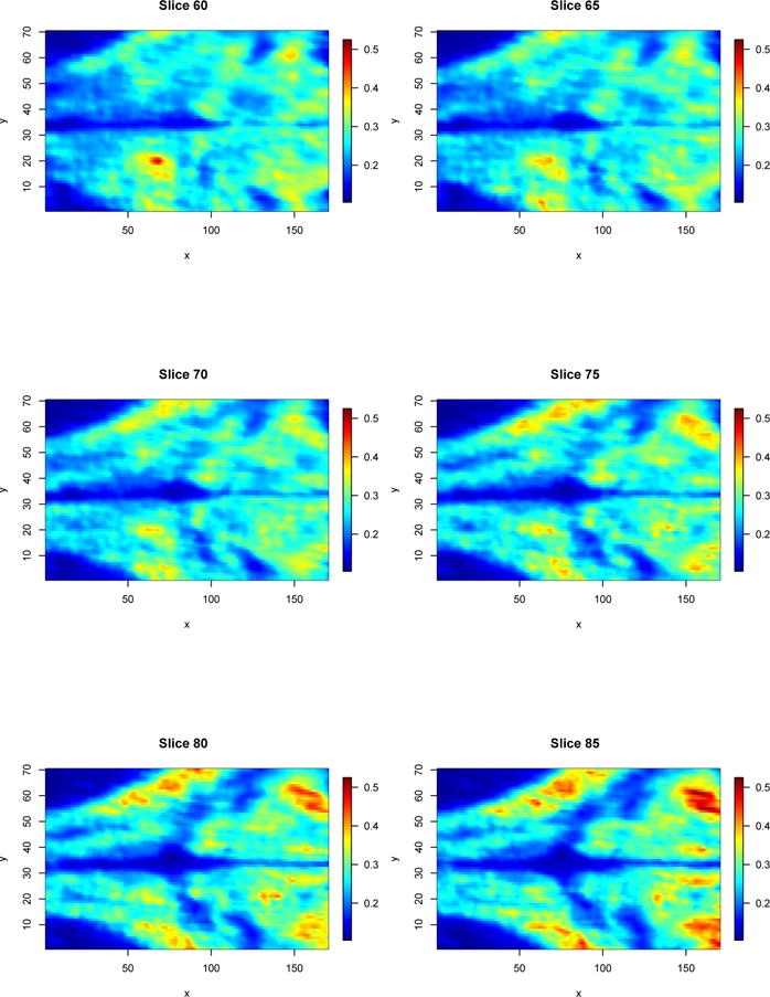
Time-averaged image of the the 60th to 85th z-slices (in increments of 5) of the zebrafish brain calcium imaging volume acquired using SCAPE microscopy. The legend on the right-hand sides indicate the average level of signal intensity at any particular voxel.

4.2 Data Analysis via Two-Stage Approach

All statistical analyses in this article are conducted within the R statistical environment [51] via the Microsoft Open 3.2.3 build. Data analysis is conducted using a mix of open source packages along with bespoke scripts. All computations are performed on a MacBook Pro (retina, 15-inch, early 2013) with a 2.4 GHz Intel Core i7 processor and 16 GB of DDR3 RAM. Computation times are measured using the proc.time function in the base package of R.

Imaging data were first converted from the raw time frames (ANDOR format) using a custom python script. Part of this pre-processing involves a conversion to MINC [52], a HDF5 based format such that we can more easily deal with datasets that approximate 1TB. Once in the MINC format, the data is then realigned within each volume, realigned for each time series, and intensity normalized using the MINC tools. This post-processing is performed on a ≈ 200 core Linux cluster using gridengine. A sub-section of the data are then extracted and converted to NIfTI format for statistical analysis. The NIfTI format images were read into R via the AnalyzeFMRI package [53]. Before initializing Stage 1 of our process, we firstly detrend the data. This is performed rapidly via the speedlm.fit function within the speedglm package [54]. The detrending is required due to the decaying effect of the fluorescence contrast over time, and is justified by the the imaged specimen being at rest. Using a d = 100 bases (i.e. a 98-node) B-spline system, the OLS estimates of the B-spline representation ${\stackrel{\sim }{\mathit{b}}}_i(i=1,\dots ,1785000)$ for Stage 1 of the procedure are quickly computed via the functions within the fda package [55]. An example sample of 10 time series ${\mathit{Z}}_i^T=(Z_i(1),\dots ,Z_i(2797))$ along with their estimated B-spline representations $\stackrel{\sim }{Y}(t)={\stackrel{\sim }{\mathit{b}}}_i^T\mathit{x}(t)(t=1,\dots ,2797)$ is visualized in Figure 2. Reading, detrending, and OLS estimation of every voxel in the volume was performed in a total computation time of 0.89 hours.

Figure 2.

Panel A visualizes 10 randomly sampled time series of intensities from the total of n = 1785000 voxels; different colors indicate the signals from different time series. Panel B visualizes the d = 100 basis (98-node) B-spline representations $\stackrel{\sim }{Y}(t)={\stackrel{\sim }{\mathit{b}}}_i^T\mathit{x}(t)$ for each of the 10 randomly sampled series; the colors correspond to those from Panel A.

Prior to conducting Stage 2 of the process, we firstly column normalize the obtained OLS estimates ${\stackrel{\sim }{\mathit{b}}}_i^T=\left({\stackrel{\sim }{b}}_{i1},\dots ,{\stackrel{\sim }{b}}_{id}\right)$. That is, for each j = 1, …, d, we normalize each of the jth column of coefficients ${\stackrel{\sim }{b}}_{1j}$, …, ${\stackrel{\sim }{b}}_{nj}$ by the respective mean and standard deviation. This is done to reduce the effects of differing dimensional scales. Upon normalization, the trimmed k-means algorithm is used to cluster the data. The TCLUST algorithm was applied via the tkmeans function from the tclust package [56]. Numbers of clusters in the set $\mathbb{K}=\{2,\dots ,50\}$ were considered, and the algorithm was repeated 20 times for each $k\in \mathbb{K}$, in order to mitigate against convergence to a spurious solution. The solution that maximized the objective (9) over all repetitions is taken to be the optimal k-cluster trimmed k-means estimator ${\stackrel{\sim }{\gamma }}_n^{[k]}$.

Using the objective sequence ${\mathcal{l}}_n\left({\stackrel{\sim }{\gamma }}_n^{[k]}\right)(k\in \mathbb{K})$, we utilize the capushe package [57] to implement the the DDSE method of [29]. Under the penalty pen (k) = dk, The slope heuristic is estimated to be $\stackrel{\sim }{\kappa }=1.335\times {10}^{-3}$. This results in the model selection rule

$$\widehat{k}=\arg \underset{k\in \mathbb{K}}{min}-\frac{{\displaystyle {\sum }_{i=1}^n\log }{\displaystyle {\sum }_{c=1}^k{\pi }_c{\varphi }_d}\left({\stackrel{\sim }{\mathit{b}}}_i;{\stackrel{\sim }{\mathit{\mu }}}_{cn}^{[k]},{\mathbf{I}}_d\right)}{n}+\frac{2.67kd}{{10}^3}.$$ (10)

Under Rule 10, the optimal number of clusters is determined to be $\widehat{k}=10$. Panel A of Figure 3 visualizes the average time taken to perform 20 repetitions of the TCLUST algorithm for each $k\in \mathbb{K}$; Panel B of Figure 3 visualizes the model selection criterion values $-n^{-1}{\mathcal{l}}_n\left({\stackrel{\sim }{\gamma }}_n^{[k]}\right)+2\stackrel{\sim }{\kappa }$ pen (k) for each considered k. The total computation time for 20 repetitions of the TCLUST algorithm for each k is 82.61 hours.

Figure 3.

Panel A visualizes the total amount of time (in seconds) taken to run the TCLUST algorithm for each $k\in \mathbb{K}(\mathbb{K}=\{2,\dots ,50\})$. Panel B visualizes the model selection criterion values for each k, as per Rule (10); the dotted line and circled point indicate the optimal value of the criterion and $\widehat{k}=10$, respectively.

4.3 Results

Upon reversing the normalization discussed in Section 4.2, we can write the $\widehat{k}=10$ cluster mean functions as ${\stackrel{\sim }{\mu }}_c(t)={\stackrel{\sim }{\mathit{\mu }}}_{cn}^T\mathit{x}(t)(c=1,\dots .10)$. A plot of the 10 cluster mean functions appears in Panel A of Figure 4; a frequency plot of the number of voxels that are allocated into each cluster (via Rule (8)) appears in Figure 4. From Figure 4, we notice that although the majority of mean functions appear parallel, there are a few that exhibit behavior that differs over time, and not simply differing in mean; for example, the c = 3 and c = 9 mean functions exhibit behavior that is substantially different to the others.

Figure 4.

Visualization of the $\widehat{k}=10$ mean functions ${\stackrel{\sim }{\mu }}_c(t)={\stackrel{\sim }{\mathit{\mu }}}_{cn}^T\mathit{x}(t)(c=1,\dots ,10)$ that are obtained via the TCLUST algorithm for trimmed k-means; the colors are as in Figure 5.

Visualizations of the clustering at the 60th to 85th z-slices (in increments of 5) are presented in Figure 5. From Figure 5, we can make some inferences regarding the nature of the voxels that are allocated to each cluster. For example, c = 1 can be inferred as background, lack of brain matter, or highly inactive neuronal material. Clusters c = 2, 3, 4, 5, 6, 7 can be inferred as edge effects on the interface between the background and the brain matter; the differences in these background effects may be explained by the various types of cellular materials such as membranes and tissues. Clusters c = 8; 9; 10 can be inferred as various types of brain matter. Furthermore, the cluster allocations in Figure 5 appears to be spatially coherent, thus indicating that the methodology is producing biologically meaningful results and not spurious allocations. The resulting clustering patterns require further investigation regarding their significance and interpretability. It is difficult to make a comment regarding the inferential significance of these particular cluster allocations at this stage, as the science regarding the analysis of such imaging protocols is still undergoing development. Further, we observe that the frequencies of the different clusters are quite varied, indicating that the process is able to identify both rare and common subpopulations of voxels.

Figure 5.

Cluster allocations (as per Rule (8)) of the 60th to 85th z-slices (in increments of 5) of the zebrafish brain calcium imaging volume. The legend on the right-hand sides indicate the cluster allocation and corresponds with the colors that are used in Figure 4.

5 Conclusions

High-speed volumetric microscopy technologies hold great potential for the investigation of neurological activity in animals; see for example [11]. The methodology for analysis of whole-volume calcium imaging data has not been well developed and especially not adapted to the Big Data pathologies that are inherit in the class of data. In this article, we have developed a model-based clustering method that addresses the problems of sparse sampling, high dimensionality, and spatial dependency, which are inherent in whole-volume calcium imaging data. Our methodology is a two-stage mixture model-based approach for the functional data analysis of time series that arise from calcium imaging experiments.

We derived a theoretical model under which our approach can be interpreted. The approach is demonstrated to coincide with the estimation of a GMM for OLS estimates of B-spline coefficients. The consistency (under data dependence) of the MLE of the model parameter that is required for the application of the approach is provided. For feasibility, a a simplification of the GMM is estimated using a trimmed k-means algorithm. A consistency result (under data dependence) is proven for the trimmed k-means estimators. This consistency result is novel and extends the previous results of [30] and [48] regarding the consistency of such estimators under independence of observations.

An example application of this method on a resting-state zebrafish calcium imaging dataset is presented. The computational timing of the approach, using freely-available open software, demonstrated the feasibility of the procedure. The outcome of the data analysis showed that the approach produces spatially coherent cluster allocations that are biologically interpretable and meaningful. Here, reasonable spatial contiguity is achieved without the need for direct account of spatial correlation.

Future directions for this research will involve the application of the approach on animals undergoing stimulation; such data will likely exhibit more functional asychronicities than those observed in the provided example. Computational times may be made faster via bespoke software for the problem, that are implemented in C, this may be incorporated in the current workflow via the Rcpp package [58]. The bespoke software may also make possible the application of less restrictive models for clustering.

Although spatial coherency is achieved in our obtained cluster allocations, such allocations can be made more spatially consistent via the application of an MRF (Markov random field) model, such as those successfully implemented in [59] and [24]. The MRF model can be applied as a third stage to the approach.

Finally, we note that the methodology that has been developed is not limited in application to calcium imaging studies but also any situation where large numbers of time series require clustering. Here, we say that data is large if conventional methodologies require an unreasonable amount of computational time. The settings that are suitable for our methodology include those where the time series may or may not be spatially correlated, and where they may or may not be sparsely sampled. Such situation occur frequently in modern scientific analysis. Some recent settings where our methodology may be applied in the future are towards the analysis of activity sensor data and functional magnetic resonance imaging data, such as those analyzed by [60] and [25], respectively.

Appendix

Description of Trimmed k-means

Let u₁, …, u_n be a realization of an ID (identically distributed) random sample U₁, …, U ∈ ℝ^d. Based on [48, Prop. 1], we can describe the α-trimmed k-means problem as the estimation of the mean vectors γ^T = (μ₁, …, μ_k), where μ_c (c = 1, …, k), via the maximization of the objective

$${\mathcal{L}}_n(\mathit{\gamma })=\frac{1}{n}{\displaystyle \sum _{i=1}^n{\displaystyle \sum _{c=1}^k{\delta }_c({\mathit{u}}_i;\gamma )\log D_c({\mathit{u}}_i;\mathit{\gamma })},}$$ (11)

where D_c (u; γ) = k⁻¹ϕ_d (u; μ_c, λI_d) and

$${\delta }_c(\mathit{u};\mathit{\gamma })=\mathbb{I}\left\{\mathit{u}\in \left\{\underset{c^{\prime }}{max}{D}_{c^{\prime }}(\mathit{u};\mathit{\gamma })=D_c(\mathit{u};\mathit{\gamma })\right\}\cap \left\{D_c(\mathit{u};\mathit{\gamma })\ge R(\mathit{\gamma })\right\}\right\}.$$ (12)

Here λ > 0 is a fixed constant, $\mathbb{I}(A)$ equals 1 if A is true and 0 otherwise, and R (γ) = inf_v {G (v; γ) ≥ α}, where $G(v;\mathit{\gamma })=\mathbb{P}({max}_c{D}_c(\mathit{u};\mathit{\gamma })\le v)$ under the distribution of U₁. Call the α-trimmed k-means estimate ${\stackrel{\sim }{\mathit{\gamma }}}_n^T=({\stackrel{\sim }{\mathit{\mu }}}_{n1},\dots ,{\stackrel{\sim }{\mathit{\mu }}}_{nk})$.

Upon inspecting the objective (11), we observe that (12) sets the contribution of all observations u_i that have max_c D_c (u_i; γ) values below the α-quantile to 0; traditionally, the observations below the α-quantile are seen to be outliers. Thus, only (1 − α) × 100% of the data contributes non-zero values to the computation of the objective. This explains the faster computational speed of the trimmed k-means over its untrimmed counterpart, when α is sufficiently large. With respect to the size of data in our application, we found α = 0.9 to be reasonable.

TCLUST Algorithm

Like the k-means problem, the α-trimmed k-means problem is combinatorial and thus difficult to solve exactly. An approximate solution for maximizing (11) is to use the TCLUST algorithm. Here, we adapt the description of the TCLUST algorithm (given in [48, Sec. 3]) for the α-trimmed k-means problem.

Let γ⁽⁰⁾ denote some randomized initialization of the vector γ, and let ${\mathit{\gamma }}^{(r)T}=\left({\mathit{\mu }}_1^{(r)},\dots ,{\mathit{\mu }}_k^{(r)}\right)$ denote the rth iterate of the algorithm. At the (r + 1) th iterate of the algorithm, perform the steps:

• 1. Compute $d_i^{(r)}={max}_c{D}_c({\mathit{u}}_i;{\mathit{\gamma }}^{(r)})$ and store the set of u_i with the ⎿n (1 − α)⏌ largest $d_i^{(r)}$ values in the set ${ℍ}^{(r+1)}$.

• 2. Split ${ℍ}^{(r+1)}$ into sets ${ℍ}_1^{(r+1)}$, …, ${ℍ}_k^{(r+1)}$, where

$${ℍ}_c^{(r+1)}=\{{\mathit{u}}_i\in {ℍ}^{(r+1)}:D_c\left({\mathit{u}}_i;{\mathit{\gamma }}^{(r)}\right)=d_i^{(r)}\}.$$

• 3. For each c = 1, …, k, compute the updates

$${\mathit{\mu }}_c^{(r+1)}={|{ℍ}_c^{(r+1)}|}^{-1}{\displaystyle \sum _{i=1}^n{\mathit{u}}_i\mathbb{I}\left\{{\mathit{u}}_i\in {ℍ}_c^{(r+1)}\right\}}.$$

Here ⎿x⏌ is the floor of x ∈ ℝ. Steps 1–3 are repeated until some convergence criterion is met upon which the final iterate is declared the α-trimmed k-means estimator ${\stackrel{\sim }{\mathit{\gamma }}}_n$. In this article, we follow the default option of the tkmeans function and terminate the algorithm after 20 iterations.

Theoretical Considerations

The consistency of the α-trimmed k-means estimator ${\stackrel{\sim }{\mathit{\gamma }}}_n$ is established for the case of independent and identically distributed random variables in [48]; see also [30]. Due to the application to CI, we require that the α-trimmed k-means estimator be consistent for data with some dependence structure. Let ⪯ denote the lexicographic order relation in ℝ^d (cf. [61, Example 2.1.10 (3)]), and let Γ = {γ ∈ ℝ^kd : μ₁ ⪯ … ⪯ μ_k}. Further, let $l(\mathit{u};\mathit{\gamma })={\displaystyle {\sum }_{c=1}^k{\delta }_c(\mathit{u};\mathit{\gamma })\log D_c}(\mathit{u};\mathit{\gamma })$. The following proposition establishes one such result.

Proposition 3

Let U₁, …, U_n ∈ ℝ^d be an ID and stationary ergodic (or strong-mixing) random sample from a continuous distribution and assume that |cov (U₁)| < ∞. Assume that there exists some γ₀ ∈ Γ such that for every open subset $\mathcal{G}\subset \mathrm{\Gamma }$, ${\mathit{\gamma }}_0\in \mathcal{G}$ implies that $\mathbb{E}l({\mathit{U}}_1;{\mathit{\gamma }}_0)>{\sup }_{\mathit{\gamma }\in \mathrm{\Gamma }\backslash \mathcal{G}}\mathbb{E}l({\mathit{U}}_1;\mathit{\gamma })$. If ${\stackrel{\sim }{\mathit{\gamma }}}_n\in \mathrm{\Gamma }$ is a sequence of estimators such that ${\stackrel{\sim }{\mathit{\gamma }}}_n=\arg {max}_{\mathit{\gamma }\in \mathrm{\Gamma }}{\mathcal{L}}_n(\gamma )$, then ${\stackrel{\sim }{\mathit{\gamma }}}_n\stackrel{P}{\to }{\gamma }_0$

Proof

We invoke the M-estimator theorem of [62, Thm. 2.12], which requires we establish that

$$\underset{\mathit{\gamma }\in \mathrm{\Gamma }}{\sup }|{\mathcal{L}}_n(\mathit{\gamma })-\mathbb{E}l({\mathit{U}}_1;\mathit{\gamma })|\stackrel{P}{\to }0.$$

Under the ID stationary ergodic (or strong-mixing) condition, we can use the ULLN of [38, Thm. 5] by verifying that $\mathbb{E}l({\mathit{U}}_1;\mathit{\gamma })<\infty$ (which also verifies the use of an appropriate law of large numbers; e.g. [37, Thm. 3.34]). Since δ_c (u₁; γ) are binary, we require that $\mathbb{E}\log D_c(\mathit{u};\mathit{\gamma })$ be finite for each c. Since log D_c (u; γ) is nonlinear in u via only quadratic terms, we have $\mathbb{E}\log D_c(\mathit{u};\mathit{\gamma })<\infty$ and hence $\mathbb{E}l(\mathit{u};\mathit{\gamma })<\infty$, under the assumption that |cov (U₁)| < ∞. □

Remark 8

The constraint of the parameter space to Γ is require to break the symmetries of potential solutions. Without the restriction, the assumption that there exists some γ₀ ∈ Γ such that for every open subset $\mathcal{G}\subset \mathrm{\Gamma }$, ${\mathit{\gamma }}_0\subset \mathcal{G}$ implies that $\mathbb{E}l({\mathit{U}}_1;{\mathit{\gamma }}_0)>{\sup }_{\mathit{\gamma }\in \mathrm{\Gamma }\backslash \mathcal{G}}\mathbb{E}l({\mathit{U}}_1;\mathit{\gamma })$ cannot hold, since there will always be a $\mathit{\gamma }\in \mathrm{\Gamma }\backslash \mathcal{G}$ such that $\mathbb{E}l({\mathit{U}}_1;{\mathit{\gamma }}_0)=\mathbb{E}l({\mathit{U}}_1;\mathit{\gamma })$. The lexicographic ordering restriction is similar to that which is used by [63], in order to break symmetries in mixture of experts models.

Remark 9

As with Proposition 2, an M-dependence assumption can be used to enforce strong-mixing; see Remark 5. However, similarly to Remark 6, M-dependence may be difficult to establish if all dimensions of the calcium imaging is allowed to extend infinitely. An alternative theorem based on the results of [41] can be used instead in such a case.

References

- 1.Burgoyne RD. Neuronal calcium sensor proteins: generating diversity in neuronal Ca2+ signalling. Nature Reviews Neuroscience. 2007;8:182–193. doi: 10.1038/nrn2093. [DOI] [PMC free article] [PubMed] [Google Scholar]
- 2.Denk W, Yuste R, Svoboda K, Tank DW. Imaging calcium ddynamic in dendritic spines. Current Opinion in Neurobiology. 1996;6:372–378. doi: 10.1016/s0959-4388(96)80122-x. [DOI] [PubMed] [Google Scholar]
- 3.Yasuda R, Nimchinsky EA, Scheuss V, Pologruto TA, Oertner TG, Sabatini BL, et al. Imaging calcium concentration ddynamic in small neuronal compartments. Science’s STKE. 2004;2004(219) doi: 10.1126/stke.2192004pl5. [DOI] [PubMed] [Google Scholar]
- 4.Chen TW, Wardill TJ, Sun Y, Pulver SR, Renninger SL, Baohan A, et al. Ultrasensitive fluorescent proteins for imaging neuronal activity. Nature. 2013;499:295–300. doi: 10.1038/nature12354. [DOI] [PMC free article] [PubMed] [Google Scholar]
- 5.Stewart AM, Ullmann JF, Norton WH, Parker MO, Brennan CH, Gerlai R, et al. Molecular psychiatry of zebrafish. Molecular Psychiatry. 2015;20:2–17. doi: 10.1038/mp.2014.128. [DOI] [PMC free article] [PubMed] [Google Scholar]
- 6.Ullmann JF, Calamante F, Collin SP, Reutens DC, Kurniawan ND. Enhanced characterization of the zebrafish brain as revealed by super-resolution track-density imaging. Brain Structure and Function. 2015;220:457–468. doi: 10.1007/s00429-013-0667-7. [DOI] [PMC free article] [PubMed] [Google Scholar]
- 7.Thiele TR, Donovan JC, Baier H. Descending control of swim posture by a midbrain nucleus in zebrafish. Neuron. 2014;83:679–691. doi: 10.1016/j.neuron.2014.04.018. [DOI] [PMC free article] [PubMed] [Google Scholar]
- 8.Thompson AW, Vanwalleghem GC, Heap LA, Scott EK. Functional profiles of visual-, auditory-, and water flow-responsive neurons in the zebrafish tectum. Current Biology. 2016;26:743–754. doi: 10.1016/j.cub.2016.01.041. [DOI] [PubMed] [Google Scholar]
- 9.Ahrens MB, Orger MB, Robson DN, Li JM, Keller PJ. Whole-brain functional imaging at celcell resolution using light-sheet microscopy. Nature Methods. 2013;10:413–420. doi: 10.1038/nmeth.2434. [DOI] [PubMed] [Google Scholar]
- 10.Marquart GD, Tabor KM, Brown M, Strykowski JL, Varshney GK, LaFave MC, et al. A 3D searsearch database of transgenic zebrafish Gal4 and Cre lines for functional neuroanatomy studies. Frontiers in Neural Circuits. 2015;9 doi: 10.3389/fncir.2015.00078. [DOI] [PMC free article] [PubMed] [Google Scholar]
- 11.Bouchard MB, Voleti V, Mendes CS, Lacefield C, Grueber WB, Mann RS, et al. Swept confocally-aligned planare excitation (SCAPE) microscopy for high-speed volumetric imaging of behaving organisms. Nature Photonics. 2015;9:113–119. doi: 10.1038/nphoton.2014.323. [DOI] [PMC free article] [PubMed] [Google Scholar]
- 12.Chen M, Mao S, Liu Y. Big Data: a survey. Mobile Networks and Applications. 2014;19:171–209. [Google Scholar]
- 13.Liao TW. Clustering of time series data—a survey. Pattern Recognition. 2005;38:1857–1874. [Google Scholar]
- 14.Esling P, Agon C. Time-series data mining. ACM Computing Surveys. 2012;45:12:1–12:34. [Google Scholar]
- 15.Ramsay JO, Silverman BW. Functional Data Analysis. New York: Springer; 2005. [Google Scholar]
- 16.Gaffney S, Smyth P. Trajectory clustering with mixtures of regression models. Proceedings of the fifth ACM SIGKDD International Conference on Knowledge Discovery and Data Mining. 1999 [Google Scholar]
- 17.James GM, Sugar CA. Clustering for sparsely sampled functional data. Journal of the American Statistical Association. 2003;98:397–408. [Google Scholar]
- 18.Celeux G, Martin O, Lavergne C. Mixture of linear mixed models for clustering gene expression profiles from repeated microarray experiments. Statistical Modelling. 2005;5:243–267. [Google Scholar]
- 19.Ng SK, McLachlan GJ, Ben-Tovim KWL, Ng SW. A mixture model with random-effects components for clustering correlated gene-expression profiles. Bioinformatics. 2006;22:1745–1752. doi: 10.1093/bioinformatics/btl165. [DOI] [PubMed] [Google Scholar]
- 20.Wang K, Ng SK, McLachlan GJ. Clustering of time-course gene expression profiles using normal mixed models with autoregressive random effects. BMC Bioinformatics. 2012;13:300. doi: 10.1186/1471-2105-13-300. [DOI] [PMC free article] [PubMed] [Google Scholar]
- 21.Ng SK, McLachlan GJ. Mixture of random effects models for clustering multilevel growth trajectories. Computational Statistics and Data Analysis. 2014;71:43–51. [Google Scholar]
- 22.Nguyen HD, McLachlan GJ, Wood IA. Mixture of spatial spline regressions for clustering and classification. Computational Statistics and Data Analysis. 2016;93:76–85. [Google Scholar]
- 23.Xiong Y, Yeung DY. Time series clustering with ARMA mixtures. Pattern Recognition. 2004;37:1675–1689. [Google Scholar]
- 24.Nguyen HD, McLachlan GJ, Ullmann JFP, Janke AL. Spatial clustering of time-series via mixture of autoregressions models and Markov Random Fields. Statistica Neerlandica. 2016;70:414–439. [Google Scholar]
- 25.Nguyen HD, McLachlan GJ, Orban P, Bellec P, Janke AL. Maximum pseudolikelihood estimation for model-based clustering of time series data. Neural Computation. 2017;29:990–1020. doi: 10.1162/NECO_a_00938. [DOI] [PubMed] [Google Scholar]
- 26.Nguyen HD, McLachlan GJ, Ullmann JFP, Janke AL. Faster functional clustering via Gaussian mixture models. 2016 arXiv:160805481. [Google Scholar]
- 27.McLachlan GJ, Peel D. Finite Mixture Models. New York: Wiley; 2000. [Google Scholar]
- 28.Schwarz G. Estimating the dimensions of a model. Annals of Statistics. 1978;6:461–464. [Google Scholar]
- 29.Baudry JP, Maugis C, Michel B. Slope heuristic: overview and implementation. Statistics and Computing. 2012;22:455–470. [Google Scholar]
- 30.Cuesta-Albertos JA, Gordaliza A, Matran C. Trimmed k-means: an attempt to robustify quantizers. Annals of Statistics. 1997;25:553–576. [Google Scholar]
- 31.Abraham C, Cornillon PA, Matzner-Lober E, Molinari N. Unsupervised curve clustering using B-splines. Scandinavian Journal of Statistics. 2003;30:581–595. [Google Scholar]
- 32.Peng J, Muller HG. Distance-based clustering of sparsely observed stochastic processes, with applications to online auctions. Annals of Applied Statistics. 2008;2:1056–1077. [Google Scholar]
- 33.Dempster AP, Laird NM, Rubin DB. Maximum likelihood from incomplete data via the EM algorithm. Journal of the Royal Statistical Society Series B. 1977;39:1–38. [Google Scholar]
- 34.de Boor C. A Practical Guide to Splines. New York: Springer; 2001. [Google Scholar]
- 35.Seber GAF. A Matrix Handbook For Statisticians. New York: Wiley; 2008. [Google Scholar]
- 36.Amemiya T. Advanced Econometrics. Cambridge: Harvard University Press; 1985. [Google Scholar]
- 37.White H. Asymptotic Theory For Econometricians. San Diego: Academic Press; 2001. [Google Scholar]
- 38.Andrews DWK. Generic uniform convergence. Econometric Theory. 1992;8:241–257. [Google Scholar]
- 39.Bradley RC. Basic properties of strong mixing conditions. A survey and some open questions. Probability Surveys. 2005;2:107–144. [Google Scholar]
- 40.Bradley RC. A caution on mixing conditions for random fields. Statistics and Probability Letters. 1989;8:489–491. [Google Scholar]
- 41.Jenish N, Prucha IR. Central limit theorems and uniform laws of large nnumber for arrays of random fields. Journal of Econometrics. 2009 doi: 10.1016/j.jeconom.2009.02.009. [DOI] [PMC free article] [PubMed] [Google Scholar]
- 42.Hartigan JA, Wong MA. Algorithm AS 136: A k-means clustering algorithm. Journal of the Royal Statistical Society Series C. 1979;28:100–108. [Google Scholar]
- 43.McLachlan GJ. Discriminant Analysis And Statistical Pattern Recognition. New York: Wiley; 1992. [Google Scholar]
- 44.Press WH, Teukolsky SA, Vetterling WT, Flannery BP. Numerical Recipes: The Art of Scientific Computing. Cambridge: Cambridge University Press; 2007. [Google Scholar]
- 45.Massart P. Concentration Inequalities and Model Selection. New York: Springer; 2007. [Google Scholar]
- 46.Birge L, Massart P. Minimal penalties for Gaussian model selection. Probability Theory and Related Fields. 2007;138:33–73. [Google Scholar]
- 47.Baudry JP, Maugis C, Michel B. Slope heuristic: overview and implementation. INRIA. 2010 hal-00461639. [Google Scholar]
- 48.Garcia-Escudero LA, Gordaliza A, Matran C, Mayo-Iscar A. A general trimming approach to robust cluster analysis. Annals of Statistics. 2008 [Google Scholar]
- 49.Hubert L, Arabie P. Comparing partitions. Journal of Classification. 1985;2:193–218. [Google Scholar]
- 50.Vladmirov N, Mu Y, Kawashima T, Bennett DV, Yang CT, Looger LL, et al. Light-sheet functional imaging in fictively behaving zebrafish. Nature Methods. 2014;11:883–884. doi: 10.1038/nmeth.3040. [DOI] [PubMed] [Google Scholar]
- 51.R Core Team. R: a language and environment for statistical computing. 2013 [Google Scholar]
- 52.Vincent RD, Janke A, Sled JG, Baghdadi L, Neelin P, Evans AC. MINC 2.0: a modality independent format for multidimensional medical images. 10th Annual Meeting of the Organization for Human Brain Mapping. 2003 [Google Scholar]
- 53.Bordier C, Dojat M, de Micheaux PL. Temporal and spatial independent component analysis for fMRI data sets embedded in the AnalyzeFMRI R package. Journal of Statistical Software. 2011;44:1–24. [Google Scholar]
- 54.Enea M. speedglm: fitting linear and generalized linear models to large data sets. 2015 [Google Scholar]
- 55.Ramsay JO, Hooker G, Graves S. Functional Data Analysis with R and MATLAB. New York: Springer; 2009. [Google Scholar]
- 56.Fritz H, Garcia-Escudero LA, Mayo-Iscar A. TCLUST: an R package for a trimming approach to cluster analysis. Journal of Statistical Software. 2012;47:1–26. [Google Scholar]
- 57.Arlot S, Brault V, Baudry JP, Maugis C, Michel B. capushe: CAlibrating Penalities Using Slope HEuristics. 2015 [Google Scholar]
- 58.Eddelbuettel D. Seamless R and C++ Integration with Rcpp. New York: Springer; 2013. [Google Scholar]
- 59.Nguyen HD, McLachlan GJ, Cherbuin N, Janke AL. False discovery rate control in magnetic resonance imaging studies via Markov random fields. IEEE Transactions on Medical Imaging. 2014;33:1735–1748. doi: 10.1109/TMI.2014.2322369. [DOI] [PubMed] [Google Scholar]
- 60.Trabelsi D, Mohammed S, Chamroukhi F, Oukhellou L, Amirat Y. An unsupervised approach for automatic activity recognition based on hidden Markov model regression. IEEE Transactions on Automation Science and Engineering. 2013;10:829–835. [Google Scholar]
- 61.Khan AA, Tammer C, Zalinescu C. Set-valued Optimization. New York: Springer; 2015. [Google Scholar]
- 62.Kosorok MR. Introduction to Empirical Processes and Semiparametric Inference. New York: Springer; 2008. [Google Scholar]
- 63.Jiang W, Tanner MA. On the identifiability of mixture-of-experts. Neural Networks. 1999;12:1253–1258. doi: 10.1016/s0893-6080(99)00066-0. [DOI] [PubMed] [Google Scholar]