Substance and Artifact in the Higher-Order Factors of the Big Five

Abstract

J. M. Digman (1997) proposed that the Big Five personality traits showed a higher-order structure with 2 factors he labeled α and β. These factors have been alternatively interpreted as heritable components of personality or as artifacts of evaluative bias. Using structural equation modeling, the authors reanalyzed data from a cross-national twin study and from American cross-observer studies and analyzed new multimethod data from a German twin study. In all analyses, artifact models outperformed substance models by root-mean-square error of approximation criteria, but models combining both artifact and substance were slightly better. These findings suggest that the search for the biological basis of personality traits may be more profitably focused on the 5 factors themselves and their specific facets, especially in monomethod studies.

In 1997, Digman showed that across several data sets and instruments, scales measuring the Big Five factors—as the higher-order dimensions of the five-factor model (FFM; McCrae & John, 1992) of personality traits are commonly called—tended to show a consistent pattern of intercorrelations that could be summarized in terms of two even higher-order factors, which he called α, or socialization, and β, or personal growth. The former was defined by low Neuroticism (N) and high Agreeableness (A) and Conscientiousness (C); the latter was defined by Extraversion (E) and Openness (O). Digman interpreted these factors in terms of constructs from classic theories of personality. For example, he related the self-actualization theories of Rogers (1961) and Maslow (1954) to the outgoing, adventurous, and creative traits associated with β. Much of the appeal of his work lies in his efforts to integrate personality structure with personality theories.

Independently, Becker (1999) reported higher-order factor analyses of German inventories that suggested two factors he labeled Mental Health and Behavior Control. DeYoung, Peterson, and Higgins (2002) argued that these factors were a rotation of Digman’s (1997) factors, such that α is intermediate between Mental Health and high Behavior Control, whereas β lies between Mental Health and low Behavior Control. DeYoung et al. relabeled α as Stability and β as Plasticity and proposed neurobiological bases for them. Jang et al. (2006) reported behavior genetic analyses of domain scales from the Revised NEO Personality Inventory (NEO-PI-R; Costa & McCrae, 1992) in Canadian, German, and Japanese samples that suggested that α and β might be heritable, although in the German and Japanese samples, α was defined only by low N and high C. The presence of genetic associations seems to imply that α and β are substantive factors of personality, although Jang et al. pointed out that these genetic effects so far have been demonstrated in only one instrument, the NEO-PI-R.

However, the view that α and β are substantive constructs at a higher order than the Big Five has also been challenged. An alternative is that they are method artifacts and that the five factors are themselves orthogonal. In support of that position, McCrae and Costa (1989) showed that there is slightly greater cross-observer agreement between orthogonal factor scores than between oblique factor scores or raw domain scores. Similarly, Biesanz and West (2004) compared self-reports, peer ratings, and parental ratings on an adjective measure of the Big Five and concluded that “observed correlations among Big Five traits are the product of informant-specific effects” (p. 870); that is, different domains were correlated within each data source but were unrelated across sources.

Such informant-specific effects are generally interpreted as method artifacts, biases that contribute to observed scores because of the method used rather than as a reflection of the true score. Two accounts of the nature of these artifacts have been proposed. McCrae and Costa (1995) reported a joint factor analysis of the NEO-PI-R and Tellegen, Grove, and Waller’s (1991) Inventory of Personal Characteristics #7 (IPC7). The IPC7 includes versions of the Big Five factors along with scales assessing positive valence (PV; flawless, outstanding vs. ordinary, unremarkable) and negative valence (NV; sick, immoral, deceitful vs. fair-minded, unselfish). In a five-factor solution, PV showed strong loadings on the E and O factors, whereas NV had a positive loading on the N factor and negative loadings on the E, A, and C factors. McCrae and Costa (1999) subsequently argued that β could reflect the operation of PV bias: People who are inclined to describe themselves in glowing terms may exaggerate their standing on E and O, creating a spurious correlation between them. Because different raters would presumably not share PV biases, E and O would appear to be orthogonal in cross-observer studies.¹ Similarly, α could be due to (low) NV.

Paulhus and John (1998) have also argued that the intercorrelation of Big Five scales “suggests the intrusion of two evaluative superfactors” (p. 1040), which they labeled Moralistic and Egoistic Biases, the former corresponding roughly to Digman’s (1997) α and the latter to his β (although N does not clearly define either superfactor). Although Paulhus and John described these as biases in self-perception, the informant-specific effects noted by Biesanz and West (2004) suggest that the same biases may operate in observers.

Other researchers, however, have argued that PV and NV are, at least in part, substantive factors (Benet-Martínez & Waller, 2002; Durrett & Trull, 2005), so it is probably wise to distinguish them from the within-informant biases to which they may be related. DeYoung (2006) identified both across-informant and within-informant sources of correlations among the Big Five, which might be interpreted as substance and artifact, respectively. In most of DeYoung’s samples, the within-informant effects, or uniquenesses, formed two factors, one related to A, C, and low N and the other related to E and O; he also found that these two factors were themselves correlated, consistent with a global evaluative dimension. In the present study, we designate these as latent variables A-bias and B-bias, respectively, and we allow them to be correlated.

Comparing Models

To compare substantive and artifactual interpretations of α and β, it is necessary to have at least two independent but related assessments of the five factors. The cross-observer design of Biesanz and West (2004) is one obvious approach, but it is also possible to compare substance and artifact models in behavior genetic samples, where we can determine the extent to which traits independently assessed in different twins are heritable and whether their correlation is attributable to a shared genetic basis or to artifact (see Jang, 2005, for a full description). This makes it possible to reanalyze the data of Jang et al. (2006), who provided evidence for a substantive interpretation but did not explicitly model an artifactual interpretation, and to estimate the relative contributions of both substance and artifact. Here, we present results of such a comparison.

In Study 1, we compare four models: a baseline model that assumes that the five factors are orthogonal, a substance model that includes heritable α and β, an artifact model that includes correlated A- and B-bias, and a full model with both substance and artifact. Comparisons of model fit allow an assessment of how well these competing hypotheses explain the observed data. In terms of the observed correlations of E and O, the baseline model implies that they are uncorrelated, the substance model implies they are correlated both within and across twins and to the same degree, the artifact model implies that they are correlated only within twins, and the full model assumes that they are correlated both within and across twins but more strongly within twins.

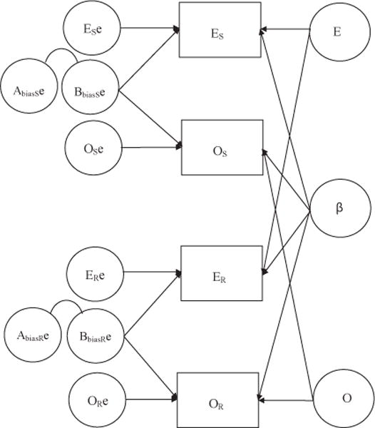
These four models are illustrated in Figure 1, a set of path diagrams representing possible influences on observed E and O scores in pairs of monozygotic (MZ) twins. On the right in each panel are possible genetic causes. In Panel A, the baseline model is presented, in which there are independent genetic causes (Eg and Og) of observed E and O scores; the remaining variance in observed scores is attributed to uncorrelated error terms (E₁e to O₂e) on the left. Panel B represents the substance model, in which β is added and is hypothesized to influence both E and O scores and thus cause their covariation. This model suggests that E and O scores will covary both within and across twins. Panel C depicts the artifact model, in which the covariation of E and O scores is attributed to B-bias and is found only within twins; B-bias for Twin 1 is uncorrelated with B-bias for Twin 2. However, B-bias for each twin is allowed to correlate with A-bias for that twin, the correlation representing a general evaluative bias.² The latent variables on the left include both error of measurement and any influences on true scores that are not shared by twins. It is important to note that this model assumes that there is no shared environmental influence, an assumption justified both by analyses of this data set (Yamagata et al., 2006) and by the broader literature on the behavior genetics of personality (Bouchard & Loehlin, 2001; Plomin & Daniels, 1987), where both twin and adoption studies have consistently failed to find shared environmental effects for personality traits in adults.

Figure 1.

Path diagram of influences on observed Extraversion (E) and Openness (O) domains in monozygotic twins. Variables with subscript “1” refer to the first twin; those with subscript “2” refer to the second twin. The letters g and e designate additive genetic and nonshared environmental influences, respectively. Panel A presents the baseline model, Panel B the substance model, Panel C the artifact model with correlated A_bias and B_bias, and Panel D the full model with correlated A_bias and B_bias, including path coefficients from Table 1. B_bias = within-twin bias; β = Digman’s (1997) personal growth factor.

A similar diagram can be constructed for N (reflected to represent the emotional stability component of α), A, and C. We estimate latent variables contributing to all five factors in each model together, with the assumption that all latent variables are independent (except for A- and B-bias). For simplicity, Figure 1 represents the case for MZ twins, but by specifying that dizygotic (DZ) twins share half their genes, it is also possible to include DZ twin data in a combined model.

The Study 1 design, in which self-reports from twins are analyzed, provides a clear test of the relative roles of substance and artifact if, as the model suggests, the genetic effect is substantive and the nonshared environmental effect (which includes error) is artifactual. Those are straightforward and plausible assumptions, but they are not necessarily true. An alternative hypothesis for β is that twins inherit a shared tendency toward B-bias. Such a shared bias would inflate the E and O scores of both twins. Thus, the latent variable in Figure 1 labeled βg could also be labeled B_biasg. Similarly, it is possible to propose an alternative hypothesis for B-bias: Instead of being an unshared bias, it may reflect unique life experiences that have contributed substantively to both E and O, but separately for each twin. Thus, the latent variables labeled B_biase could also be interpreted as βe. Monomethod twin studies separate genetic from environmental effects, but they do not unambiguously separate substance from artifact.

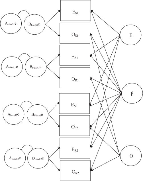
To separate substance from artifact more clearly, in Study 2 we examine cross-observer data using a parallel design. Self-reports and observer ratings were available for two samples (adult and adolescent), and cross-observer agreement can be interpreted as evidence of substantive influences. In Figure 2, which illustrates the full model, influences on the true scores (as operationally defined by cross-observer agreement in these data) are given on the right; these include those that affect E and O separately across methods and β, which is hypothesized to affect both domains across methods. In this design, the underlying causes of traits (genetic, shared environmental, or nonshared environmental) are not distinguished: Whatever the causes are, if they affect the true score of the traits, then they should appear in both self-reports and observer ratings. If influences on true scores are on the right, then variables on the left must influence error, both random and systematic. Systematic error that is informant specific and that contributes to both E and O scores is labeled B_bias. This design yields information on the relative contributions of substance and artifact to the covariation of Big Five scores but does not explain their origins. A stronger design would used data from three or more raters from different categories (e.g., self-reports, spouse ratings, peer ratings; see Cole, Ciesla, & Steiger, 2007).

Figure 2.

Path diagram of influences on self-reported and observer-rated Extraversion (E) and Openness (O) domains, full model with correlated A_bias and B_bias. Variables with subscript “S” refer to self-reports; those with subscript “R” refer to observer ratings. The letter e designates error or systematic bias terms. B_bias = within-informant bias; β = Digman’s (1997) personal growth factor.

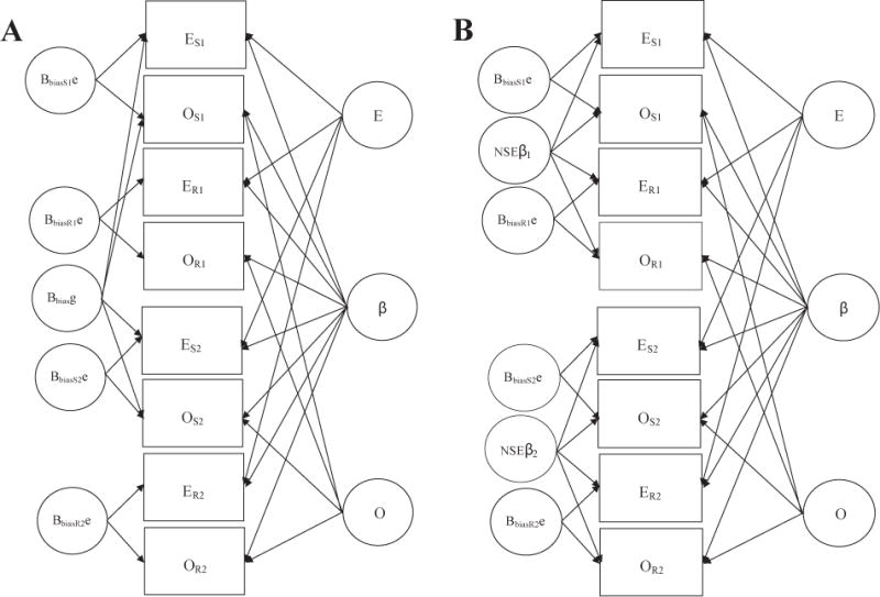
Study 3 combines aspects of both these designs and is correspondingly more informative (see Bartels, Boomsma, Hudziak, van Beijsterveldt, & van den Oord, 2007, for other genetically informative multirater designs). Both self-reports and observer ratings on the German NEO-PI-R were available for a sample of MZ and DZ twins. The basic model for β is shown in Figure 3 for MZ twins, with Twin 1 data represented in the top four boxes and Twin 2 data in the bottom four boxes. The variables on the right reflect true score influences (as operationalized by cross-observer agreement) shared by both twins, which include genetic influences on E and on O and, through β, on both E and O. The variables on the left contribute to correlations between E and O that are not shared across method or across twins and thus can reasonably be interpreted as artifact. Not shown in Figure 3 are latent variables representing the nonshared environment plus error.

Figure 3.

Path diagram of influences on self-reported and observer-rated Extraversion (E) and Openness (O) domains in monozygotic twins, full model with correlated A_bias and B_bias. Variables with subscript “S” refer to self-reports; those with subscript “R” refer to observer ratings. Variables with subscript “1” refer to the first twin; those with subscript “2” refer to the second twin. The letter e designates systematic bias. Error specific to twin, domain, and method of measurement is not shown in the model. B_bias = within-informant bias; β = Digman’s (1997) personal growth factor.

Two variations on this model are also informative. In the first, we add new latent variables reflecting possible genetic influences on the artifacts of A- and B-bias. These variables would affect the self-reports of both twins but not observer ratings. (Note that because different observers rated the twins in each pair, latent variables reflecting rater bias cannot be estimated.) In the second variation, we consider the possibility of substantive nonshared environmental effects. These latent variables would affect both self-reports and ratings of a twin but would not affect assessments of the other twin. Significant effects for these variables would demonstrate consensually validated nonshared environmental effects.

Substance and Artifact Reconsidered

To this point, we have assumed that cross-observer agreement is evidence of the consensual validation of traits and their associations. However, researchers concerned with social perception (see Funder & West, 1993) have pointed out that consensus among raters may be attributable instead to shared but unfounded cognitive schemas. In particular, we might hypothesize that all people share the mistaken assumption that extraverts are open to experience and open people are extraverted. An individual who accurately perceived that a target was high in E would then exaggerate the target’s O score, and vice versa. A similar schema might relate perceptions of N, A, and C. We can label these schemas as α′ and β′.

There is indirect evidence that such shared schemas exist. Sneed, McCrae, and Funder (1998, Study 1) asked several groups of students to rate how well 30 adjectives served as indicators of each factor. Students gave the highest rating to the correct factor in 29 of 30 cases, suggesting that they understood the constructs represented by the factors. However, there was also evidence of poor discrimination among the five factors. For example, on a scale from −1.0 to 1.0, the mean rating for enthusiastic as an indicator of E was .90, but its rating as an indicator of O was .64; reliable was deemed a good indicator of C (.86) but also of N (−.52) and A (.64). A factor analysis of mean ratings for the five factors showed one large evaluative factor (corresponding to the general evaluative factor identified by DeYoung, 2006), but if two factors were extracted and rotated, the first was defined by N (−.84), A (.75), and C (.92) and the second by E (.94) and O (.85). Thus, α′ and β′ can be found in students’ explicit conceptions of traits. Such preconceptions might easily color their ratings of a real target’s personality.

The same logic would apply to self-reports, and twins who in fact shared personality traits and accurately perceived them would be led to the same biased assessment of other traits, making α′ and β′ in the self-reports of twins appear to be heritable. This hypothesis proposes that there is a universal tendency to confound Big Five traits at a higher-order level, akin to the implicit personality theory that operates at the level of the FFM (see McCrae, Jang, Livesley, Riemann, & Angleitner, 2001). In the same way, unfounded schemas shared between self-reporters and observers could give the appearance that α′ and β′ are consensually validated.

In the language of structural equation modeling (SEM), these are mediated models in which, for example, latent E and O influence the latent mediator β′ and thus have indirect influences on observed E and O scores in addition to their direct influences (see Figure 4). In this model, β′ does not represent a source of true-score variance in personality; instead, it represents a feature of person perception (a cognitive schema) that influences personality ratings. β represents the true source of covariation between E and O (if any). Such indirect paths can be included in an SEM analysis of correlations, but, unfortunately, this model is underidentified and thus the paths can assume any values consistent with the principle that the sum of squared path coefficients to β′ must equal 1.0. Further, if paths a and c are constrained to be equal, then the fit of all these mediated models is identical to that of the unmediated model shown in Figure 2. Whether higher-order factors are due to accurate perception or to shared schemas, or to some combination of these elements, cannot be determined statistically from our data. This must be borne in mind when considering the substance models.

Figure 4.

Path diagram of direct and indirect influences on self-reported and observer-rated Extraversion (E) and Openness (O) domains. Variables with subscript “S” refer to self-reports; those with subscript “R” refer to observer ratings. a² + b² + c² = 1.0. Error terms omitted. β′ = perceptions of E and O; β = veridical basis of perceptions of covariance of E and O.

Artifact models, too, merit a caveat. When two sets of raters assess the same targets, it is usually assumed (as it will be here) that the influence of the true score on both sets of ratings is reflected in the magnitude of their correlation. However, the observed agreement is actually limited by the less accurate set of ratings. Consider the case in which self-reports are compared with ratings made by perfect strangers. The resulting cross-method correlations should be near zero, and if such data were analyzed by the model shown in Figure 2, then the paths from E, O, and β would be near zero and the variance in each observed variable would be allocated to the error and bias terms on the left side of the figure. This would lead to a correct interpretation of the stranger’s ratings, but the error and bias terms for the self-reports would be some combination of true score and error. In particular, B_biasSe might reflect the real covariation of E and O as accurately perceived by self-reporters. Given that the raters in the present study know the targets well, this is an unlikely scenario.

Study 1

In Study 1, we reanalyze data from combined Canadian, German, and Japanese twin studies (Jang et al., 2006). In addition to a model testing substantive, heritable α and β factors, we examine an alternative model seeking to explain correlations among NEO-PI-R domains in terms of artifacts of A- and B-bias. We also consider the possibility that both these explanations are needed to model the data adequately.

Method

Participants

As detailed in Jang et al. (2006), participants were 1,207 MZ and 698 DZ twin pairs from Japan (n = 646), Canada (n = 453), and Germany (n = 806); 2,688 of the twins were female. Zygosity was determined by questionnaire and color photographs; in the Japanese sample, ambiguous cases were resolved by DNA fingerprinting. Age ranged from 14 to 86 years (M = 28.4, SD = 12.6 years).

Measure

All participants completed a self-report version of the NEO-PI-R (Costa & McCrae, 1992) in English or in authorized German or Japanese translations. The NEO-PI-R uses a 5-point Likert response scale, from 1 = strongly disagree to 5 = strongly agree. Its 240 items assess 30 traits, or facets, 6 for each of the 5 factors. Domain scores are the sum of these six facet scales. Evidence on the reliability and validity of the NEO-PI-R is summarized elsewhere (Costa & McCrae, 1992; Ostendorf & Angleitner, 2004; Yoshimura et al., 1998). Yamagata et al. (2006) showed that the phenotypic structures of the three versions were equivalent, with factor congruence coefficients for the five factors across pairs of cultures ranging from .96 to .99. Raw scores for each individual were regressed on age, sex, and culture (coded as two dummy variables), and the residuals were used in all analyses.

Analyses

Data from the combined sample were analyzed using SEM from Mx (Neale, Boker, Xie, & Maes, 2004), with maximum likelihood (ML) estimation. These analyses are modifications of standard behavior genetic models, in which individuals are randomly assigned to be first or second twin. The program analyzed covariances among the five domain scores for MZ and DZ twins.

The intent of these analyses was not to present the usual complete decomposition of twin data into genetic and environmental components but to focus on terms of direct relevance to the covariances among domain scores. Further, the models did not attempt to explain fully the covariances among all the NEO-PI-R domain scores, only those related to α and β; there is, for example, typically a small negative correlation between NEO-PI-R N and E domains that is ignored in these analyses. Thus, the absolute fit of the model is not the focus of interest. Instead, the relative fit of the competing models is used to test a series of hypotheses about substance and artifact in the higher-order factors of the domains. For this purpose, highly simplified models are examined in which the covariances among all latent variables (except A- and B-bias) are fixed at zero and in which all path coefficients for a given latent variable are constrained to be equal. For example, in Figure 1, the path coefficients from Eg to E₁ and E₂ were constrained to be equal; the path coefficients from βg to E₁, O₁, E₂, and O₂ were constrained to be equal; and the path coefficients from B_bias1e and B_bias2e to E₁ and O₁ and to E₂ and O₂, respectively, were constrained to be equal.³ Because previous studies (see Jang et al., 2006) have shown that an additive genetic and nonshared environmental model best fits these data, no attempt was made to include a shared environmental component.

Four models were tested. The full model is depicted in Figure 1D for E and O; the remaining are nested models in which some of the parameters in the full model are constrained to zero. The baseline model (assuming independence among the Big Five) is represented in Figure 1A, the substance model in Figure 1B, and the artifact model in Figure 1C. The models tested also included N, A, and C domains not represented in Figure 1.

Experts disagree on how the fit or relative fit of SEM models ought to be assessed (see Vernon & Eysenck, 2007, for recent views on this topic), although some fit indices are commonly adopted. To evaluate fit and the importance of latent variables, we consider chi-square tests, Bentler’s (1990) comparative fit index (CFI), root-mean-square error of approximation (RMSEA; which takes model parsimony into account), and path coefficients. Because the sample size is large, modest improvements in fit may be significant by the chi-square test. A more conservative approach requires that two models be considered different only if the 90% confidence intervals for RMSEA do not overlap. This approach is particularly useful because it can be used to compare models that are not nested. It is important to note, however, that overlapping confidence intervals does not necessarily imply that the difference between the models is nonsignificant (Cumming & Finch, 2005). The importance of effects can also be evaluated by considering the relative magnitude of path coefficients.

For this and the following studies, RMSEA was calculated as √[(χ²/df − 1)/(N − 1)] (Kenny, 2003), and the upper and lower bounds of its confidence interval were calculated using the SAS CNONCT function. These values differ slightly from those reported by the Mx and Statistica (Steiger, 1995) programs, but the pattern of results was the same. In all analyses reported, the models converged normally; there were no anomalous statistics.

Results and Discussion

Table 1 presents path coefficients and fit statistics for the MZ twins in the first four data columns. The results are clear: Adding a and β to the baseline improves fit, Δχ²(2) = 240.8, p < .001; adding correlated A-bias and B-bias to the baseline improves fit more, Δχ²(3) = 534.3, p < .001; and adding both substance and artifact yields even better fit, Δχ²(5) = 604.6, p < .001. By the chi-square test, the full model is significantly better than both the substance, Δχ²(3) = 363.8, p < .001, and artifact, Δχ²(2) = 70.3, p < .001, models. However, the confidence intervals for RMSEA for the artifact and full models overlap, whereas neither of these overlaps with the RMSEA confidence interval for the substance model. In the full model, path coefficients for α and β are similar to those for A- and B-bias, which suggests that substantive and artifactual influences are about equal contributors to the observed domain scores.

Table 1.

Structural Equation Modeling Analyses of Revised NEO Personality Inventory Self-Reports in Monozygotic (MZ) Twins and All Twins

	Model (MZ twins)				Model (all twins)
	Baseline	Substance	Artifact	Full	Baseline	Substance	Artifact	Full
	Path coefficient or correlation
Nga	.70	.57	.69	.64	.70	.54	.68	.62
Eg	.73	.55	.71	.63	.73	.51	.69	.62
Og	.75	.58	.72	.64	.76	.55	.70	.63
Ag	.69	.59	.64	.61	.68	.56	.62	.59
Cg	.70	.58	.68	.63	.71	.55	.67	.62
αg	—	.39	—	.30	—	.44	—	.33
βg	—	.48	—	.37	—	.53	—	.39
rAB	—	—	.43	.45	—	—	.43	.50
A-bias	—	—	.38	.33	—	—	.41	.33
B-bias	—	—	.45	.41	—	—	.49	.42
	Statistic
χ2	1,053.6	812.8	519.3	449.0	1,799.3	1,188.0	873.5	750.9
df	45	43	42	40	100	98	97	95
CFI	.645	.729	.832	.856	.547	.709	.793	.825
RMSEA	.136	.122	.097	.092	.134	.108	.092	.085
90% CI	.129–.144	.115–.129	.090–.105	.085–.100	.128–.139	.103–.114	.086–.097	.080–.091

Note. Data from 1,207 MZ twin pairs and 698 dizygotic twin pairs from Yamagata et al. (2006). These are analyses of covariances from data corrected for age, sex, and culture. All exogenous variables except A- and B-bias are uncorrelated; all path coefficients for each latent variable were constrained to be equal. All path coefficients are significant, p < .001. N = Neuroticism; E = Extraversion; O = Openness; A = Agreeableness; C = Conscientiousness; CFI = comparative fit index; RMSEA = root-mean-square error of approximation; CI = confidence interval.

^aVariable reversed.

The last four columns of Table 1 analyze data from both MZ and DZ twins, by stipulating that the DZ twins share one half the genetic influences. Results of chi-square tests replicate those for the MZ twins alone, and RMSEA confidence intervals show the same pattern of overlap. By the usual rules of thumb for the interpretation of RMSEA (Browne & Cudeck, 1992), the baseline and substance models show poor fit, whereas the artifact and full models are marginal. By the usual CFI criteria, even the full model fits poorly, indicating that there are sources of covariation among the domains that are not accounted for in these models.

In these analyses, as in earlier analyses of the same data (Jang et al., 2006), there is support for a substance model in which heritable influences affect correlations among NEO-PI-R domains across twins. However, when the data are used to test the alternative hypothesis that correlations among domains are evaluative artifacts that operate chiefly within each twin, a considerably better fit is obtained. The best fit is found for a model with both kinds of influence, but it is only slightly better than a simpler artifact model.

Recall, however, that this does not necessarily mean that the correlations are actually influenced by artifact. An alternative interpretation holds that nonshared environmental influences generate true correlations between NEO-PI-R domains like E and O. Such effects cannot be separated from error in this design because there is no way to determine whether E and O in fact covary within twins or merely seem to because of shared evaluative bias. To distinguish these, it is necessary to have an external criterion by which to evaluate the veridicality of the associations. For this purpose, a multimethod design is needed.

Study 2

In Study 2, we examine cross-observer data in an attempt to distinguish true from spurious associations among domains in a modified version of the NEO-PI-R, the NEO Personality Inventory-3 (NEO-PI-3; McCrae, Costa, & Martin, 2005). Self-reports are analyzed in conjunction with observer ratings by informants well acquainted with the targets. This analysis is based on the assumptions that effects shared across method reflect true scores, and those solely within method are method biases. Both of these assumptions might be disputed: Two sources could share the same view of the target but both be mistaken; again, reports from one source might be accurate but not be confirmed by the second because of the second’s ignorance (see Funder & West, 1993). Nevertheless, cross-method analyses are a source of plausible evidence on the question of substance versus artifact.

Method

Participants

Data for these analyses were previously reported in studies on the development and generalizability of the NEO-PI-3, a more readable version of the NEO-PI-R. In one study (McCrae, Martin, & Costa, 2005), 532 adults (341 women) aged 21 to 91 years (M = 44.7, SD = 16.2 years) described themselves and were independently rated by a knowledgeable informant, whom they in turn rated. In most cases, these pairs were spouses. In the second study (McCrae, Costa, & Martin, 2005), 180 adolescents (103 girls) aged 14 to 20 years (M = 16.8, SD = 1.82 years) described themselves and were described by a sibling. Cross-observer correlations for the five domains ranged from .38 to .65 (Mdn = .55), values considerably higher than those reported by Biesanz and West (2004; Mdn = .28), perhaps because the raters in the present study were better informed or because the NEO-PI-3 is a more reliable instrument than the adjective scales used by Biesanz and West. In either case, the present data may be more sensitive to cross-method correlations of higher-order factors, if any exist.

Measure

The NEO-PI-3 (McCrae, Costa, & Martin, 2005) is a modification of the NEO-PI-R in which 37 items were replaced to improve readability and internal consistency. Analyses in adult and adolescent samples suggested that the NEO-PI-3 is essentially equivalent to the NEO-PI-R; in particular, correlations between the domain scores on the two instruments (based on a combined administration) ranged from .98 to .99. Other psychometric properties, including factor structure, were preserved in the development of the NEO-PI-3. Data were z standardized within sample.

Analyses

Domain scores from self-reports and observer ratings were analyzed using the SEM program of Statistica (Steiger, 1995). The default estimation procedure (ML after an initial generalized least squares estimation) was used to estimate variances and covariances among the five NEO-PI-3 domain scores. Four models paralleling those in Study 1 were analyzed; the full model for the E and O components is depicted in Figure 2. As in Study 1, all latent variables (except A- and B-bias) were constrained to be independent, and all paths from each latent variable were constrained to be equal. In all analyses reported, the models converged normally; there were no anomalous statistics.

Results and Discussion

Table 2 summarizes results from analyses in both age groups. As in Study 1, among adults the substance model offers an improvement over the baseline model, Δχ²(2) = 259.5, p < .001, and the artifact model shows a larger improvement, Δχ²(3) = 583.3, p < .001. By the chi-square test, the full model is significantly better than either alternative. None of the RMSEA confidence intervals overlap, suggesting progressive improvement across the models. Analyses of the adolescent sample (last four columns of Table 2) show a similar pattern of results with respect to chi-square tests of nested models, but RMSEA confidence intervals are wider in this smaller sample. The substance model overlaps with both the baseline and the artifact models; the artifact model overlaps with the full model. As in Study 1, path coefficients for α and β were comparable with those for A- and B-bias. In an absolute sense, the overall fit is reasonable for the full model in the adult sample but poor for all models in the adolescent sample.⁴

Table 2.

Structural Equation Modeling Analyses of Self-Reports and Observer Ratings on the NEO Personality Inventory-3

	Model (adults)				Model (adolescents)
	Baseline	Substance	Artifact	Full	Baseline	Substance	Artifact	Full
	Path coefficient or correlation
Na	.74	.51	.67	.60	.62	.44	.57	.55
E	.81	.55	.75	.63	.77	.50	.71	.56
O	.76	.48	.69	.56	.74	.45	.67	.51
A	.76	.63	.70	.68	.68	.52	.62	.60
C	.72	.49	.65	.59	.73	.54	.67	.63
α	—	.51	—	.40	—	.46	—	.30
β	—	.59	—	.49	—	.59	—	.52
rAB	—	—	.53	.55	—	—	.63	.69
A-bias	—	—	.50	.43	—	—	.50	.46
B-bias	—	—	.49	.43	—	—	.44	.36
	Statistic
χ2	800.5	541.0	217.2	125.7	304.9	227.2	146.0	118.9
df	45	43	42	40	45	43	42	40
CFI	.587	.728	.904	.953	.513	.655	.805	.852
RMSEA	.178	.148	.089	.064	.180	.155	.118	.105
90% CI	.167–.189	.137–.159	.077–.100	.051–.076	.161–.199	.135–.175	.097–.139	.084–.127

Note. Adult data from McCrae, Martin, and Costa (2005), N = 532; adolescent data from McCrae, Costa, and Martin (2005), N = 180. These are analyses of covariances. All exogenous variables except A- and B-bias are uncorrelated; all path coefficients for each latent variable were constrained to be equal. All path coefficients are significant, p < .001. N = Neuroticism; E = Extraversion; O = Openness; A = Agreeableness; C = Conscientiousness; CFI = comparative fit index; RMSEA = root-mean-square error of approximation; CI = confidence interval.

^aVariable reversed.

In these models, the A-bias paths (and B-bias paths) were constrained to be equal for self-report and observer rating data. The path coefficients and improvement in fit imply that this is a reasonable model and thus that similar evaluative biases are found in observer ratings as in self-reports. This is consistent with the findings of Biesanz and West (2004), who reported informant-specific A- and B-bias-like factors in parent and peer ratings as well as self-reports.

Study 2 is complementary to Study 1. The interpretation of A- and B-bias effects in Study 1 was ambiguous: They might represent evaluative artifacts, but they might also represent real effects of the nonshared environment. That alternative interpretation of A- and B-bias is not applicable in Study 2 because true nonshared environmental effects would have affected both self-reports and observer ratings and would have contributed to the substance model in Study 2. The fact that A- and B-biases are found in Study 2 makes it likely that evaluative biases do operate in monomethod correlations among Big Five traits, and if so, then some, and possibly all, of the A- and B-bias effects seen in Study 1 must have been artifacts.

Study 3

The piecemeal inferences that can be drawn from Studies 1 and 2 can be directly tested if multimethod data are available in a twin design, and that is the case for the German study analyzed here. For a sample of twins, self-reported NEO-PI-R scores and one or two peer ratings on the observer-rating version of the NEO-PI-R were available; ratings were averaged to best estimate traits from the observer’s perspective. The basic model contrasting substance and artifact is presented in Figure 3 for the analysis of MZ twins; variations in the model provide information on whether there are genetic contributions to A- and B-bias and whether there are true nonshared environmental effects on the covariation of Big Five domains.

Method

Participants

Data from the Bielefeld Longitudinal Study of Adult Twins (BILSAT; Spinath, Angleitner, Borkenau, Riemann, & Wolf, 2002) and the Jena Twin Study of Social Attitudes (JeTSSA; Stöβel, Kämpfe, & Riemann, 2006) were combined. The BILSAT data used here were from the third measurement occasion, whereas the data used in Study 1 were from the second wave of the same sample.

Because participants in BILSAT and JeTSSA partially overlapped, we kept the data from BILSAT and removed the overlapping data collected for JeTSSA unless additional self- or peerreport data were available in the latter study. This provided a large sample of 1,525 individuals from 838 twin pairs for a single measurement occasion (486 from BILSAT, 352 from JeTSSA). Participants ranged in age from 17 to 82 years (M = 36.1, SD = 13.2 years); 1,174 of them were female. Peer ratings were collected by the twins, who were instructed to ask peers who knew them very well (but not their twin sibling) to provide the peer reports. Raters ranged in age from 13 to 88 years (M = 36.3, SD = 13.4 years) and had known the twin between 1 and 69 years (M = 11.6, SD = 10.2 years). Most of the raters were friends, colleagues, spouses, or relatives. Peer reports were available for 1,492 twins, 92.4% based on two independent peers. The ratings were returned either by the twins in a sealed envelope or directly by the peers. It is important to note that the use of different peer raters for different twins may underestimate twin resemblance (cf. Campbell & O’Connell, 1982).

Measures

Twins completed the German version of the NEO-PI-R among other inventories. Peers completed the German version of Form R of the NEO-PI-R, in which the self- report items have been rephrased in the third person. Evidence on the reliability and validity of the American and German versions of Form R are reported in the manuals (Costa & McCrae, 1992; Ostendorf & Angleitner, 2004). In the present sample, coefficient alphas for the five domains ranged from .84 to .93 (averaged across subsamples and twin siblings). Averaged peer-peer correlations for N, E, O, A, and C were .44, .53, .49, .47, and .45, respectively; the corresponding self-mean peer correlations were .50, .63, .58, .49, and .54.

Analyses

Because of missing data, two analytic approaches were used. The first analyzed correlations among NEO-PI-R domains based on pairwise deletion; the second, reported in Table 3, used a version of full information ML estimation available in Mx to analyze the complete data set. The pattern of results was the same. These analyses are variations of standard behavior genetic analyses. ML estimation was used. As in Study 1, and consistent with previous analyses of these data, the models assumed that there were no shared environmental effects. In all analyses reported, the models converged normally; there were no anomalous statistics.

Table 3.

Structural Equation Modeling Analyses of Self-Reports and Observer Ratings of Monozygotic and Dizygotic Twins

	Baseline	Substance	Artifact	Full	Genetic bias	Nonshared environment
	Path coefficient or correlation
Na	.67	.55	.68	.65	.65	.65
E	.75	.55	.74	.63	.63	.64
O	.72	.50	.69	.58	.58	.58
A	.67	.57	.62	.59	.60	.59
C	.70	.59	.70	.67	.67	.67
α	—	.37	—	.23	.21	.19
β	—	.52	—	.41	.40	.34
rAB	—	—	.45	.45	.47	.51
A-bias	—	—	.43	.41	.38	.39
B-bias	—	—	.50	.47	.46	.42
rGenetic bias	—	—	—	—	.36	—
Genetic A-bias	—	—	—	—	.23	—
Genetic B-bias	—	—	—	—	.18	—
NSE α	—	—	—	—	—	.16
NSE β	—	—	—	—	—	.29
	Statistic
χ2	2,644.4	2,380.8	1,386.5	1,314.7	1,293.7	1,265.6
df	415	413	412	410	407	408
CFI	.579	.629	.816	.829	.833	.838
RMSEA	.113	.107	.075	.073	.072	.071
90% CI	.109–.117	.103–.111	.071–.080	.068–.077	.068–.077	.066–.075

Note. Data from 516 monozygotic twin pairs and 322 dizygotic twin pairs. These are analyses of covariances from data corrected for age and sex. All exogenous variables except A- and B-bias and Genetic A- and B-bias are uncorrelated; all path coefficients for each latent variable are constrained to be equal. All path coefficients are significant, p < .001. N = Neuroticism; E = Extraversion; O = Openness; A = Agreeableness; C = Conscientiousness; NSE = nonshared environment; CFI = comparative fit index; RMSEA = root-mean-square error of approximation; CI = confidence interval.

^aVariable reversed.

Results and Discussion

As in Study 1, SEM analyses were conducted on MZ twins and in a complete model in which genetic contributions were set to 0.5 for DZ twins. Results were similar; Table 3 reports analyses of the full sample. The first four data columns of Table 3 report analyses similar to those in Tables 1 and 2 but based on multimethod ratings of twin pairs, as illustrated in Figure 3. Adding α and β produces a significant reduction in the chi-square value, Δχ²(2) = 263.6, p < .001, and an improvement in RMSEA. Adding A- and B-bias improves fit markedly, Δχ²(3) = 1,257.9, p < .001, with a larger reduction in RMSEA. Adding both substance and artifact produces a further improvement over the artifact model, Δχ²(2) = 71. 8, p < .001, but RMSEAs for the artifact and full models overlap. By RMSEA rules of thumb, model fit is poor for baseline and substance models but reasonable for artifact and full models; CFI values suggest that even the full model omits significant sources of covariation between domains.

To exploit the multimethod possibilities of these data, we considered two other models. In the genetic bias model, we examined the possibility that (correlated) A- and B-bias are to some degree heritable; that is, that self-reports from twins would be similarly biased. In Figure 5A, such a model is represented by adding a latent variable that affects self-reports of E and O by both twins but is unrelated to observer ratings of E and O. Because observers of different twins were unrelated, there was no corresponding latent variable for ratings and thus error terms for the self-reports and observer ratings were necessarily allowed to differ. The fifth column of Table 3 shows that adding genetic bias to the full model makes a significant improvement in fit, Δχ²(3) = 21.0, p < .001, but RMSEA confidence intervals are almost completely overlapping and the path coefficients for genetic bias are small.

Figure 5.

Path diagram of influences on self-reported and observer-rated Extraversion (E) and Openness (O) domains in monozygotic twins. Variables with subscript “S” refer to self-reports; those with subscript “R” refer to observer ratings. Variables with subscript “1” refer to the first twin; those with subscript “2” refer to the second twin. The letter e designates systematic bias. Error specific to twin, domain, and method of measurement and correlations of A- and B-bias are not shown in the model. Panel A: Genetic bias model, in which covariance of E and O in self-reports of twins is influenced by heritable bias, B_biasg. Panel B: Nonshared environment (NSE) model, in which environmental influences on the covariation of E and O, NSEβs, are seen in both self-reports and observer ratings but are unrelated across twins. B_bias = within-informant bias; β = Digman’s (1997) personal growth factor.

The last column of Table 3 addresses the possibility that some portion of α and β may be the consequence of true nonshared environmental effects. In Study 1, it was not possible to distinguish such effects from error, but in Study 3, they would appear as influences on both self-reports and observer ratings of each twin but not across twins (see Figure 5B). Adding these terms to the full model makes a significant improvement, Δχ²(2) = 49.1, p < .001, but RMSEA confidence intervals overlap and the path coefficients for the nonshared environment are rather small.

General Discussion

Results from three studies with different designs and data from different countries converged in their descriptions of the higher-order factors of the Big Five. The factors identified by Digman (1997) as α and β can reliably be found in NEO-PI-R domain scores, and they can be seen as the result of influences that operate across twins and observers (substance), as influences that operate within twins and observers (artifact), or as some combination of these; by RMSEA criteria, the artifact models are better than the substance models and the full models are better still.

However, moving from this description to an interpretation of the data is much more difficult because it depends crucially on assumptions that were not testable here. Of particular importance is whether agreement across observers is necessary, or sufficient, to infer accuracy in assessments. Although personality psychologists usually interpret agreement as evidence of accuracy and disagreement as evidence of method bias, neither of these is necessarily the case: Agreement may be false consensus, and disagreement may reflect unique knowledge. As a result, there are alternative interpretations for the present data.

A first interpretation is that α and β are real phenomena that shape the intercorrelations of Big Five traits. They appear to be both heritable and consensually validated, and they contribute to model fit regardless of whether measurement artifact is included in the model. From this perspective, further research on the correlates, genetics, and brain physiology of α and β is warranted, as is the search for their expression in personality theories (Digman, 1997). However, it would be prudent for researchers pursuing these topics to use multimethod assessment to minimize any confounding of α and β with A- and B-bias.

A second view, however, is that all the evidence presented here might be accounted for by widely shared schemas concerning the covariation of traits. As illustrated in Figure 4, people perceived to be high in E might falsely be assumed to be high in O, and vice versa. Such shared schemas could mimic consensual validation and heritability. Falsifying that hypothesis would be possible, but only by assessing personality in ways that avoid the kinds of human judgments that are susceptible to this bias. Analyses of behavior counts (Borkenau, Riemann, Angleitner, & Spinath, 2001) might prove useful here. Clearly, if α and β result merely from shared cognitive schema, then the search for their genetic or physiological basis would be futile.

A third view is more pragmatic. It holds that α and β may have some real basis but notes that the influence of α and β is at least equaled by A- and B-biases, which are most parsimoniously interpreted as sources of measurement error. There are practical, theoretical, and strategic implications of this third view.

Practically, these findings speak to the question of how personality inventories are best scored. To the extent that correlations among domain scores are due to artifacts, orthogonalization appears to be a legitimate as well as useful strategy for assessing phenotypic traits (cf. Hendriks, Hofstee, & De Raad, 2002). Orthogonalization in essence subtracts the shared artifactual variance from each of the domains, leaving purer measures of the substance. For example, in the case of the NEO-PI-3 in the adult sample, the cross-observer convergent correlations for the five raw domains are .55, .65, .57, .58, and .52 for N, E, O, A, and C, respectively, and the discriminant correlations range from .02 to .26 (Mdn = .09). If the domains are orthogonalized by computing five varimax-rotated factor scores from principal–components analyses in self-reports and observer ratings, then the corresponding convergent correlations are .57, .67, .57, .58, and .55 and the discriminant correlations range from .00 to .07 (Mdn = .02). Orthogonalization thus markedly improves discriminant validity while maintaining or slightly improving convergent validity.⁵

The use of orthogonal factor scores to assess the Big Five, however, effectively eliminates consideration of α and β because there is no higher-order structure with an orthogonal solution. However, our chi-square tests consistently showed that the inclusion of α and β improved the fit of the model, suggesting that some portion of the intercorrelation of Big Five domains may be due to a real and heritable influence. It is tempting to conclude from this that assessing α and β by summing the relevant domain scores would lead to meaningful new measures of personality at a higher level—measures that would show distinctive properties of heritability and cross-observer validity.

In fact, the line of research summarized in this article began by a consideration of some of the properties of higher-order factors. If β is a meaningful higher-order factor, then the sum of E and O (E + O) ought to show higher heritability and cross-observer validity than the difference between E and O (E – O) because in the former combination, variance associated with β is reinforced and in the latter, it is cancelled out. However, these two composite variables showed similar levels of heritability (.54 vs. .57 in Study 1 data) and cross-observer validity (.61 vs. .63 in Study 2 adult data), with slightly larger values for the difference variable. For both composites, the heritability and validity appear to be merely a consequence of the heritability and validity of the component domains. We found similar results for the sums and differences of pairs of N, A, and C domains.⁶

Additional research on the psychometric properties of domain composites is needed, but it appears that if there is a latent variable that reflects a real substantive influence on E and O, then it is not well captured by summing the observed variables because that sum also and inevitably compounds the influence of artifact and the added true-score variance is masked by the added error. In the typical monomethod study, these two effects are inextricably confounded, and the Big Five are in practice the highest accessible level of the personality trait hierarchy.

Implications for Personality Psychology

The importance of artifact at the higher-order level has been demonstrated only for the NEO-PI-R and the adjective measures used by Biesanz and West (2004). However, if these two instruments are affected by two evaluative superfactors (Paulhus & John, 1998), then it is likely that other instruments will be too. In consequence, all schemes based on combinations of Big Five factors (e.g., Becker, 1999) must deal with the possibility that they are chiefly the result of artifact. Lexical researchers (e.g., Saucier & Goldberg, 2001) have recognized that description is confounded with evaluation at the highest levels of the trait hierarchy, but questionnaire researchers have sometimes ignored the role of evaluative bias. For example, the higher-order hierarchical models of normal and abnormal traits offered by Markon, Krueger, and Watson (2005) takes on a quite different interpretation if higher-order structure is determined chiefly by artifact. Those authors had argued that alternative structures such as the Big Two (Krueger, 1999) and Big Three (Eysenck, 1992) could be seen as different hierarchical levels, “each of which becomes more or less appropriate depending on the theoretical and empirical context” (Markon et al., 2005, p. 153). To the extent that the higher-order factors are chiefly the product of A- and B-biases, however, their theoretical and practical utility is suspect.

Our findings also have implications for studies of the neuroscience and molecular genetics of personality. DeYoung and colleagues (2002; DeYoung, 2006) have proposed a neurobiological model for Stability and Plasticity, their terms for α and β. There is some evidence in our studies that a true β exists, and, if so, it is likely that it has some basis in the brain. However, the influence of β is subtle, and it cannot at present be assessed with precision, especially in monomethod studies. Surely it would make more sense to concentrate on finding the neurobiological bases for the robust factors of E and O themselves (e.g., Canli et al., 2001). The same argument could be made with regard to behavior genetics, and, a fortiori, molecular genetics. The search for genes responsible for α and β, which may turn out to be largely response bias, does not seem well advised. Arguably, it would make better sense to proceed by the analysis of specific facets. High E scores, for example, might result from average gregariousness and high positive emotions in one person and from high gregariousness and merely average positive emotions in another. These two individuals will presumably differ in the particular alleles that contribute to their high E scores. As Livesley and Jang (2008) argued, the search for genes at the more homogenous facet level may make better sense.⁷

One of the most appealing aspects of Digman’s (1997) proposal was the idea that higher-order traits would map more readily onto classic theories of personality and thus bridge the gap between the ideas taught in introductory personality courses and the variables studied by contemporary personality researchers. To the extent that Digman was correct about a ready mapping, it is probably because classic personality theories are broad and often highly evaluative, like α and β.

A better way to unite theory and research may be by crafting new theories of personality that are informed by contemporary findings. Relatively grand theories have recently been proposed (McAdams & Pals, 2006; McCrae & Costa, 2008); equally important will be theories and conceptualizations focused on the understanding of individual factors (e.g., Lucas & Baird, 2004; Robinson, Solberg, Vargas, & Tamir, 2003).

References

- Bartels M, Boomsma DI, Hudziak JJ, van Beijsterveldt TCEM, van den Oord EJCG. Twins and the study of rater (dis)agreement. Psychological Methods. 2007;12:451–466. doi: 10.1037/1082-989X.12.4.451. [DOI] [PubMed] [Google Scholar]
- Becker P. Beyond the Big Five. Personality and Individual Differences. 1999;26:511–530. [Google Scholar]
- Benet-Martinez V, Waller NG. From adorable to worthless: Implicit and self-report structure of highly evaluative personality descriptors. European Journal of Personality. 2002;16:1–41. [Google Scholar]
- Bentler PM. Comparative fit indices in structural models. Psychological Bulletin. 1990;107:238–246. doi: 10.1037/0033-2909.107.2.238. [DOI] [PubMed] [Google Scholar]
- Biesanz JC, West SG. Towards understanding assessments of the Big Five: Multitrait-multimethod analyses of convergent and discriminant validity across measurement occasion and type of observer. Journal of Personality. 2004;72:845–876. doi: 10.1111/j.0022-3506.2004.00282.x. [DOI] [PubMed] [Google Scholar]
- Borkenau P, Riemann R, Angleitner A, Spinath F. Genetic and environmental influences on observed personality: Evidence from the German Observational Study of Adult Twins. Journal of Personality and Social Psychology. 2001;80:655–668. doi: 10.1037//0022-3514.80.4.655. [DOI] [PubMed] [Google Scholar]
- Bouchard TJ, Loehlin JC. Genes, evolution, and personality. Behavior Genetics. 2001;31:243–273. doi: 10.1023/a:1012294324713. [DOI] [PubMed] [Google Scholar]
- Browne MW, Cudeck R. Alternative ways of assessing model fit. Sociological Methods and Research. 1992;21:230–258. [Google Scholar]
- Campbell DT, O’Connell EJ. Methods as diluting trait relationships rather than adding irrelevant systematic variance. New Directions for Methodology of Social and Behavioral Science. 1982;12:93–111. [Google Scholar]
- Canli T, Zhao Z, Desmond JE, Kang E, Gross J, Gabreli JDE. An fMRI study of personality influences on brain reactivity to emotional stimuli. Behavioral Neuroscience. 2001;115:33–42. doi: 10.1037/0735-7044.115.1.33. [DOI] [PubMed] [Google Scholar]
- Cole DA, Ciesla JA, Steiger JH. The insidious effects of failing to include design-driven correlated residuals in latent-variable covariance structure analysis. Psychological Methods. 2007;12:381–398. doi: 10.1037/1082-989X.12.4.381. [DOI] [PubMed] [Google Scholar]
- Costa PT, Jr, McCrae RR. Revised NEO Personality Inventory (NEO-PI-R) and NEO Five-Factor Inventory (NEO-FFI) professional manual. Odessa, FL: Psychological Assessment Resources; 1992. [Google Scholar]
- Cumming G, Finch S. Inference by eye: Confidence intervals and how to read pictures of data. American Psychologist. 2005;60:170–180. doi: 10.1037/0003-066X.60.2.170. [DOI] [PubMed] [Google Scholar]
- DeYoung CG. Higher-order factors of the Big Five in a multiinformant sample. Journal of Personality and Social Psychology. 2006;91:1138–1151. doi: 10.1037/0022-3514.91.6.1138. [DOI] [PubMed] [Google Scholar]
- DeYoung CG, Peterson JB, Higgins DM. Higher-order factors of the Big Five predict conformity: Are there neuroses of health? Personality and Individual Differences. 2002;33:533–552. [Google Scholar]
- Digman JM. Higher-order factors of the Big Five. Journal of Personality and Social Psychology. 1997;73:1246–1256. doi: 10.1037//0022-3514.73.6.1246. [DOI] [PubMed] [Google Scholar]
- Durrett C, Trull TJ. An evaluation of evaluative personality terms: A comparison of the Big Seven and five-factor model in predicting psychopathology. Psychological Assessment. 2005;17:359–368. doi: 10.1037/1040-3590.17.3.359. [DOI] [PubMed] [Google Scholar]
- Eysenck HJ. Four ways five factors are not basic. Personality and Individual Differences. 1992;13:667–673. [Google Scholar]
- Funder DC, West SG, editors. Viewpoints on personality: Consensus, self-other agreement and accuracy in personality judgment [Special issue] Journal of Personality. 1993;61(4) doi: 10.1111/j.1467-6494.1993.tb00778.x. [DOI] [PubMed] [Google Scholar]
- Hendriks AAJ, Hofstee WKB, De Raad B. The Five-Factor Personality Inventory: Assessing the Big Five by means of brief and concrete statements. In: De Raad B, Perugini M, editors. Big Five assessment. Göttingen, Germany: Hogrefe & Huber; 2002. pp. 79–108. [Google Scholar]
- Jang KL. The behavioral genetics of psychopathology A clinical guide. Mahwah, NJ: Erlbaum; 2005. [Google Scholar]
- Jang KL, Livesley WJ, Ando J, Yamagata S, Suzuki A, Angleitner A, et al. Behavioral genetics of the higher-order factors of the Big Five. Personality and Individual Differences. 2006;41:261–272. [Google Scholar]
- Jang KL, McCrae RR, Angleitner A, Riemann R, Livesley WJ. Heritability of facet-level traits in a cross-cultural twin sample: Support for a hierarchical model of personality. Journal of Personality and Social Psychology. 1998;74:1556–1565. doi: 10.1037//0022-3514.74.6.1556. [DOI] [PubMed] [Google Scholar]
- Kenny DA. Measuring model fit. 2003 Oct 26; Retrieved January 23, 2008, from http://davidakenny.net/cm/fit.htm.
- Krueger RF. The structure of common mental disorders. Archives of General Psychiatry. 1999;60:921–926. doi: 10.1001/archpsyc.56.10.921. [DOI] [PubMed] [Google Scholar]
- Livesley WJ, Jang KL. The behavioral genetics of personality disorder. Annual Review of Clinical Psychology. 2008;4:247–274. doi: 10.1146/annurev.clinpsy.4.022007.141203. [DOI] [PubMed] [Google Scholar]
- Lucas RE, Baird BM. Extraversion and emotional reactivity. Journal of Personality and Social Psychology. 2004;86:473–485. doi: 10.1037/0022-3514.86.3.473. [DOI] [PubMed] [Google Scholar]
- Markon KE, Krueger RF, Watson D. Delineating the structure of normal and abnormal personality: An integrative hierarchical approach. Journal of Personality and Social Psychology. 2005;88:139–157. doi: 10.1037/0022-3514.88.1.139. [DOI] [PMC free article] [PubMed] [Google Scholar]
- Maslow AH. Motivation and personality. New York: Harper & Row; 1954. [Google Scholar]
- McAdams DP, Pals JL. A new Big Five: Fundamental principles for an integrative science of personality. American Psychologist. 2006;61:204–217. doi: 10.1037/0003-066X.61.3.204. [DOI] [PubMed] [Google Scholar]
- McCrae RR, Costa PT., Jr . Different points of view: Self-reports and ratings in the assessment of personality. In: Forgas JP, Innes MJ, editors. Recent advances in social psychology: An international perspective. Amsterdam: Elsevier; 1989. pp. 429–439. [Google Scholar]
- McCrae RR, Costa PT., Jr Discriminant validity of NEO-PI-R facets. Educational and Psychological Measurement. 1992;52:229–237. [Google Scholar]
- McCrae RR, Costa PT., Jr Positive and negative valence within the five-factor model. Journal of Research in Personality. 1995;29:443–460. [Google Scholar]
- McCrae RR, Costa PT., Jr . A five-factor theory of personality. In: Pervin LA, John OP, editors. Handbook of personality: Theory and research. 2nd. New York: Guilford; 1999. pp. 139–153. [Google Scholar]
- McCrae RR, Costa PT., Jr . The five-factor theory of personality. In: John OP, Robins RW, Pervin LA, editors. Handbook of personality: Theory and research. 3rd. New York: Guilford; 2008. pp. 157–180. [Google Scholar]
- McCrae RR, Costa PT, Jr, Martin TA. The NEO-PI-3: A more readable Revised NEO Personality Inventory. Journal of Personality Assessment. 2005;84:261–270. doi: 10.1207/s15327752jpa8403_05. [DOI] [PubMed] [Google Scholar]
- McCrae RR, Jang KL, Livesley WJ, Riemann R, Angleitner A. Sources of structure: Genetic, environmental, and artifactual influences on the covariation of personality traits. Journal of Personality. 2001;69:511–535. doi: 10.1111/1467-6494.694154. [DOI] [PubMed] [Google Scholar]
- McCrae RR, John OP. An introduction to the five-factor model and its applications. Journal of Personality. 1992;60:175–215. doi: 10.1111/j.1467-6494.1992.tb00970.x. [DOI] [PubMed] [Google Scholar]
- McCrae RR, Martin TA, Costa PT., Jr Age trends and age norms for the NEO Personality Inventory-3 in adolescents and adults. Assessment. 2005;12:363–373. doi: 10.1177/1073191105279724. [DOI] [PubMed] [Google Scholar]
- Neale M, Boker SM, Xie G, Maes HH. Mx: Statistical modelling. 6th. Richmond, VA: Virginia Commonwealth University, Department of Psychiatry; 2004. Retrieved October 25, 2006, from http://ibgwww.colorado.edu/workshop2006/cdrom/Software/Mx/doc/mx-manual.pdf. [Google Scholar]
- Ostendorf F, Angleitner A. NEO-Persönlichkeitsinventar, revidierte Form, NEO-PI-R nach Costa und McCrae. Gottingen, Germany: Hogrefe; 2004. (Revised NEO Personality Inventory, NEO-PI-R of Costa and McCrae). [Google Scholar]
- Paulhus DL, John OP. Egoistic and moralistic biases in self-perception: The interplay of self-deceptive styles with basic traits and motives. Journal of Personality. 1998;66:1025–1060. [Google Scholar]
- Piedmont RL, McCrae RR, Riemann R, Angleitner A. On the invalidity of validity scales in volunteer samples: Evidence from self-reports and observer ratings in volunteer samples. Journal of Personality and Social Psychology. 2000;78:582–593. doi: 10.1037//0022-3514.78.3.582. [DOI] [PubMed] [Google Scholar]
- Plomin R, Daniels D. Why are children in the same family so different from one another? Behavioral and Brain Sciences. 1987;10:1–16. [Google Scholar]
- Robinson MD, Solberg EC, Vargas PT, Tamir M. Trait as default: Extraversion, subjective well-being, and the distinction between neutral and positive events. Journal of Personality and Social Psychology. 2003;85:517–527. doi: 10.1037/0022-3514.85.3.517. [DOI] [PubMed] [Google Scholar]
- Rogers CR. On becoming a person: A therapist’s view of psychotherapy. Boston: Houghton Mifflin; 1961. [Google Scholar]
- Saucier G, Goldberg LR. Lexical studies of indigenous personality factors: Premises, products, and prospects. Journal of Personality. 2001;69:847–879. doi: 10.1111/1467-6494.696167. [DOI] [PubMed] [Google Scholar]
- Sneed CD, McCrae RR, Funder DC. Lay conceptions of the five-factor model and its indicators. Personality and Social Psychology Bulletin. 1998;24:115–126. [Google Scholar]
- Spinath FM, Angleitner A, Borkenau P, Riemann R, Wolf H. German Observational Study of Adult Twins (GOSAT): A multimodal investigation of personality, temperament and cognitive ability. Twin Research and Human Genetics. 2002;5:372–375. doi: 10.1375/136905202320906110. [DOI] [PubMed] [Google Scholar]
- Steiger JH. Statistica (Vol 3): Statistics II. Tulsa, OK: SoftStat; 1995. Structural equation modeling; pp. 3539–3687. [Google Scholar]
- Stöβel K, Kämpfe N, Riemann R. The Jena Twin Registry and the Jena Twin Study of Social Attitudes (JeTSSA) Twin Research and Human Genetics. 2006;9:783–786. doi: 10.1375/183242706779462615. [DOI] [PubMed] [Google Scholar]
- Tellegen A, Grove WM, Waller NG. Inventory of Personal Characteristics #7 (IPC7) University of Minnesota; 1991. Unpublished materials. [Google Scholar]
- Vernon T, Eysenck S, editors. Structural equation modeling [Special issue] Personality and Individual Differences. 2007;42(5) [Google Scholar]
- Yamagata S, Suzuki A, Ando J, Ono Y, Kijima N, Yoshimura K, et al. Is the genetic structure of human personality universal? A cross-cultural twin study from North America, Europe, and Asia. Journal of Personality and Social Psychology. 2006;90:987–998. doi: 10.1037/0022-3514.90.6.987. [DOI] [PubMed] [Google Scholar]
- Yoshimura K, Nakamura K, Ono Y, Sakurai A, Saito N, Mitani M, et al. Reliability and validity of the Japanese version of the NEO Five-Factor Inventory (NEO-FFI): A population-based survey in Aomori prefecture. The Japanese Journal of Stress Sciences. 1998;13:45–53. [Google Scholar]