Dense 3D Face Alignment from 2D Video for Real-Time Use

Abstract

To enable real-time, person-independent 3D registration from 2D video, we developed a 3D cascade regression approach in which facial landmarks remain invariant across pose over a range of approximately 60 degrees. From a single 2D image of a person’s face, a dense 3D shape is registered in real time for each frame. The algorithm utilizes a fast cascade regression framework trained on high-resolution 3D face-scans of posed and spontaneous emotion expression. The algorithm first estimates the location of a dense set of landmarks and their visibility, then reconstructs face shapes by fitting a part-based 3D model. Because no assumptions are required about illumination or surface properties, the method can be applied to a wide range of imaging conditions that include 2D video and uncalibrated multi-view video. The method has been validated in a battery of experiments that evaluate its precision of 3D reconstruction, extension to multi-view reconstruction, temporal integration for videos and 3D head-pose estimation. Experimental findings strongly support the validity of real-time, 3D registration and reconstruction from 2D video. The software is available online at http://zface.org.

1. Introduction

Face alignment is the problem of automatically locating detailed facial landmarks across different subjects, illuminations, and viewpoints. Previous methods can be divided into two broad categories. 2D-based methods locate a relatively small number of 2D fiducial points in real time while 3D-based methods fit a high-resolution 3D model offline at a much higher computational cost and usually require manual initialization. 2D-based approaches include Active Appearance Models [1, 2], Constrained Local Models [3, 4] and shape-regression-based methods [5, 6, 7, 8, 9]). These approaches train a set of 2D models, each of which is intended to cope with shape or appearance variation within a small range of viewpoints. In contrast, 3D-based methods [10, 11, 12, 13] accommodate wide range of views using a single 3D model. Recent 2D approaches enable person-independent initialization, which is not possible with 3D approaches. 3D approaches have advantage with respect to representational power and robustness to illumination and pose but are not feasible for generic fitting and real-time use.

Seminal work by Blanz and Vetter [10] on 3D morphable models minimized intensity difference between synthesized and source-video images. Dimitrijevic et al. [11] proposed a 3D morphable model similar to that of Blanz that discarded the texture component in order to reduce sensitivity to illumination. Zhang et al. [12] proposed an approach that deforms a 3D mesh model so that the 3D corner points reconstructed from a stereo pair lie on the surface of the model. Both [12] and [11] minimize shape differences instead of intensity differences, but rely on stereo correspondence. Single view face reconstruction methods [14, 15] produce a detailed 3D representation, but do not estimate the deformations over time. Recently, Suwajanakorn et al. [16] proposed a 3D flow based approach coupled with shape from shading to reconstruct a time-varying detailed 3D shape of a person’s face from a video. Gu and Kanade [13] developed an approach for aligning a 3D deformable model to a single face image. The model consists of a set of sparse 3D points and the view-based patches associated with every point. These and other 3D-based methods require precise initialization, which typically involves manual labeling of the fiduciary landmark points. The gain with 3D-based approaches is their far greater representational power that is robust to illumination and viewpoint variation that would scuttle 2D-based approaches.

A key advantage of 2D-based approaches is their much lower computational cost and more recently the ability to forgo manual initialization. In the last few years in particular, 2D face alignment has reached a mature state with the emergence of discriminative shape regression methods [6, 8, 17, 5, 18, 19, 20, 7, 9, 21, 22, 23, 24]. These techniques predict a face shape in a cascade manner: They begin with an initial guess about shape and then progressively refine that guess by regressing a shape increment step-by-step from a feature space. The feature space can be either hand designed, such as SIFT features [7], or learned from data [6, 8, 9].

Most previous work has emphasized 2D face tracking and registration. Relatively neglected is the application of cascade regression in dense 3D face alignment. Only recently did Cao et al. [24] propose a method for regressing facial landmarks from 2D video. Pose and facial expression are recovered by fitting a user-specific blendshape model to them. This method then was extended to a person-independent case [25], where the estimated 2D landmarks were used to adapt the camera matrix and user identity to better match facial expression. Because this approach uses both 2D and 3D annotations, a correction step is needed to resolve inconsistency in the landmark positions across different poses and self-occlusions.

Our approach exploits 3D cascade regression, where the facial landmarks are consistent across all poses. To avoid inconsistency in landmark positions encountered by Cao et al., the face is annotated completely in 3D by selecting a dense set of 3D points (shape). Binary feature descriptors (appearance) associated with a sparse subset of the landmarks are used to regress projections of 3D points. The method first estimates the location of a dense set of landmarks and their visibility, then reconstructs face shapes by fitting a part-based 3D model. The method was made possible in part by training on the BU-4DFE [26] and BP-4D-Spontaneous [27] datasets that contain over 300,000 high-resolution 3D face scans. Because the algorithm makes no assumptions about illumination or surface properties, it can be applied to a wide range of imaging conditions. The method was validated in a series of tests. We found that 3D registration from 2D video effectively handles previously unseen faces with a variety of poses and illuminations. See Figure 1 for an overview of the system.

Figure 1.

Overview of the system. From a 2D image of a person’s face (a) a dense set of facial landmarks is estimated using a fast, consistent cascade regression framework (b), then a part-based 3D deformable model is applied (c) to reconstruct a dense 3D mesh of the face (d).

This paper advances two main novelties:

Dense cascade-regression-based face alignment

Previous work on cascade-regression-based face alignment was limited to a small number of fiducial landmarks. We achieve a dense alignment with a manageable model size. We show that this is achievable by using a relatively small number of sparse measurements and a compressed representation of landmark displacement-updates. Furthermore, the facial landmarks are always consistent across pose, eliminating the discrepancies between 2D and 3D annotations that have plagued previous approaches.

Real-time 3D part-based deformable model fitting

By using dense cascade regression, we fit a 3D, part-based deformable model to the landmarks. The algorithm iteratively refines the 3D shape and the 3D pose until convergence. We utilize measurements over multiple frames to refine the rigid 3D shape.

The paper is organized as follows: Section 2 details the dense 3D model building process and Section 3 describes the model fitting method in details. The efficiency of our novel solution method is illustrated by numerical experiments in Section 4. Conclusions are drawn in Section 5.

Notations‥ Vectors (a) and matrices (A) are denoted by bold letters. An u ∈ ℝ^d vector’s Euclidean norm is ${\Vert \mathbf{u}\Vert }_2=\sqrt{{\sum }_{i=1}^d{u}_i^2}$. B = [A₁;…;A_K] ∈ ℝ^{(d₁+…+d_K)×N} denotes the concatenation of matrices A_k ∈ ℝ^d_k×N.

2. Dense Face Model Building

In this section we detail the components of the dense 3D face model building process.

2.1. Linear Face Models

We are interested in building a dense linear shape model. A shape model is defined by a 3D mesh and, in particular, by the 3D vertex locations of the mesh, called landmark points. Consider the 3D shape as the coordinates of 3D vertices that make up the mesh:

$$\mathbf{x}=[x_1;y_1;z_1;\dots ;x_M;y_M;z_M],$$ (1)

or, x = [x₁;…;x_M], where x_i = [x_i; y_i; z_i]. We have T samples: ${\{\mathbf{x}(t)\}}_{t=1}^T$.

We assume that – apart from scale, rotation, and translation – all samples ${\{\mathbf{x}(t)\}}_{t=1}^T$ can be approximated by means of a linear subspace.

The 3D point distribution model (PDM) describes non-rigid shape variations linearly and composes it with a global rigid transformation, placing the shape in the image frame:

$${\mathbf{x}}_i={\mathbf{x}}_i(\mathbf{p},\mathbf{q})=s\mathbf{R}({\overline{\mathbf{x}}}_i+{\mathbf{\Phi }}_i\mathbf{q})+\mathbf{t}(i=1,\dots ,M),$$ (2)

where x_i(p, q) denotes the 3D location of the i^th landmark and p = {s, α, β, γ, t} denotes the rigid parameters of the model, which consist of a global scaling s, angles of rotation in three dimensions (R = R₁(α)R₂(β)R₃(γ)), a translation t. The non-rigid transformation is denoted with q. Here x̄_i denotes the mean location of the i^th landmark (i.e. x̄_i = [x̄_i; ȳ_i; z̄_i] and x̄ = [x̄₁;…; x̄_M]). The d pieces of 3M dimensional basis vectors are denoted with Φ = [Φ₁;…; Φ_M] ∈ ℝ^3M×d. Vector q represents the 3D distortion of the face in the 3M × d dimensional linear subspace.

To build this model we used high-resolution 3D face scans. We describe this in the next subsection.

2.2. Datasets

The algorithm was trained on two related 3D datasets. They were BU-4DFE [26] and BP4D-Spontaneous [27].

BU-4DFE consists of approximately 60,600 3D frame models from 101 subjects (56% female, 44% male). Subjects ranged in age from 18 years to 70 years and were ethnically and racially diverse (European-American, African-American, East-Asian, Middle-Eastern, Asian, Indian, and Hispanic Latino). Subjects were imaged individually using the Di3D (Dimensional Imaging [28]) dynamic face capturing system while posing six prototypic emotion expressions (anger, disgust, happiness, fear, sadness, and surprise). The Di3D system consisted of two stereo cameras and a texture video camera arranged vertically. Both 3D model and 2D texture videos were obtained for each prototypic expression and subject. Given the arrangement of the stereo cameras, frontal looking faces have the most complete 3D information and smallest amount of texture distortion.

The 3D models of 3D video sequences have a resolution of approximately 35,000 vertices. BP-4D-Spontaneous dataset [27] consists of over 300,000 frame models from 41 subjects (56% female, 48.7% European-American, average age 20.2 years) of similarly diverse backgrounds to BU-4DFE. Subjects were imaged using the same Di3D system while responding to a varied series of 8 emotion inductions that elicited spontaneous expressions of amusement, surprise, fear, anxiety, embarrassment, pain, anger, and disgust. The 3D models range in resolution between 30,000 and 50,000 vertices. For each sequence, manual FACS coding [29] by highly experienced and reliable certified coders was obtained.

For training, we selected 3000 close-to-frontal frames from each dataset, (i.e., 6000 frames in total). In BU-4DFE, we sampled uniformly distributed frames from each sequence. In BP4D-Spontaneous, we sampled frames based on the available FACS (Facial Action Coding System [29]) annotation to include a wide range of expressions. Some 3D meshes in the two datasets are corrupted or noisy. During the selection we eliminated meshes that had large error.

2.3. 2D vs. 3D Annotation

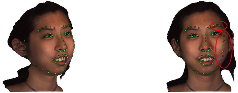
Automatic face alignment requires a large number of training examples of annotated images. Annotation is usually done using 2D images, where the annotator selects the locations of fiducial points around permanent facial features (e.g., brows and eyes). For frontal faces, reliable annotation can be achieved. As face orientation varies from frontal, however, annotated points lose correspondence. Pose variation results in self-occlusion that confounds landmark annotation. For example, consider the landmarks on the eyebrow and jawline. With increasing rotation and associated self-occlusion, annotations no longer correspond to the same landmarks on profile and frontal view images. See Figure 2 for an illustration of this problem. This issue can be alleviated by using 3D face-scans and annotating the 3D meshes themselves, instead of the 2D images.

Figure 2.

The 2D annotation of a profile-view image mapped on a frontal view face. Note, that certain landmarks (eyebrow, jawline) do not correspond to the same points on the two views because of the different head-poses and self-occlusions.

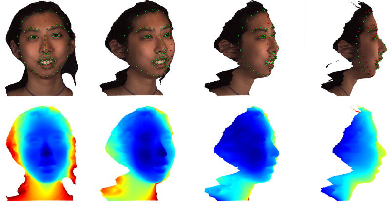
The 3D meshes were manually annotated with 77 landmarks, corresponding to facial fiducial points. This coarse set of landmarks had the same semantic meaning across subjects and expressions. Figure 3 shows the annotated and rotated meshes with the annotated landmarks and the corresponding depth maps. Since the annotation is 3D, we can identify the self-occluded landmarks from every pose.

Figure 3.

The 77 point annotation of the 3D mesh (top-left image), and profile views (30-60-90 degrees of yaw rotation). The color of the landmarks indicate the visibility from the given viewpoint (green – visible, red – occluded). The bottom row shows the corresponding depth images.

The time-consuming annotation process can be accelerated by using the semi-automatic approach of Baltrusaitis et al. [30].

2.4. Dense 3D Correspondence

While the coarse set of manually annotated landmarks has the same semantic meaning across subjects and expressions, to create a dense model that spans the data of multiple subjects requires establishing dense point-to-point correspondences among them [10, 31]. This means that the position of each vertex may vary in different samples, but its context label should remain the same. To establish dense correspondence, we used the Wave Kernel Signature (WKS) [32].

WKS is a novel shape feature descriptor. It is based on the Laplace–Beltrami operator [33] and carries a physical interpretation: it arises from studying the Schrödinger equation governing the dissipation of quantum mechanical particles on the geometric surface. The WKS enables accurate feature matching (see [32] for more details).

The number of vertices and their locations vary across the 3D face scans. To establish a reference shape, we used ordinary Procrustes analysis [34] with the 77 3D landmarks and registered each mesh to the same frame.

We then calculated a dense mean shape by uniformly subsampling the meshes down to 5000 vertices and calculating WKS descriptors for this reference shape as well.

We are interested in a model where we can easily control the level of detail of the 3D mesh. To build such a model, we employed a coarse-to-fine mesh refinement that resembles an adaptive $\sqrt{3}$-subdivision [35] scheme. We started from the reference shape and its triangulated 77-points mesh. Since this annotation corresponds to fiducial points and is not based on uniform sampling or surface complexity, applying the original $\sqrt{3}$-subdivision would result in unnecessary details around these landmarks. Therefore, in every step we apply the subdivision only on the triangle with the largest surface area and project the centroid back to the dense mesh. This procedure results in a tessellation, where the vertices are evenly distributed on the surface, follow the original geometry and the level of detail can be easily managed. After we tessellated the reference mesh, we identify the corresponding vertices from every mesh by finding the closest WKS match. See Figure 4 for an illustration of the method. We stopped the process at 1024 vertices. In Section 4.2 we give a more detailed explanation why we choose this level of detail. We used these 1024 vertices meshes to build our part-based linear model.

Figure 4.

Surface tessellation using the adaptive refinement scheme. The vertices are evenly distributed on the surface and they follow the original geometry.

2.5. Part-based model building

In Eq. (2) one can assume that the prior of the parameters follow a normal distribution with mean 0 and variance Λ at a parameter vector q: p(q) ∝ N(q;0, Λ) and can use Principal Component Analysis (PCA) to determine the d pieces of 3M dimensional basis vectors (Φ = [Φ₁;…; Φ_M] ∈ ℝ^3M×d). This approach has been used successfully in a broad range of face alignment techniques, such as Active Appearance Models [2] and 3D Morphable Models [10]. Although this procedure would result in a holistic shape model with a high compression rate, its components have a global reach and lack semantic meaning.

The deformations on the face can be categorized into two separate subsets: rigid (the shape of the face) and non-rigid (facial expressions) parts. We reformulate Eq. (2) to model these deformations separately:

$${\mathbf{x}}_i={\mathbf{x}}_i(\mathbf{p},\mathbf{r},\mathbf{s})=s\mathbf{R}({\overline{\mathbf{x}}}_i+{\mathbf{\Theta }}_i\mathbf{r}+{\mathbf{\Psi }}_i\mathbf{s})+\mathbf{t}(i=1,\dots ,M),$$ (3)

where the d pieces of 3M dimensional basis vectors (Θ = [Θ₁;…; Θ_M] ∈ ℝ^3M×d) describes the rigid, and the the e pieces of 3M dimensional basis vectors (Ψ = [Ψ₁;…; Ψ_M] ∈ ℝ^3M×e) describes the non-rigid deformations.

To build the rigid part, we selected neutral frames from each subjects and applied PCA to determine the basis vectors (Θ) and their mean (x̄). This provide us a holistic linear subspace, that describes the variation of the face shape only. Note that the neutral face is only required during the model building, it is not required for testing.

To build a linear subspace that describes the non-rigid deformations (Ψ) we follow the method of Tena et al [36]. The goal is to build a model that is composed of a collection of PCA part-models that are independently trained yet share soft boundaries. This model generalizes to unseen data better than the traditional holistic approach. To create the part-based-models, we group vertices that are highly correlated and form compact regions, since these regions will be better compressed by PCA. To find a data-driven segmentation of the facial expressions, we used all 6000 frames selected from the BU-4DFE and BP-4D-Spontaneous datasets. From each mesh, we subtracted the person’s own neutral face to remove all their personal variation from the data. Had we used the global mean (x̄) for the subtraction, some personal variation would have remained.

Our data D ∈ ℝ^6000×3072 consist of 6000 frames and 1024 3D vertices. We split D into three subsets D_x, D_y, D_z ∈ ℝ^6000×1024 each containing the corresponding spatial coordinate of the vertices. To describe the measurement of the correlation between vertices, the normalized correlation matrices are computed from D_x, D_y, D_z and then averaged into a global correlation matrix C. Vertices in the same region should also be close to each other on the face surface. Accordingly, we also compute the inter-vertex distance on the mesh as described in [36] for the isomap algorithm [37] to form a distance matrix G and normalized it to the [0, 1] scale. Both matrices are added into an affinity matrix A and spectral clustering wes performed on it using the method of Ng et al. [38].

In this study, we obtained 12 compact clusters instead of 13 as reported in [36]. A possible reason for this is that we lowered the 11 forehead landmarks from the manual annotation before calculating the dense mesh, resulting in a missing separate forehead region. These landmarks were on the border of the hair region, which was not estimated correctly by the imaging hardware in the dataset.

3. Model Fitting

In this section we describe the dense cascade regression and the 3D model fitting process.

3.1. Training dataset

Automatic face alignment requires a large number of training examples of annotated images. We used our 6000 annotated meshes and from each mesh we generated 63 different views in 20 degrees yaw rotation and 15 degrees pitch rotation increments (9 yaw and 7 pitch rotations in total). Resulting in the total number of 378,000 frames. For each view we calculated the corresponding rotated 3D landmarks and their 2D projections with self-occlusion information. Since the 3D meshes do not contain backgrounds, we included randomly selected non-face backgrounds in the final 2D images to increase the variety. These generated and annotated images were used to train a dense, cascade regression based method, that we detail in the next subsection.

3.2. Dense Cascade Regression

In this section we describe the general framework of dense cascade regression for face alignment. We build on the work of Xiong and De la Torre [7]. Given an image d ∈ ℝ^a×1 of a pixels, d(y) ∈ ℝ^b×1 indexes b landmarks in the image. Let h to be a feature extraction function (e.g. HOG, SIFT or binary features) and h(d(y)) ∈ ℝ^Fḃ×1 in the case of extracting features of length F. During training we will assume that the ground truth location of the b landmarks are known. We refer to them as y_⋆.

We used a face detector on the training images to provide an initial configuration of the landmarks (y₀), which correspond to the frontal projection of the 3D reference face built in Section 2.4.

In this framework, face alignment can be framed as minimizing the following function over (Δy):

$$f({\mathbf{y}}_0+\mathrm{\Delta }\mathbf{y})={\Vert \mathbf{h}(\mathbf{d}({\mathbf{y}}_0+\mathrm{\Delta }\mathbf{y}))-{\beta }_{\star }\Vert }_2^2$$ (4)

where β_⋆ = h(d(y_⋆)) represents the feature values in the ground truth landmarks.

The feature extraction function (h) can be highly non-linear and minimizing eq. (4) would require numerical approximations, which are computational expensive. Instead we learn a series of linear regressor matrices (R_i), such that it produces a sequence of updates starting from y₀ that converges to y_⋆ in the training data:

$$\mathrm{\Delta }{\mathbf{y}}_i={\mathbf{R}}_{i-1}{\beta }_{i-1}+{\mathbf{b}}_{i-1}$$ (5)

$${\mathbf{y}}_i={\mathbf{y}}_{i-1}+\mathrm{\Delta }{\mathbf{y}}_i\to {\mathbf{y}}_{\star }$$ (6)

In our case, the annotation y consist of the projected 2D locations of the 3D landmarks and their corresponding visibility information:

$$\mathbf{y}=[x_1;y_1;{\nu }_1;\dots ;x_M;y_M;{\nu }_M],$$ (7)

where ν_i ∈ [0, 1] indicates if the landmark is visible (ν_i = 1) or not (ν_i = 0).

3.3. 3D Model Fitting

The dense cascade regressor defined in the previous section provides projected 2D locations of the 3D landmarks. To reconstruct the 3D shape from the 2D shape (z) we need to minimize the reconstruction error using eq. (3):

$$\underset{\mathbf{p},\mathbf{r},\mathbf{s}}{\text{arg min}}\sum _{i=1}^M{\Vert {\mathbf{\text{Px}}}_i(\mathbf{p},\mathbf{r},\mathbf{s})-{\mathbf{z}}_i\Vert }_2^2$$ (8)

Here P denotes the projection matrix to 2D, and z is the target 2D shape. An iterative method can be used to register 3D model on the 2D landmarks [13]. The algorithm iteratively refines the 3D shape and 3D pose until convergence, and estimates the rigid (p = {s, α, β, γ, t}) and non-rigid transformations (r and s).

This equation assumes that there is a semantic correspondence between the 2D and 3D landmarks. The lack of correspondence requires a correction step [25], usually in a form of a selection matrix [39], that selects the right 3D landmarks corresponding to the 2D ones.

In our case the semantic correspondence has been established during model building time: the landmarks provided by the cascade regressor are 2D projections of the 3D landmarks. Furthermore, the cascade regressor estimates the visibility of landmarks. We can incorporate this information in eq. (8), by constraining the process to the visible landmarks:

$$\underset{\mathbf{p},\mathbf{r},\mathbf{s}}{\text{arg min}}\sum _{i\in \mathit{\xi }}{\Vert {\mathbf{\text{Px}}}_i(\mathbf{p},\mathbf{r},\mathbf{s})-{\mathbf{z}}_i\Vert }_2^2$$ (9)

where ξ = {j|ν_j = 1} denotes the subset of landmark-indices that are visible (see eq. (7)).

Applying eq. (9) on a single image frame from a monocular camera has a drawback of simply ”hallucinating” a 3D representation from 2D. From a single viewpoint there are multiple solutions that satisfy eq. (9). To avoid the problem of single frame 2D–3D hallucination we apply the method simultaneously across multiple image-frames.

Let us assume that we have access to time-synchronized 2D measurements (z⁽¹⁾, …, z^(C)) from a multi-view setup consisting of C cameras. The exact camera locations and camera calibration matrices are unknown. In this case all C measurements represent the same 3D face, but from a different point of view. We can extend eq. (9) to this scenario by constraining the reconstruction to all the measurements:

$$\underset{\begin{array}{c}\hfill {\mathbf{p}}^{(1)},\dots ,{\mathbf{p}}^{(C)},\hfill \\ \hfill \mathbf{r},\mathbf{s}\hfill \end{array}}{\text{arg min}}\sum _{k=1}^C\sum _{i\in {\mathit{\xi }}^{(k)}}{\Vert {\mathbf{\text{Px}}}_i({\mathbf{p}}^{(k)},\mathbf{r},\mathbf{s})-{\mathbf{z}}_i^{(k)}\Vert }_2^2$$ (10)

where superscripts (k) denote the k^th measurement, with a visibility set of ξ^(k). Note that in this case both the holistic rigid (r) and the part-based non-rigid (s) deformations are the same for all measurements, since we are observing the same face, but from different views.

In a more common, everyday scenario, such as monocular videos, we don’t have access to time-synchronized multiple spatial measurements. In this case we can still assume that the rigid structure of the face (parameter r) will have little variation, only the expressions will change (parameter s). To handle this situation, we relax eq. (10) and solve it in the temporal domain. Let us assume that we have access to T temporal 2D measurements from a video sequence. In the first step we estimate the rigid deformation parameters:

$$\underset{{\mathbf{r}}_{\tau }}{\text{arg min}}\sum _{t\in \mathit{\tau }}\sum _{i\in {\mathit{\xi }}^{(t)}}{\Vert {\mathbf{\text{Px}}}_i({\mathbf{p}}^{(t)},{\mathbf{r}}_{\mathit{\tau }},\mathbf{0})-{\mathbf{z}}_i^{(t)}\Vert }_2^2$$ (11)

where τ = {z^(t)|t = 1, …, T} denotes the set of temporal measurements, and r_τ denotes the rigid deformation parameters estimated from τ. Note that in this step the non-rigid deformation parameters are set to 0 (s = 0).

In the second step, we estimate the rigid deformation parameters at an arbitrary time step t ∈ [1, …, T]:

$$\underset{{\mathbf{p}}^{(t)},{\mathbf{s}}^{(t)}}{\text{arg min}}\sum _{i\in {\mathit{\xi }}^{(t)}}{\Vert {\mathbf{\text{Px}}}_i({\mathbf{p}}^{(t)},{\mathbf{r}}_{\mathit{\tau }},{\mathbf{s}}^{(t)})-{\mathbf{z}}_i^{(t)}\Vert }_2^2$$ (12)

4. Experiments

We conducted a battery of experiments to evaluate the precision of 3D reconstruction and extensions to multi-view reconstruction. Studies concern (i) feature spaces, (ii) optimal model density, (iii) number of measurements in single- and (iv) multi-view scenario, (v) temporal integration and (vi) the performance of 3D head pose estimation under various illumination conditions.

4.1. Feature space for the cascade regression

In this experiment we evaluated SIFT [40] and localized binary features [41] for training the regression cascades. For each shape in the training set we generated samples using the Monte-Carlo procedure by perturbing the model parameters of the ground truth shapes. SIFT and binary descriptors were computed on 32×32 local patches around the landmarks. In the case of binary features, we used a low-rank PCA [42] to learn a compressed representation of the patches. We kept 128 dimensions in the process for each landmark.

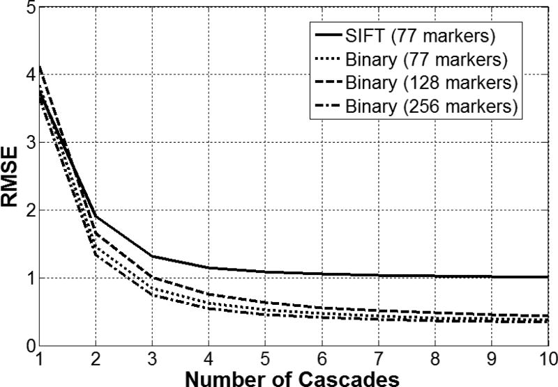
We used a five-fold cross-validation to calculate the landmark estimation precision, measured by the root mean squared error of landmark displacements. We found that binary feature representation learned from the data outperformed hand crafted SIFT features (see Figure 5).

Figure 5.

Landmark RMSE as a function of cascades. 1 RMSE unit correspond to 1 pixel error in all landmarks. The inter-ocular distance was normalized to 100 pixels.

Binary features are a magnitude faster than SIFT, allowing more landmarks to be measured. We varied the number of observed vertices using binary features from 77 to 256. The effect in terms of RMSE is noticeable, but not significant. After 6–7 iterations, we observed a plateauing effect in the RMSE.

We also investigated the effect of different illumination conditions by varying the level of ambient light and adding directional light. The method was robust to these perturbations. Binary features, like SIFT features, were insensitive to photometric variation in the input images.

4.2. Optimal density of the model

In this experiment, we studied the reconstruction precision of the 3D model with different level of details. We identified a minimum set of vertices that are required in the model to reconstruct the 3D geometry of the face with high precision.

First we registered and tessellated the ground truth meshes according to Section 2.4.

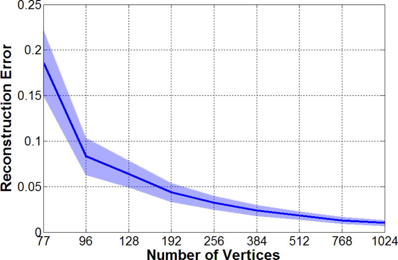
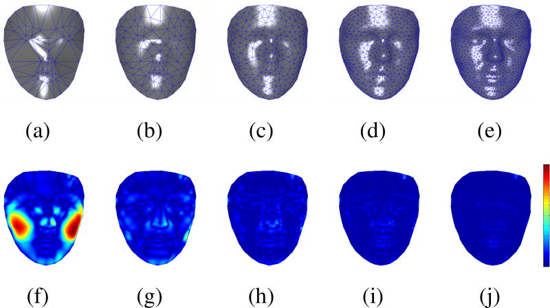
We rendered the reconstructed 3D shapes and their corresponding depth maps. Accurate depth maps of the ground truth meshes are also computed for comparison. The differences between the two depth maps are computed and they were summed up within the area bounded by the face outline. The final score was normalized to the area of the original face. This normalized score served as the measure for evaluating the reconstruction precision (Reconstruction Error). Since the tessellation is done in an adaptive manner, this provides an easy way to vary the number of vertices. We varied this number between 77 and 1024 on a logarithmic scale

The results are summarized in Figure 6. The original data consist of more than 30,000 vertices. The figure shows that we can precisely approximate them using around 1,000 vertices. We suspended refinement at M = 1024 vertices.

Figure 6.

The reconstruction error as a function of vertices. The solid line (shaded region) shows the mean error (standard deviation).

Figure 7 shows the different levels of detail and the corresponding absolute depth map differences comparing with the ground truth mesh.

Figure 7.

Visualizing the reconstructed 3D meshes with different levels of detail. (a)–(e) Meshes consisting of 77, 128, 256, 512 and 1024 vertices, respectively. (f)–(j) The corresponding absolute depth map differences comparing with the ground truth mesh.

4.3. Number of measurements and iterations for fitting

Two important questions are the number of vertices to measure and the number of iteration steps needed during model fitting (Section 3.3). We expected that a much smaller subset of vertices would be sufficient for the fitting given the inherent 3D surface constraints.

To test this hypothesis, we kept the total number of vertices in the model fixed (M = 1024) and varied the number of vertices (M_Obs) from 77 to 1024 on a logarithmic scale. For selecting the observed vertices we used the same scheme as before: we used the first 77, 128, 256, etc. vertices from the refining process. This way we add more detail to the mesh and more constraint to the model fitting.

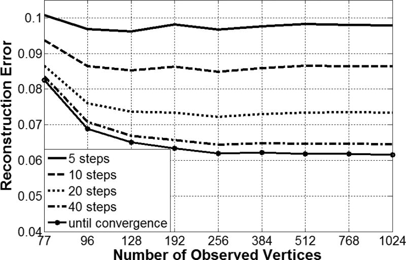
Another parameter is the number of iterations during the model fitting. We varied the number of iterations between 5 and 40 on a logarithmic scale. Figure 8 shows reconstruction error as a function of observed vertices and the number of iteration steps.

Figure 8.

The reconstruction error as a function of observed vertices M_Obs and the number of iteration steps using a single measurement.

The figure shows that there is no further performance gain measuring more than 128 vertices. The size of the cascade regressor matrices and the fitting speed depends on the number of observed vertices. As we see, we can keep this number low without the loss of precision.

The number of iterations during the fitting had a significant effect on the reconstruction error. Increasing the number of iterations steps has no effect on the model size.

4.4. Multi-view measurements

Up until now, we used only a single frame to locate the landmarks and fit the 3D model. In this experiment, we investigated the performance gain when we have access to multiple measurements for each time-step.

Let us assume that we have a time-synchronized multi-camera setup that provides two frames at every time-step, but the exact camera locations and the camera calibration matrices are unknown.

We fixed the total number of vertices in the model (M = 1024) and varied the number of observed vertices (M_Obs) between 77 and 512 on a logarithmic scale. For selecting the observed vertices, we used the same scheme as before: we used the first 77, 128, 256, etc. vertices from the refining process. This way we add more detail to the mesh and more constraint to the model fitting.

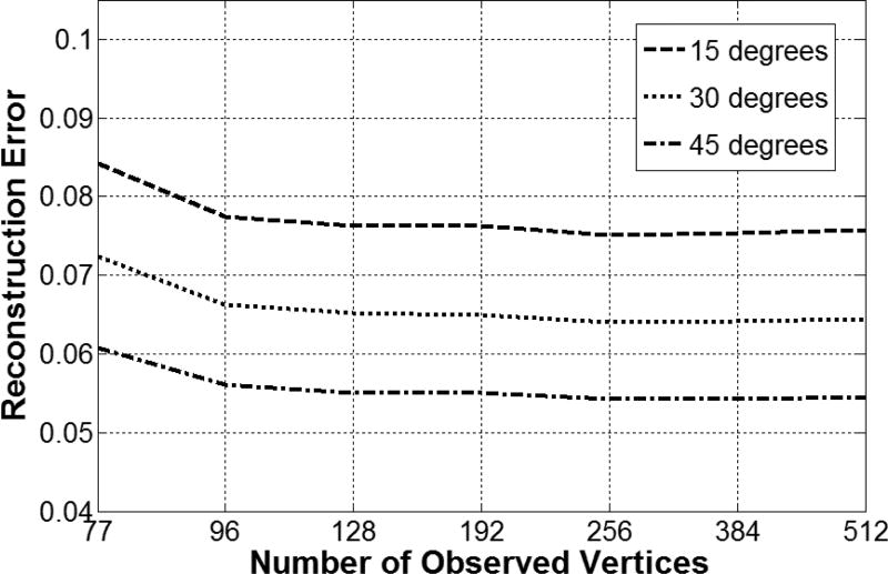
Figure 9 shows the reconstruction error as a function of observed vertices M_Obs using two synchronized cameras that are separated by 15, 30 and 45 degrees of yaw rotations apart. The number of iterations was fixed in 10 steps. The figure shows that larger viewpoint-angles yielded lower reconstruction error.

Figure 9.

The reconstruction error as a function of observed vertices M_Obs using two synchronized cameras that are separated by 15, 30 and 45 degrees of yaw rotations apart.

4.5. Temporal Integration

In a everyday scenario, such as monocular videos, we don’t have access to time-synchronized multiple spatial measurements. In this case we can still assume that the rigid structure of the face (parameter r) will have little variation, only the expressions will change (parameter s). To test this hypothesis, we conducted an experiment with different number of temporal measurements (τ).

In an offline scenario, where all the frames are available during testing time, r_τ can be pre-calculated for each subject. After this, the rigid parameters (p) and the non-rigid deformation parameters (s) can be computed for each frame. In an online case, one can add new samples to τ as they become available and can recalculate r_τ on the fly.

In both cases the size of τ can be significantly large, however not every sample is important equally for the estimation of r_τ. A small sample-set that covers a wide head-pose range will yield to smaller reconstruction error. One could include a new sample in τ if its orientation is significantly different from the previous ones.

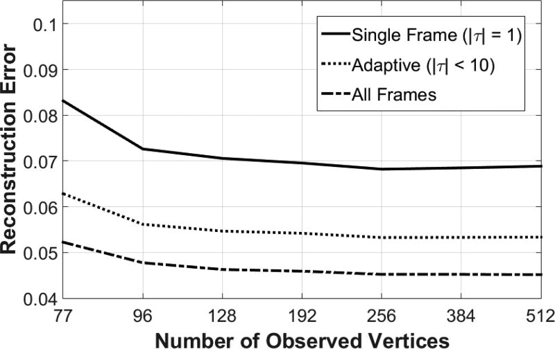
We used 5 short video sequences from the BP4D-Spontaneous dataset with moderate head movements and tested three different cases: (i) single frame reconstruction, (ii) adaptive number of temporal measurements and (iii) using all the available frames. In the adaptive case we maximized the number temporal measurements at 10, and we only included a new measurement to τ if the mean angular difference of the yaw and pitch angles was higher than 10 degrees than the previously included measurements. Every video sequence started with and empty τ set.

Figure 10 shows the reconstruction error as a function of observed vertices M_Obs using the three different strategies. The number of iterations was fixed in 10 steps. The figure shows that using all the available frames yielded the lowest reconstruction error. The adaptive strategy achieved precise reconstruction using significantly less data.

Figure 10.

The reconstruction error as a function of observed vertices M_Obs using three different temporal integration strategies: (i) single-frame reconstruction, (ii) adaptive temporal measurements and (iii) using all the available frames.

4.6. Head-pose estimation using Dense Models

In this experiment we evaluate the performance of the proposed method for head tracking using real faces from the Boston University (BU) head tracking database [43].

4.6.1. Boston University Head Tracking Dataset

We used the Boston University Head Tracking dataset [43] to evaluate the performance of the proposed method for 3D head-pose estimation. The database contains short video sequences of different subjects with uniform (45 videos) and varying (27 videos) illuminations at a resolution of 320 × 240 pixels. Subjects were asked to perform various head movements, including translation and rotation, without distinctive facial expressions.

The dataset also contains ground truth information of the head position and orientation, collected by the Flock of Birds magnetic tracker attached on the subject’s head.

4.6.2. Uniform Illumination Subset

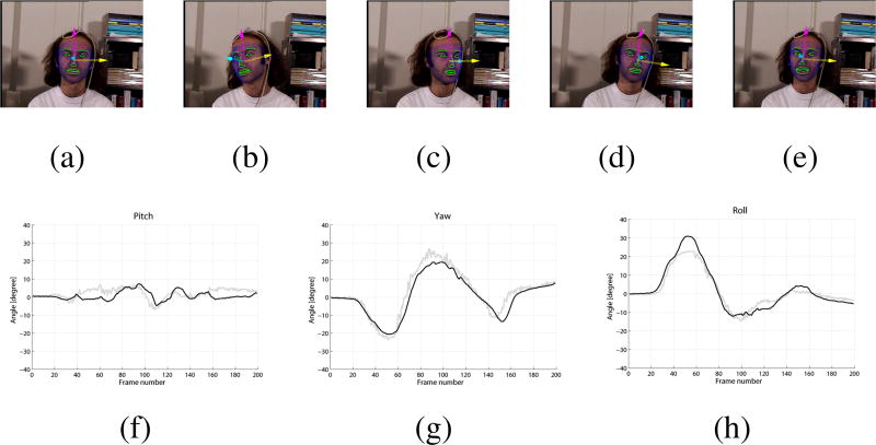
First, we used the uniform illumination subset (45 sequences) of the BU database and compared the estimated head pose to the ground truth provided in the dataset. Figure 11 shows an example tracking sequence. The mean absolute angular error of the head pose estimation is shown in Table 1 in comparison with results from different sources. The accuracies of Cascia et al. [43] and Xiao et al. [44] are taken from [51].

Figure 11.

An example tracking sequence from the uniform illumination subset of the database. (a)–(e): Tracked frames number 0, 40, 80, 120 and 160. (f)–(h): Pitch/Yaw/Roll estimation. In each graph, the black curve depicts the estimated value and the gray curve depicts the ground truth.

Table 1.

Comparison of different head tracking results on the Boston University dataset. The numbers represent the mean absolute angular error of the head pose estimation in degrees. The accuracies of Cascia et al. [43] and Xiao et al. [44] are taken from [51].

Method	Pitch	Yaw	Roll	Mean
La Cascia et al. (CT) [43]	6.1	3.3	9.8	6.4
Xiao et al. (CT) [44]	3.2	3.8	1.4	2.8
Asteriadis et al. (DVF) [45]	3.82	4.56	-	4.19
Kumano et al. (PF) [46]	4.2	7.1	2.9	4.73
Sung et al. (AAM+CT) [47]	5.6	5.4	3.1	4.7
Valenti et al. (CT) [48]	5.26	6.10	3.00	4.79
An & Chung (ET) [49]	7.22	5.33	3.22	5.26
Saragih et al. (CLM) [50]	4.5	5.2	2.6	4.1
Vincente et al. (SDM) [39]	6.2	4.3	3.2	4.6
This work (Dense 3D)	2.66	3.93	2.41	3.00

Acronyms: CT - Cylindrical Tracker, DVF - Distance Vector Field, PF - Particle Filter, AAM - Active Appearance Model, ET - Ellipsoidal Tracker, CLM - Constrained Local Model, SDM - Supervised Descent Method.

4.6.3. Varying Illumination Subset

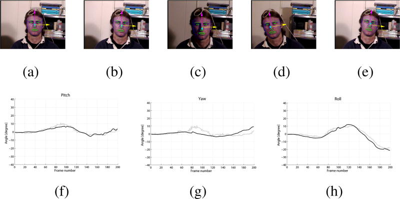
In the second part of the experiment we used the varying illumination subset (27 sequences) to evaluate the effect of the changing lighting conditions on the pose estimation. Figure 12 shows an example tracking sequence from the varying illumination subset. The mean absolute angular error of the Pitch, Yaw and Roll angle estimation is 2.72°, 4.87° and 2.24° respectively.

Figure 12.

An example tracking sequence from the varying illumination subset of the database. (a)–(e): Tracked frames number 0, 40, 80, 120 and 160. (f)–(h): Pitch/Yaw/Roll estimation. In each graph, the black curve depicts the estimated value and the gray curve depicts the ground truth.

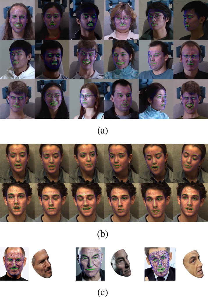
The results demonstrated that the proposed method is able to estimate head pose with high accuracy, even under varying lighting conditions. The method achieved the best result for Pitch angle estimation, and the second best result overall. We note that the Yaw and Roll angle estimations are slightly lower than the tracker proposed in [44], however our method is able to simultaneously estimate the head pose and reconstruct a dense 3D mesh of the face. Further qualitative results are presented in Figure 13.

Figure 13.

Examples from (a) Multi-PIE with various illuminations and head poses, (b) RU-FACS tracking sequences and (c) celebrities with profile view renders using the high-resolution 3D shape. The contours of key facial parts are highlighted in green for display purpose.

5. Discussion and Conclusions

Faces move, yet most approaches to face alignment use a 2D representation that effectively assumes the face is planar. For frontal or nearly frontal views, this fiction works reasonably well. As rotation from frontal view increases, however, approaches that assume 2D representation begin to fail. Action unit detection becomes less accurate after about 15 to 20 degrees rotation from frontal [52] and expression transfer to a near-photo-realistic avatar fails when the source face rotates beyond this range [53]. Several previous solutions to this problem have been proposed for real-time use. Kanaujia and Metaxas proposed training 2D models for face rotations from 0 through 90 degrees [54]. While this is a reasonable solution, it requires large amounts of multiview images sampled across the range of interest. Another possible solution is to ”hal-lucinate” 3D information from a single image-frame [2]. Recently, Tulyakov and Sebe [55] achieved good 3D reconstruction by augmenting 2D information with corresponding 3D factors in the regression procedure. With this approach, facial landmarks can be only sparsely sampled, and it’s not well suited for image synthesis. Motion capture can provide dense tracking and alignment, but requires placement of hundreds of reflective markers for dense tracking, which is time intensive and may inhibit movement spontaneity, and necessitate bright lights, which can further contribute to reactivity effects. Structured light displays similarly require high illumination and attendant increases in electrical power and computational cost.

We developed a method that has two innovations. First, we proposed the novel employment of a dense (over 1000 vertex) compact spatio-temporal 3D face model. While it is easy to obtain individual dense 3D face scans through 3D cameras or scanners, it is non-trivial to have an ensemble of such scans in semantic correspondence in space and time. The compactness of this dense model is essential in terms of fitting and energy efficiency performance. Second, we propose a regression based 3D fitting method that is simultaneously applied across multiple image-frames to avoid the problem of single frame 2D–3D hallucination.

We studied hand crafted SIFT [40] and localized binary features [41] for training the regression cascades. We evaluated the landmark estimation precision measured by the root mean squared error of their displacements. We found that the binary representation learned from the data outperformed the generic SIFT features. In turn, we engaged in studies using the binary features, which are a magnitude faster than SIFT, allowing use of greater number of landmarks while still achieves real-time performance.

We used a variety of evaluations to determine the minimum set of vertices to reconstruct the 3D geometry of the face with high fidelity. Ground truth 3D scans consisted of more than 30,000 vertices. We found that we could precisely approximate this level of detail using around 1000 vertices. Two important questions required further considerations: the optimal number of vertices to measure and the number of iterations required during model fitting. We anticipated that a smaller subset of vertices would be sufficient due to the inherent 3D surface constraints of the face. We found that information gain peaked at about 128 vertices. The number of iterations during the fitting had a significant effect on the reconstruction error.

A common strategy to estimate the approximate 3D structure and camera position of the 2D facial landmarks is to minimize the error between the 2D landmarks and the 2D projection of the 3D deformable model. Although well understood [2], and successfully employed in conjunction with numerous 2D facial landmark alignment systems the approach simply ”hallucinates” the 3D structure and the camera position for each frame independently. To circumvent this issue, we investigated the performance gain when we have access to multiple measurements for each time-step. We used a time-synchronized multi-view setup that provided two frames at each time-step. The camera locations and calibration matrices were unknown. Larger viewpoint-angles yielded lower reconstruction error and fewer iterations are required for the same level of precision as in the single frame case.

We studied the robustness of the proposed method for 3D head-pose estimation under various conditions. We tracked all the subjects from the Boston University (BU) head tracking database [43] and compared the results to nine state-of-the-art methods. We found that our method was able to estimate head pose with high accuracy, even under changing lighting conditions. For pitch angle estimation, the proposed method was strong winner; overall, the proposed method ranked second only to the cylindrical tracker from Xiao et al. [44]. Xiao’s method, of course, only tracks the head orientation. Ours reconstructs a dense 3D mesh of the face as well.

The proposed method is computationally efficient due to two main factors. First, we employ a sparse sampling strategy at feature level. An obvious strength to the dense sampling strategy is the amount of explicit and implicit ordinal information it encodes. With a sparse comparison strategy one encodes less ordinal information, but is computationally more efficient since one requires less comparisons and the resulting feature vector is smaller. Second, classical methods, such as 3D Morphable Models, require the computationally expensive task of inverting a large generative model during the alignment process. They linearize the system around the current estimate of the parameters, perform a constrained/projected gradient step then update the estimate, iterating this procedure until convergence. In our case this process is discrete and dependent only on the current iteration. The act of alignment also becomes extremely efficient as the only cost of sampling the gradient step is a memory lookup and matrix multiplications. Furthermore, the number of lookups is fixed to the number of iterations. Our MATLAB implementation runs at 50 fps using a single core of an i7 processor.

In summary, we found that high-precision, dense 3D registration and reconstruction can be achieved from 2D video in real-time. The method can be of high value in real-time facial expression analysis and avatar animation.

References

- 1.Cootes T, Edwards G, Taylor C. Active appearance models, Pattern Analysis and Machine Intelligence. IEEE Transactions on. 2001;23(6):681–685. doi: 10.1109/34.927467. [DOI] [Google Scholar]
- 2.Matthews I, Baker S. Active appearance models revisited. International Journal of Computer Vision. 2004;60(2):135–164. [Google Scholar]
- 3.Cristinacce D, Cootes T. Automatic feature localisation with constrained local models. Pattern Recogn. 2008;41(10):3054–3067. doi: 10.1016/j.patcog.2008.01.024. [DOI] [Google Scholar]
- 4.Saragih JM, Lucey S, Cohn JF. Deformable model fitting by regularized landmark mean-shift. International Journal of Computer Vision. 2011;91(2):200–215. doi: 10.1007/s11263-010-0380-4. [DOI] [Google Scholar]
- 5.Dollar P, Welinder P, Perona P. Cascaded pose regression; Computer Vision and Pattern Recognition (CVPR), 2010 IEEE Conference on; 2010. pp. 1078–1085. [DOI] [Google Scholar]
- 6.Cao X, Wei Y, Wen F, Sun J. Face alignment by explicit shape regression; Computer Vision and Pattern Recognition (CVPR), 2012 IEEE Conference on; 2012. pp. 2887–2894. [DOI] [Google Scholar]
- 7.Xiong X, De la Torre F. Supervised descent method and its applications to face alignment; Computer Vision and Pattern Recognition (CVPR), 2013 IEEE Conference on; 2013. pp. 532–539. [DOI] [Google Scholar]
- 8.Burgos-Artizzu X, Perona P, Dollar P. Robust face landmark estimation under occlusion; Computer Vision (ICCV), 2013 IEEE International Conference on; 2013. pp. 1513–1520. [DOI] [Google Scholar]
- 9.Ren S, Cao X, Wei Y, Sun J. Face alignment at 3000 fps via regressing local binary features; Computer Vision and Pattern Recognition (CVPR), 2014 IEEE Conference on; 2014. pp. 1685–1692. [DOI] [Google Scholar]
- 10.Blanz V, Vetter T. Proceedings of the 26th Annual Conference on Computer Graphics and Interactive Techniques, SIGGRAPH ’99. ACM Press/Addison-Wesley Publishing Co.; New York, NY, USA: 1999. A morphable model for the synthesis of 3d faces; pp. 187–194. [DOI] [Google Scholar]
- 11.Dimitrijevic M, Ilic S, Fua P. Accurate face models from uncalibrated and ill-lit video sequences. Computer Vision and Pattern Recognition, 2004. CVPR 2004, Proceedings of the 2004 IEEE Computer Society Conference on. 2004;2:II–1034–II–1041. doi: 10.1109/CVPR.2004.1315278. Vol.2. [DOI] [Google Scholar]
- 12.Zhang Z, Liu Z, Adler D, Cohen MF, Hanson E, Shan Y. Robust and rapid generation of animated faces from video images: A model-based modeling approach. Int. J. Comput. Vision. 2004;58(2):93–119. doi: 10.1023/B:VISI.0000015915.50080.85. [DOI] [Google Scholar]
- 13.Gu L, Kanade T. 3d alignment of face in a single image. Computer Vision and Pattern Recognition, 2006 IEEE Computer Society Conference on. 2006;1:1305–1312. doi: 10.1109/CVPR.2006.11. [DOI] [Google Scholar]
- 14.Kemelmacher-Shlizerman I, Basri R. 3d face reconstruction from a single image using a single reference face shape, Pattern Analysis and Machine Intelligence. 28 IEEE Transactions on. 2011;33(2):394–405. doi: 10.1109/TPAMI.2010. [DOI] [PubMed] [Google Scholar]
- 15.Hassner T. Viewing real-world faces in 3d; Computer Vision (ICCV), 2013 IEEE International Conference on; 2013. pp. 3607–3614. [DOI] [Google Scholar]
- 16.Suwajanakorn S, Kemelmacher-Shlizerman I, Seitz S. Total moving face reconstruction. In: Fleet D, Pajdla T, Schiele B, Tuytelaars T, editors. Computer Vision, ECCV 2014, Vol. 8692 of Lecture Notes in Computer Science. Springer International Publishing; 2014. pp. 796–812. [DOI] [Google Scholar]
- 17.Dantone M, Gall J, Fanelli G, Gool LV. Real-time facial feature detection using conditional regression forests. CVPR. 2012 [Google Scholar]
- 18.Sun Y, Wang X, Tang X. Deep convolutional network cascade for facial point detection; Computer Vision and Pattern Recognition (CVPR), 2013 IEEE Conference on; 2013. pp. 3476–3483. [DOI] [Google Scholar]
- 19.Valstar M, Martinez B, Binefa X, Pantic M. Facial point detection using boosted regression and graph models; Computer Vision and Pattern Recognition (CVPR), 2010 IEEE Conference on; 2010. pp. 2729–2736. [DOI] [Google Scholar]
- 20.Martinez B, Valstar M, Binefa X, Pantic M. Local evidence aggregation for regression-based facial point detection, Pattern Analysis and Machine Intelligence. IEEE Transactions on. 2013;35(5):1149–1163. doi: 10.1109/TPAMI.2012.205. [DOI] [PubMed] [Google Scholar]
- 21.Zhang J, Shan S, Kan M, Chen X. Coarse-to-fine auto-encoder networks (cfan) for real-time face alignment. In: Fleet D, Pajdla T, Schiele B, Tuytelaars T, editors. Computer Vision, ECCV 2014, Vol. 8690 of Lecture Notes in Computer Science. Springer International Publishing; 2014. pp. 1–16. [DOI] [Google Scholar]
- 22.Kazemi V, Sullivan J. One millisecond face alignment with an ensemble of regression trees; Computer Vision and Pattern Recognition (CVPR), 2014 IEEE Conference on; 2014. pp. 1867–1874. [DOI] [Google Scholar]
- 23.Asthana A, Zafeiriou S, Cheng S, Pantic M. Incremental face alignment in the wild; Computer Vision and Pattern Recognition (CVPR), 2014 IEEE Conference on; 2014. pp. 1859–1866. [DOI] [Google Scholar]
- 24.Cao C, Weng Y, Lin S, Zhou K. 3d shape regression for real-time facial animation. ACM Trans. Graph. 2013;32(4):41, 1–41, 10. doi: 10.1145/2461912.2462012. [DOI] [Google Scholar]
- 25.Cao C, Hou Q, Zhou K. Displaced dynamic expression regression for real-time facial tracking and animation. ACM Trans. Graph. 2014;33(4):43, 1–43, 10. doi: 10.1145/2601097.2601204. [DOI] [Google Scholar]
- 26.Yin L, Chen X, Sun Y, Worm T, Reale M. A high-resolution 3d dynamic facial expression database; Automatic Face Gesture Recognition, 2008. FG ’08. 8th IEEE International Conference on; 2008. pp. 1–6. [Google Scholar]
- 27.Zhang X, Yin L, Cohn JF, Canavan S, Reale M, Horowitz A, Liu P, Girard JM. Bp4d-spontaneous: a high-resolution spontaneous 3d dynamic facial expression database. Image and Vision Computing. 2014;32(10):692–706. best of Automatic Face and Gesture Recognition 2013. [Google Scholar]
- 28.Dimensional Imaging Ltd. DI3D. http://www.di3d.com.
- 29.Ekman P, Friesen W, Hager J. Facial Action Coding System (FACS): Manual. Salt Lake City (USA): A Human Face; 2002. [Google Scholar]
- 30.Baltrusaitis T, Robinson P, Morency L. Computer Vision and Pattern Recognition (CVPR), 2012 IEEE Conference on. IEEE; 2012. 3d constrained local model for rigid and non-rigid facial tracking; pp. 2610–2617. [Google Scholar]
- 31.Allen B, Curless B, Popović Z. The space of human body shapes: Reconstruction and parameterization from range scans. ACM Trans. Graph. 2003;22(3):587–594. doi: 10.1145/882262.882311. [DOI] [Google Scholar]
- 32.Aubry M, Schlickewei U, Cremers D. The wave kernel signature: A quantum mechanical approach to shape analysis; Computer Vision Workshops (ICCV Workshops), 2011 IEEE International Conference on; 2011. pp. 1626–1633. [DOI] [Google Scholar]
- 33.Levy B. Laplace-beltrami eigenfunctions towards an algorithm that ”understands” geometry; Shape Modeling and Applications, 2006. SMI 2006. IEEE International Conference on; 2006. pp. 13–13. [DOI] [Google Scholar]
- 34.Dryden KVMIL. Statistical Shape Analysis. John Wiley & Sons; 1998. [Google Scholar]
- 35.Kobbelt L. Proceedings of the 27th Annual Conference on Computer Graphics and Interactive Techniques, SIGGRAPH ’00. ACM Press/Addison-Wesley Publishing Co.; New York, NY, USA: 2000. Sqrt(3)-subdivision; pp. 103–112. [DOI] [Google Scholar]
- 36.Tena JR, De la Torre F, Matthews I. ACM SIGGRAPH 2011 Papers, SIGGRAPH ’11. Vol. 76. ACM; New York, NY, USA: 2011. Interactive region-based linear 3d face models; pp. 1–76.pp. 10 [DOI] [Google Scholar]
- 37.Tenenbaum JB, De Silva V, Langfold JC. A global geometric framework for nonlinear dimensionality reduction. Science. 2000;290(5500):2319–2323. doi: 10.1126/science.290.5500.2319. [DOI] [PubMed] [Google Scholar]
- 38.Ng AY, Jordan MI, Weiss Y. ADVANCES IN NEURAL INFORMATION PROCESSING SYSTEMS. MIT Press; 2001. On spectral clustering: Analysis and an algorithm; pp. 849–856. [Google Scholar]
- 39.Vicente F, Huang Z, Xiong X, De la Torre F, Zhang W, Levi D. Driver gaze tracking and eyes off the road detection system [Google Scholar]
- 40.Lowe DG. Distinctive image features from scale-invariant keypoints. Int. J. Comput. Vision. 2004;60(2):91–110. doi: 10.1023/B:VISI.0000029664.99615.94. [DOI] [Google Scholar]
- 41.Calonder M, Lepetit V, Ozuysal M, Trzcinski T, Strecha C, Fua P. Brief: Computing a local binary descriptor very fast, Pattern Analysis and Machine Intelligence. IEEE Transactions on. 2012;34(7):1281–1298. doi: 10.1109/TPAMI.2011.222. [DOI] [PubMed] [Google Scholar]
- 42.Halko N, Martinsson P, Tropp J. Finding structure with randomness: Probabilistic algorithms for constructing approximate matrix decompositions. SIAM Review. 2011;53(2):217–288. doi: 10.1137/090771806. [DOI] [Google Scholar]
- 43.La Cascia M, Sclaroff S, Athitsos V. Fast, reliable head tracking under varying illumination: An approach based on registration of texture-mapped 3d models, Pattern Analysis and Machine Intelligence. IEEE Transactions on. 2000;22(4):322–336. [Google Scholar]
- 44.Xiao J, Moriyama T, Kanade T, Cohn JF. Robust full-motion recovery of head by dynamic templates and re-registration techniques. International Journal of Imaging Systems and Technology. 2003;13(1):85–94. doi: 10.1002/ima.10048. [DOI] [PMC free article] [PubMed] [Google Scholar]
- 45.Asteriadis S, Soufleros D, Karpouzis K, Kollias S. Proceedings of the International Workshop on Affective-Aware Virtual Agents and Social Robots. ACM; 2009. A natural head pose and eye gaze dataset; p. 1. [Google Scholar]
- 46.Kumano S, Otsuka K, Yamato J, Maeda E, Sato Y. Pose-invariant facial expression recognition using variable-intensity templates. International journal of computer vision. 2009;83(2):178–194. [Google Scholar]
- 47.Sung J, Kanade T, Kim D. Pose robust face tracking by combining active appearance models and cylinder head models. International Journal of Computer Vision. 2008;80(2):260–274. [Google Scholar]
- 48.Valenti R, Sebe N, Gevers T. Combining head pose and eye location information for gaze estimation, Image Processing. IEEE Transactions on. 2012;21(2):802–815. doi: 10.1109/TIP.2011.2162740. [DOI] [PubMed] [Google Scholar]
- 49.An KH, Chung MJ. Intelligent Robots and Systems, 2008. IROS 2008. IEEE/RSJ International Conference on. IEEE; 2008. 3d head tracking and pose-robust 2d texture map-based face recognition using a simple ellipsoid model; pp. 307–312. [Google Scholar]
- 50.Saragih JM, Lucey S, Cohn JF. Deformable model fitting by regularized landmark mean-shift. International Journal of Computer Vision. 2011;91(2):200–215. [Google Scholar]
- 51.Murphy-Chutorian E, Trivedi MM. Head pose estimation in computer vision: A survey, Pattern Analysis and Machine Intelligence. IEEE Transactions on. 2009;31(4):607–626. doi: 10.1109/TPAMI.2008.106. [DOI] [PubMed] [Google Scholar]
- 52.Girard JM, Cohn JF, Jeni LA, Sayette MA, De La Torre F. Spontaneous facial expression in unscripted social interactions can be measured automatically. Behavior Research Methods. 2014:1–12. doi: 10.3758/s13428-014-0536-1. [DOI] [PMC free article] [PubMed] [Google Scholar]
- 53.Boker SM, Cohn JF, Theobald B-J, Matthews I, Mangini M, Spies JR, Ambadar Z, Brick TR. Something in the way we move: Motion dynamics, not perceived sex, influence head movements in conversation. Journal of Experimental Psychology: Human Perception and Performance. 2011;37(3):874. doi: 10.1037/a0021928. [DOI] [PubMed] [Google Scholar]
- 54.Kanaujia A, Metaxas DN. Image Processing, 2007. ICIP 2007. IEEE International Conference on. Vol. 1. IEEE; 2007. Large scale learning of active shape models; p. I–265. [Google Scholar]
- 55.Tulyakov S, Sebe N. Computer Vision (ICCV), 2015 IEEE International Conference on. Vol. 1. IEEE; 2015. Regressing a 3d face shape from a single image. [Google Scholar]