Profiling the propagation of error from PPG to HRV features in a wearable physiological-monitoring device

Abstract

Wearable physiological monitors are becoming increasingly commonplace in the consumer domain, but in literature there exists no substantive studies of their performance when measuring the physiology of ambulatory patients. In this Letter, the authors investigate the reliability of the heart-rate (HR) sensor in an exemplar ‘wearable’ wrist-worn monitoring system (the Microsoft Band 2); their experiments quantify the propagation of error from (i) the photoplethysmogram (PPG) acquired by pulse oximetry, to (ii) estimation of HR, and (iii) subsequent calculation of HR variability (HRV) features. Their experiments confirm that motion artefacts account for the majority of this error, and show that the unreliable portions of HR data can be removed, using the accelerometer sensor from the wearable device. The experiments further show that acquired signals contain noise with substantial energy in the high-frequency band, and that this contributes to subsequent variability in standard HRV features often used in clinical practice. The authors finally show that the conventional use of long-duration windows of data is not needed to perform accurate estimation of time-domain HRV features.

1. Introduction

Wearable physiological monitoring, exploiting devices with unobtrusive (often wrist-worn) packages, offers substantial promise for improving the care of patients in clinical settings, and for enabling individuals to better manage their own health. With recent advances in consumer markets, including devices such as fitness trackers and ‘smart watches’, the use of wearable monitors is becoming increasingly commonplace. However, very few of these devices penetrate into use at scale within either clinical settings or for permitting patients to track their own health outside clinical environments [1, 2], with only small numbers of studies that have been described in the literature [3–5]. A major obstacle to the use of wearable devices in such settings is the lack of characterisation of their ability to estimate clinically relevant physiological parameters, such as, in the case of cardiac applications, understanding the propagation of error from the photoplethysmogram (PPG) waveform acquired within the device, through to estimation of the heart rate (HR), and ultimately on to the heart-rate variability (HRV) features that are used to track the state of cardiac health of a patient.

In this Letter, we investigate this propagation of error, with the aim of improving understanding of the accuracy of the estimated HRV features; we use as our experimental device a commonly used wearable consumer device, the Microsoft Band 2. The most commonly occurring mode of error in such wearable devices has previously been identified as being due to movement artefact [6], which is unsurprising given the sensitivity of the pulse oximetry process (which yields the PPG waveform from which HR and HRV parameters are estimated) to the small changes in light intensity that arise due to movement of the patient. However, while some studies have investigated how to mitigate the effects of motion artefacts correcting the raw PPG signal [7–9], we could find a small amount of studies investigating the possibility to assess PPG reliability from accelerometer [10], and no study investigating the propagation of error from PPG to HRV features.

This investigation provides the following contributions: (i) investigation of a means of discriminating when the time series of pulsatile intervals (estimated from the PPG) should be discarded; (ii) estimate the expected error on subsequently derived HRV features as movement of the patient increases; and (iii) suggest a means of filtering to minimise the error of the HRV features.

1.1. Heart-rate variability

HRV is the beat-to-beat variability in R–R intervals (sometimes termed NN intervals or successive differences (SD) in the literature), where the latter refers to the time series obtained by identifying the duration between subsequent R-peaks in the electrocardiogram (ECG) waveform. An R–R interval t therefore corresponds to an estimate of instantaneous HR $60t^{-1}\mathrm{bpm}$ (beats per minute). HRV features are descriptors that capture aspect of this variability in the time or frequency domain. Examples of the former include the following, which are defined for a window of data of duration $\tau$, where often $\tau =5min$:

• AverageNN, defined as being the mean of the NN intervals occurring within the window [4, 11];

• SDNN, defined as being the standard deviation of the NN intervals occurring within the window [4, 11–13];

• RMSSD, the root-mean-square (RMS) of SD occurring within the window [4, 11, 13];

• pNN50, which is the proportion of the total number of NN intervals within the window that exceed 50 ms. That is, one first defines {NN50} as being that subset of {NN intervals} that exceed a duration of 50 ms, and where pNN50 is $|\mathrm{NN}50|/|\mathrm{NNintervals}|$, where $|\cdot |$ is set cardinality [4, 11, 13].

Examples of frequency-domain HRV features include:

• SVI, which is the sympathovagal index, defined as the LF:HF ratio, where LF is the total power in the low-frequency band (between 0.003 and 0.14 Hz), and where HF is the total power in the high-frequency band (between 0.15 and 0.40 Hz). The definition of the boundaries of the LF and HF bands varies slightly between authors, being a heuristic definition [11, 12, 14].

For simplicity, we use the same name for HRV features calculated from R–R intervals (collected from the ECG sensor), and the HRV features estimated from P–P intervals (collected from the PPG sensor).

HRV analysis is traditionally carried out via ECG collected in a controlled environment; analysis thereby proceeds on the assumption of noise-free data. Many HRV features aim to capture fast variability (high frequencies) in R–R time series, which is easily and adversely affected by the presence of outliers. For this reason, the time series of RR intervals is typically reviewed manually, before their use in analysis.

The use of PPG instead of ECG for HRV analysis is not extensively explored, and especially for those cases in which the PPG is acquired via consumer-grade wearable devices. Various studies have explored the accuracy of HRV features extracted from clinically graded PPG devices [13, 15–20], while analysis of the quality of HRV from a PPG acquired from smartphones has been described [21]. These studies have, in general, concluded that HRV analysis from PPG acquired under carefully controlled conditions is reliable, because most HRV features estimated via PPG show a very high correlation with the same features estimated via ECG. A notable exception to the latter exists for pNN50 [13, 17], which was shown to be less reliable when estimated via the PPG than from the ECG.

It has been reported that use of the PPG is only reliable if the cardiovascular system is in a stationary condition [20]; i.e. that the PPG cannot reliably be used using conventional methods when the subject is recovering from physical activity. In our experiment, we investigate this finding (and ultimately find no difference in accuracy after a short period of exercise than when compared with PPG from a resting condition). We here describe our investigation of the accuracy of HRV features estimated from a wrist-worn PPG sensor in a non-controlled environment, as would be represented by a typical setting for the use of wearable devices. This is a crucial preliminary task in HRV analysis from wearable devices, and, to our knowledge, no study has yet been carried out on this subject.

To our knowledge this is the first analysis of the error propagation from P–P intervals to HRV features.

2. Experimental design

The trial from which data was derived for use in this manuscript was reviewed by and received a favourable ethical opinion from University of Surrey Ethics Committee, with reference number UEC/2016/027/FASS.

We collected 30 min of data from the wearable device for each of five subjects, all male, healthy, Fitzpatrick scale Type III, mean age 32 (standard deviation 6). These data include (i) a time series of the accelerometry for each of three orthogonal axes of motion and (ii) a time series of pulse-to-pulse intervals, both of which are estimated by the band from its PPG sensor. We concurrently collected R–R intervals using an ECG sensor (acting as the gold standard) from a Polar H7 chest-mounted strap. We will hereafter use the term P–P intervals to refer to both the pulse-to-pulse intervals (acquired from the wrist-worn wearable PPG device), and R–R intervals to refer to beat-to-beat intervals (acquired from the chest-mounted ECG system).

Our experimental protocol comprises four sections:

1. For t = [0 300] s, the subject was requested to sit as still as possible, refraining from talking or moving the arm on which the wearable PPG system was mounted. This first section of the experiment is aimed at establishing a reliable baseline for both motion artefacts and resting HR.

2. For t = [300 600] s, the subject was requested to climb and then descend two storeys of stairs without stopping. This second section is aimed at measuring the error induced by motion artefacts, and to raise substantially the HR of the subject.

3. For t = [600 1200] s, the subject was again requested to sit as still as possible. The aim of this third section is to establish the propagation of error from a PPG sensor, in absence of movement, when the subject is not in a stationary cardiac situation.

4. For t = [1200 1800] s, the subject is requested to remain sitting, but is permitted to perform normal seated activities; e.g. talking, using a laptop computer, and so on.

3. Methods

This section describes the steps taken in analysing the data acquired from each subject. Aggregated results for all subjects will be presented later, in Section 4.

3.1. Accelerometry

From the three time series of accelerometry $x_t$, $y_t$, $z_t$, corresponding to motions in each of three orthogonal directions, we consider absolute magnitude of the first-order differences, which is therefore invariant to rotation of the device

$$w_t=\sqrt{{(x_t-x_{t-1})}^2+{(y_t-y_{t-1})}^2+{(z_t-z_{t-1})}^2}$$ (1)

which are subsequently averaged over a window of duration $\tau$, containing n samples

$$W_t(n)=\frac{1}{n}\sum _{i=t-n}^t{w}_i$$ (2)

The time series $w_t$ is shown for an exemplar subject in Fig. 1. It may be seen from the figure that the accelerometry time series increases with the activity undertaken during the second phase of the experiment (in which the subject was climbing and descending stairs), and that there was very little activity during the first and third sections (during which the subject remained still). The ‘free-action’ fourth section shows little activity, with occasional transients in activity, arising from rapid and infrequent movements of the wrist on which the device was worn.

Fig. 1.

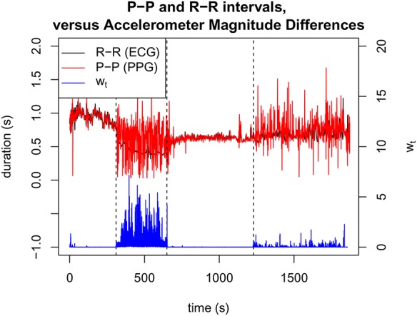
Time series of P–P and R–R intervals acquired from PPG and ECG (upper plot), and corresponding accelerometry time series $w_t$ (lower plot) for an exemplar patient, where divisions between the four sections of the experimental protocol are shown as vertical dashed lines

The figure also shows that there exist the expected differences between P–P and R–R intervals estimated from the PPG and ECG sensors. During the first and third sections, the time series of P–P and R–R intervals are similar. As motion increases, it may be seen that the fourth section corresponds to frequent substantive differences between P–P and R–R intervals, and that these differences become larger during the increased activity of the second section.

3.2. Outlier removal

Before subsequent processing we performed outlier removal to discard P–P intervals with physiologically implausible values, e.g. increased P–P intervals (and therefore HR) that occur faster than could be feasibly produced by physiology. This was straightforwardly performed by computing a 10 s moving average ${\mu }_{10}$, and then discarding P–P intervals $P{P}_t$ for which $|P{P}_t-{\mu }_{10}|\ge 0.5{\mu }_{10}$. Fig. 2 shows this pre-processing step applied to the R–R intervals obtained from the PPG, where it may be seen that the largest transients are removed.

Fig. 2.

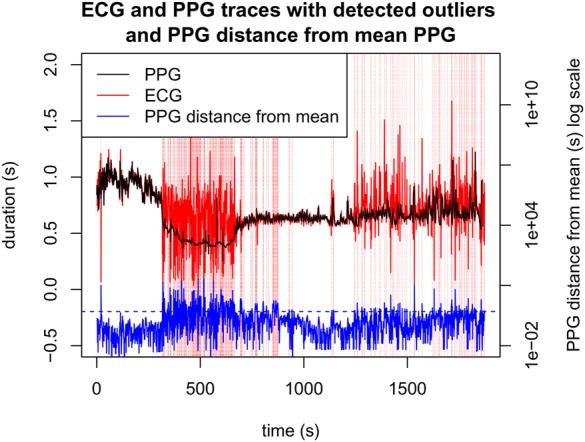
P–P intervals selected for removal (vertical red lines), and corresponding distance of instantaneous P–P interval from the 10 s moving average, as a percentage. The blue horizontal dotted line indicates the threshold for the distance to trigger an outlier detection

3.3. HRV analysis

We estimate the various HRV features defined earlier in Section 1.1, which are AverageNN, SDNN, RMSSD, pNN50, and SVI. These are estimated, together with $W_t$, over a short-time window of duration $\tau =40\mathrm{s}$, with subsequent windows overlapped by 20 s.

Fig. 3 shows HRV features estimated for an exemplar subject. During the second section of the experiment, it may be seen that the increased movement of the subject results in substantial errors in the PPG signal that propagate to the HRV features.

Fig. 3.

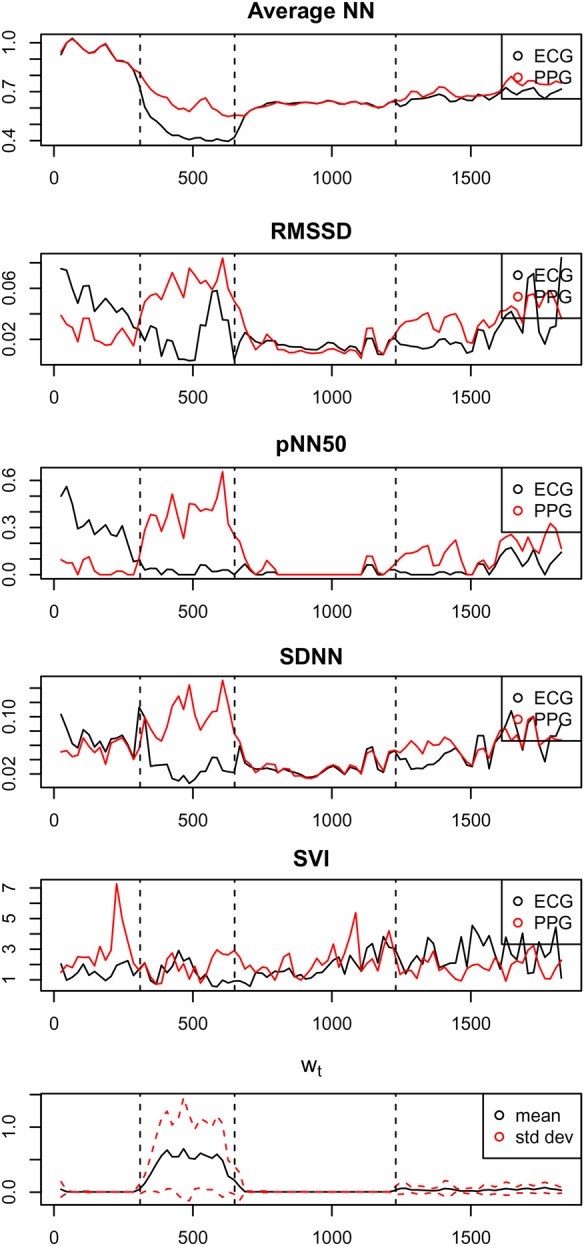
HRV features estimated from P–P intervals acquired from PPG (red) and from R–R intervals acquired from ECG (black), in reading order. The lower plot shows the time series of accelerometry $W_t$, with mean and one SD values within a window of $\tau =40\mathrm{s}$ shown in black and red, respectively

For this exemplar patient, we can see that the standard deviation of the accelerometry time series $W_t$ is correlated to the magnitude of the errors in the time-domain HRV features, with correlation coefficients: $\rho =0.91$, 0.84, 0.67, and 0.64 for AverageNN, SDNN, pNN50, and RMSSD, respectively. However, this correlation does not exist for the frequency-domain HRV feature, SVI, for which the corresponding correlation coefficient is $\rho =-0.03$. We will investigate this latter phenomenon in a subsequent section of this Letter.

3.4. Discarding data with low signal quality

Having confirmed above the intuition that error in HRV feature estimation is correlated with movement, we subsequently choose to estimate signal quality via the accelerometry time series $W_t$, such that HRV estimates may be discarded if $W_t$ exceeds some threshold $\kappa$.

We therefore calculated the distribution of error for each HRV feature, as a function of the value of $W_t$ (the average of $w_t$ over the window of duration $\tau$), and noticed that error for most of the HRV features (AverageNN, SDNN, RMSSD, and pNN50) quickly increases for $W_t>0.02$: the error for AverageNN goes from 0.0013 ($W_t<0.02$) to 0.0142 ($W_t>0.02$); the error for SDNN goes from 0.0061 ($W_t<0.02$) to 0.0139 ($W_t>0.02$); the error for RMSSD goes from 0.0079 ($W_t<0.02$) to 0.0153 ($W_t>0.02$); the error for RMSSD goes from 0.057 ($W_t<0.02$) to 0.125 ($W_t>0.02$). SVI is the only HRV feature whose error does not change with $W_t>0.02$. Following the observation that, for most of the HRV features, the error is an order of magnitude lower than the value of the corresponding HRV feature for $W_t<0.02$, and that the error becomes of the same order of magnitude as the value of the HRV feature for $W_t>0.02$, we choose a threshold of $\kappa =0.02$ for the remainder of this work. We emphasise that this is a candidate $\kappa$, given the prototype nature of the study, conducted on a small patient group, and which would naturally be more principled in formulation for a subsequent larger study.

3.5. Signal realignment

The final step in our pre-processing is to find (and correct for) any time offset that might be between the PPG and ECG. This is straightforwardly performed by comparing the pre-processed time series of P–P intervals and R–R intervals, and calculating the squared distance d between the two for a varying time offset $\alpha$. We note that the P–P and R–R intervals are not sampled at corresponding times, and therefore both waveforms were resampled at 10 Hz.

Fig. 4 shows this relationship for an exemplar patient, which is reproduced across other subjects (not shown here for brevity). We choose a value of $\alpha =2.2\mathrm{s}$, which corresponds to the value that minimises d.

Fig. 4.

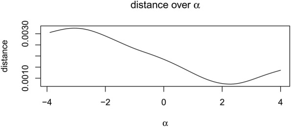
Squared distance d between pre-processed P–P and R–R intervals, as a function of time offset $\alpha$ between them (seconds)

4. Results

This section presents results of (i) investigating the effect of changing window size $\tau$ when calculating HRV features; (ii) investigating the signal-to-noise ratio (SNR) for the time series of P–P interval estimated from the PPG, with respect to the reference R–R intervals derived from the ECG; and (iii) the distribution of errors for HRV features throughout the four stages of the experimental protocol.

4.1. Effect of window size

Table 1 shows the root mean-square error (RMSE) of each HRV feature for various window sizes $\tau$. It may be seen that the RMSE does not change substantially with varying $\mathrm{tau}$; errors increase with window size for AverageNN ($\simeq 10\text{\%}$), RMSSD ($\simeq 10\text{\%}$), and pNN50 ($\simeq 2\text{\%}$), while the RMSE decreases for SDNN ($\simeq 25\text{\%}$) and SVI ($\simeq 30\text{\%}$). However, it may be seen from the table that the decrease of SVI is not proportional to changes in $\tau$.

Table 1.

RMSE of HRV features, for window size $\tau$

$\tau ,\mathrm{s}$	AverageNN	SDNN	RMSSD	pNN50	SVI
40	0.0480	0.0334	0.0564	0.2285	0.6471
60	0.0489	0.0316	0.0566	0.2294	0.5683
80	0.0499	0.0294	0.0575	0.2279	0.6080
100	0.0504	0.0287	0.0583	0.2330	0.5982
120	0.0506	0.0280	0.0575	0.2259	0.6613

It is common practice to require long-duration windows of data to estimate HRV features reliably. Our experiment shows that short-duration windows of data still allow to perform accurate estimation of time-domain HRV features.

4.2. Signal-to-noise ratio

Noting that the ECG-derived time series of R–R intervals RR is used as the reference, we can define the time series of residuals $r_t=RR-PP$, where the time series of re-aligned P–P intervals from the PPG is PP.

Fig. 5 shows the spectra of RR compared with the residual time series $r_t$ when calculated with and without pre-processing of the time series of P–P intervals derived from the PPG.

Fig. 5.

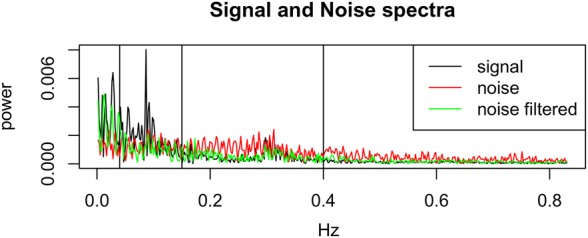
Spectra for the signal RR versus residuals $r_t$ where the latter have been calculated from the original (‘noise’) and pre-processed (‘noise filtered’) signals PP, shown in red and green, respectively. The vertical lines show the frequency bands used in HRV analysis: LF between 0.04 and 0.15 Hz, and HF between 0.15 and 0.4 Hz

Additionally, we can plot the SNR between RR (the ‘signal’) and $r_t=RR-PP$ (the ‘noise’) for the cases with and without pre-processing of PP, as shown in Fig. 6.

Fig. 6.

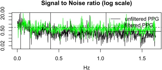
SNR between RR (signal) and residuals $r_t$ (noise), with and without pre-processing of PP shown in green and black, respectively. A horizontal line shows SNR = 1.0

Figs. 5 and 6 show that the power in the signal exceeds that of the noise for the ultra-low frequency band (i.e. those frequencies below LF). This is an expected result, because power in this band corresponds to slowly changing physiological phenomena that modulate the time series of P–P and R–R intervals (corresponding to the HR) – this corresponds to diurnal changes in blood pressure, temperature regulation, and other effects.

Both the LF and HF bands have a very low SNR. The LF band frequently exceeds SNR = 1.0 for the case in which the P–P intervals from the PPG have been pre-processed. HF band has a SNR close to, or below, SNR = 1.0, which corresponds to the fact that the noise is at least as powerful as the signal in this band. We note also that the absolute power in the HF band is low with respect to the lower-frequency bands (as shown in Fig. 5). This latter effect may explain why SVI is as unreliable as has been observed by our results: noting that SVI is the ratio between LF and HF, with HF in the denominator, it is therefore sensitive to HF noise. We may observe that the pre-processed (‘filtered’) PPG has a higher SNR than the unprocessed (‘unfiltered’) PPG in the HF band. We conclude that SVI is not a reliable HRV feature and should be used with caution, ensuring our pre-processing steps are performed.

Fig. 7 shows the distribution of SNRs for HF and LF bands across all subjects, where we emphasise that these distributions are normalised histograms. The figure shows that HF values frequently fall below the value of SNR = 1 (i.e. that part of the distribution shown in black that lies to the left of the vertical dashed line). This indicates that HF values are not reliable for the majority of patients. LF values appear to be more reliable than HF, since a larger proportion of the distribution shown in red falls above SNR = 1.

Fig. 7.

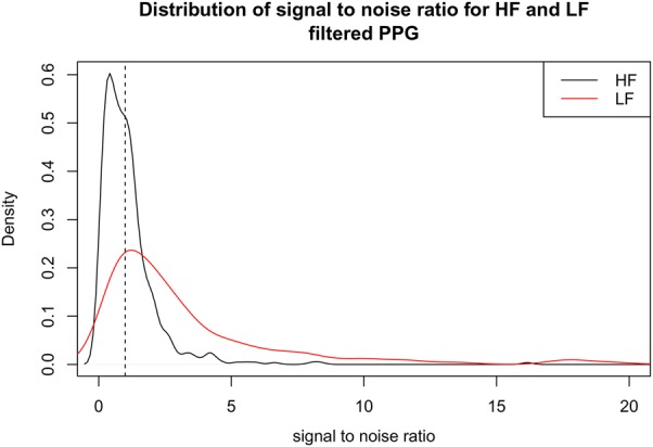
Distribution of SNR in HF and LF bands for all subjects. SNR = 1.0 is shown with the vertical dashed line; values to the left of this line correspond to a proportion of subjects’ data that falls below SNR = 1.0

4.3. Distributions of HRV errors for all subjects

In the previous sections, we applied the accelerometer-based noise filtering and subsequent HRV analysis to the data collected from a single user. In this section, we replicate the same procedure to the data collected from all users. For every HRV feature we aggregate the results and we calculate the mean, the standard deviation, the 25th, 50th, and 75th percentiles. We present those results as statistical descriptors of the expected error propagation from PPG to HRV features.

Table 2 shows the distribution of accelerometry $W_t$ over all subjects in the four stages of the experimental protocol (rest, stress, recovery, and free). As expected, the rest and recovery stages have similar accelerometry, with more than 75% of the $W_t$ values below our threshold $\kappa$ value of $W_t=0.02$). During the free stage, values of $W_t$ fall below 0.02 than 50% of the time. During the stress stage, $W_t$ consistently exceeds the threshold $\kappa$.

Table 2.

Distribution of accelerometry $W_t$, showing the mean and standard deviation (SD) across all subjects, and the quantiles on the distribution of $W_t$ at 0.1, 0.25, 0.75, and 0.9

	Mean	SD	0.25	0.5	0.75	0.9
rest	0.016	0.032	0.002	0.002	0.010	0.072
stress	0.406	0.202	0.212	0.471	0.577	0.600
recovery	0.012	0.035	0.002	0.003	0.007	0.011
free	0.052	0.032	0.027	0.057	0.075	0.089

Tables 3–6 show the distribution of errors in the time-domain HRV features, for each phase. Reflecting the distribution of the accelerometry $W_t$, the rest and recovery stages have low error most of the time (75%), the free stage has low error between 25 and 50% of the time, and the stress stage is consistently associated with large error in HRV features.

Table 4.

Distribution of SDNN error, showing the mean and SD across all subjects, and the quantiles on the distribution of SDNN error at 0.1, 0.25, 0.75, and 0.9

	Mean	SD	0.25	0.5	0.75	0.9
rest	0.012	0.011	0.004	0.009	0.016	0.022
stress	0.132	0.036	0.111	0.133	0.166	0.179
recovery	0.006	0.014	0.001	0.003	0.006	0.015
free	0.030	0.022	0.009	0.028	0.049	0.061

Table 5.

Distribution of RMSSD error, showing the mean and SD across all subjects, and the quantiles on the distribution of RMSSD error at 0.1, 0.25, 0.75, and 0.9

	Mean	SD	0.25	0.5	0.75	0.9
rest	0.025	0.014	0.016	0.024	0.031	0.038
stress	0.078	0.022	0.064	0.079	0.089	0.107
recovery	0.008	0.011	0.003	0.004	0.008	0.019
free	0.033	0.020	0.017	0.034	0.049	0.056

Table 3.

Distribution of AverageNN error, showing the mean and SD across all subjects, and the quantiles on the distribution of AverageNN error at 0.1, 0.25, 0.75, and 0.9

	Mean	SD	0.25	0.5	0.75	0.9
rest	0.004	0.010	0.001	0.001	0.002	0.008
stress	0.127	0.052	0.088	0.124	0.155	0.194
recovery	0.007	0.020	0.001	0.001	0.003	0.011
free	0.043	0.032	0.009	0.042	0.072	0.082

Table 6.

Distribution of pNN50 error, showing the mean and SD across all subjects, and the quantiles on the distribution of pNN50 error at 0.1, 0.25, 0.75, and 0.9

	Mean	SD	0.25	0.5	0.75	0.9
rest	0.238	0.107	0.167	0.235	0.293	0.377
stress	0.511	0.086	0.438	0.525	0.565	0.634
recovery	0.021	0.049	0.000	0.000	0.030	0.060
free	0.174	0.116	0.076	0.165	0.260	0.332

Table 7 shows the error associated with the frequency-domain HRV feature, SVI. As concluded previously, this feature appears to be generally less reliable than the time-domain HRV features, across all subjects. The large errors present in the estimation of SVI, reported in Table 7, are due to the low SNR of the HF band.

Table 7.

Distribution of SVI error, showing the mean and SD across all subjects, and the quantiles on the distribution of SVI error at 0.1, 0.25, 0.75, and 0.9

	Mean	SD	0.25	0.5	0.75	0.9
rest	1.536	1.298	0.745	1.022	2.099	2.377
stress	0.611	0.535	0.147	0.451	0.772	1.515
recovery	0.659	0.452	0.332	0.537	0.932	1.390
free	1.308	0.994	0.512	1.112	2.057	2.948

5. Conclusions

We have shown that PPG data acquired from a consumer-grade wrist-worn wearable device are highly susceptible to motion artefacts. We have analysed the noise profile, and shown that the frequency-domain HRV feature SVI is not reliable, because the SNR in the HF band (which is in the denominator of the quotient that defines SVI) often falls below a value of SNR = 1.0.

Our results demonstrate that HRV features extracted when the user is still reliable, even if the user is not in a cardiovascular stationary state (such as in the third stage of our experimental protocol, ‘recovery’), which therefore does not agree with the findings described in the literature [20].

We have shown that it is possible to use the accelerometry $W_t$ derived from the wearable device to estimate the quality of the corresponding PPG signal. Therefore, unreliable data can automatically be discarded according to a threshold $\kappa$ on $W_t$. Such an operation could be used to selectively turn off the PPG sensor, thereby saving battery life on the wearable device, and also avoiding HRV analysis using unreliable data. We derive a value of $\kappa$ that retain data with error an order of magnitude lower than the signal for most HRV features, discarding data with higher error. The value of $\kappa$ should be refined with a larger dataset.

We have shown that the conventional use of long-duration windows of data is not needed to perform accurate estimation of time-domain HRV features.

We emphasise that the results described in this report represent a preliminary study, and planned future work includes validation of these results with more subjects to verify our findings.

6. Funding and declaration of interests

Dr Clifton reports personal fees from BioBeats Ltd. during the conduct of the study.

Supplementary Material

Sup 1

Supplementary Data