Abstract
Positron Emission Tomography (PET) is a functional imaging modality widely used in oncology, cardiology, and neuroscience. It is highly sensitive, but suffers from relatively poor spatial resolution, as compared with anatomical imaging modalities, such as magnetic resonance imaging (MRI). With the recent development of combined PET/MR systems, we can improve the PET image quality by incorporating MR information into image reconstruction. Previously kernel learning has been successfully embedded into static and dynamic PET image reconstruction using either PET temporal or MRI information. Here we combine both PET temporal and MRI information adaptively to improve the quality of direct Patlak reconstruction. We examined different approaches to combine the PET and MRI information in kernel learning to address the issue of potential mismatches between MRI and PET signals. Computer simulations and hybrid real patient data acquired on a simultaneous PET/MR scanner were used to evaluate the proposed methods. Results show that the method that combines PET temporal information and MRI spatial information adaptively based on the structure similarity index (SSIM) has the best performance in terms of noise reduction and resolution improvement.
Index Terms: Positron emission tomography, Patlak direct reconstruction, Kernel method, MRI, structure similarity
I. Introduction
Positron Emission Tomography (PET) can produce three dimensional functional images of a living subject through the injection of a radioactive tracer. It has wide applications in oncology [1], cardiology [2] and neurology [3]. Though PET is highly sensitive, in the picomolar range, the image quality is still limited by various resolution degradation factors [4]. Compared with PET, x-ray Computed Tomography (CT) and Magnetic Resonance Imaging (MRI) have better anatomical image resolution. With the wide availability of PET/CT and the new arrival of PET/MR systems, anatomical information from CT or MRI are readily available for use in the PET reconstruction. Research in this area has been going on for decades and different methods have been developed based on approaches such as mutual information or joint entropy [5]–[7], segmentation or boundary extraction [8]–[12], gradient information from a prior image [13], [14], intensity similarity in a prior image [15]–[19], wavelet [20], dictionary learning [21], [22], image sparse representation [23], convolutional neural network [24] and the kernel method [25]–[28]. The kernel method is a well-studied framework in machine learning that implicitly transfers the raw data points to a higher dimensional feature space using a kernel function. It has recently been applied to dynamic image reconstruction [25] and successfully extended to MRI aided PET reconstruction [26]–[28].
Here we combine the above two approaches to further improve the quality of dynamic PET reconstruction. Compared with static PET, dynamic PET provides additional temporal information of the tracer kinetics, which can be useful for tumor detection and treatment monitoring [29]–[31]. Conventionally dynamic PET images are reconstructed frame by frame, and time activity curves (TAC) from regions of interest (ROI) or individual pixels are fitted to a linear or nonlinear kinetic model. Direct reconstruction methods have been developed recently to estimate parametric images directly from the measured sinogram by combining the PET imaging model and tracer kinetics in an integrated framework [32]–[36]. It has been shown that direct reconstruction methods can reduce noise amplification compared with traditional indirect methods [37]. Anatomical information can be used to regularize the parametric images in direct reconstruction [28], [38], [39]. In this work, we focus on the Patlak model [40]–[44], which is a widely used graphical model. The slope of Patlak plot is a useful quantitative metric when the tracer uptake is irreversible. One challenge in using anatomical information in PET reconstruction is that there are often mismatches between MRI and PET signals in real data. For example, tumor regions showing up in a PET image may not appear in a co-registered MRI image [45]. It is thus crucial to account for this mismatch by exploiting both anatomical and PET information to construct the kernel matrix. In a previous work [27], spectral models were employed to model the PET temporal information and the kernel matrix were constructed using MRI information. The work here aims at combining the MRI based kernel matrix and dynamic PET based kernel matrix adaptively using a local similarity measure.
The main contributions of this paper include (1) combining the PET information and the MRI information adaptively based on local similarity and (2) applying this hybrid kernel to the direct Patlak reconstruction. This paper is organized as follows. Section 2 introduces the Patlak model and the kernel method. Section 3 describes the computer simulations and hybrid real data used in the evaluation. Experimental results are shown in section 4, followed by discussions in section 5. Finally conclusions are drawn in Section 6.
II. Method
A. Dynamic PET model
Dynamic PET data in the kth time frame, yk ∈ ℝM × 1, can be modeled as a collection of independent Poisson random variables with the mean ȳk ∈ ℝM × 1 related to the unknown tracer distribution in the kth time frame, xk ∈ ℝN × 1, through an affine transform
| (1) |
where Nk ∈ ℝM × M is the time dependent normalization matrix. P ∈ ℝM × N is the detection probability matrix with the (i, j)th element pij being the probability of detecting a photon pair produced in voxel j by detector pair i. sk ∈ ℝM × 1 and rk ∈ ℝM × 1 denote the expectation of scattered and random coincidences, respectively, in the kth time frame. M is the number of lines of response (LOR) and N is the number of image voxels. When concatenating T time frames together, we can get
| (2) |
where N = diag[N1, N2, …NT], ⊗ denotes the Kronecker product, IT is a T × T identity matrix, , , , , and “′” denotes matrix or vector transpose. Let denote the measured dynamic data. The log-likelihood function of y can be written as
| (3) |
The maximum likelihood estimate of the unknown image x can be found by
| (4) |
B. Patlak model
The Patlak graphical method [40] has been widely used for compartment models that contain at least one irreversible compartment. Under this model, the tracer concentration at time t, c(t) ∈ ℝN × 1, can be represented by a weighted sum of the blood input function Cp(t) and its integral after a sufficient length of time t⋆ as
| (5) |
where κ ∈ ℝN × 1 is the Patlak slope image and b ∈ ℝN × 1 is the Patlak intercept image. The Patlak slope image κ can reflect the influx rate of the PET tracer and is a very important quantitative metric in practice. Considering the radioactive decay, the image intensity at the kth frame, xk, can be expressed as
| (6) |
where ts,k and te,k are the start time and end time of frame k, λ is the decay constant of the PET tracer, and
| (7) |
| (8) |
Putting all time frames together, we can have
| (9) |
where θ = [κ′, b′]′, IN is an N × N identity matrix, and
| (10) |
Conventionally, images are reconstructed frame-by-frame according to (4) and then the Patlak parameters are estimated by fitting the time activity curves to the Patlak model (9). The least squares solution of the fitting is
| (11) |
C. Direct reconstruction using the kernel method
Here we choose the direct reconstruction approach by substituting the Patlak graphical model (9) into (2) to get:
| (12) |
Previously efforts have been made to add regularization in the parametric space by using a penalty function, which aims to enforce smoothness inside the region and allow sharp transition near the edges [38], [39]. Here we choose to regularize the direct reconstruction through the use of a kernel matrix [25]. The main idea is to represent the unknown parametric images by a linear combination of transformed features calculated from prior information. Using the kernel trick, we can express the Patlak slope and intercept images as
| (13) |
| (14) |
where K ∈ ℝN × N is the kernel matrix, ακ ∈ ℝN × 1 and αb ∈ ℝN × 1 denote the kernel coefficient vectors of κ and b, respectively. Construction of the kernel matrix K is described in Section II.D. Here the same kernel matrix is used for the Patlak slope and intercept because we expect that they share the same regional boundaries, although they may have different intensities and contrasts. However, the proposed algorithm is amendable to use different kernel matrices for the Patlak slope and intercept, if necessary. In the implementation, we require the kernel coefficients to be non-negative, which guarantees non-negative Patlak slope and intercept. Defining , θ can be expressed as
| (15) |
Substituting (15) into (12), we get
| (16) |
| Algorithm 1 Algorithm for direct Patlak reconstruction using the kernel method | |
| Input: Maximum iteration number MaxIt, sub-iteration number SubIt, starting time frame FraSta and ending time frame FraEnd | |
| 1: | Initialize α0, SllbIt = 1N |
| 2: | for n = 1 to MaxIt do |
| 3: | xn (A ⊗ K)αn–I, SubIt |
| 4: | αn,0 = αn–I, SubIt |
| 5: | for k = FraSta to FraEnd do |
| 6: | |
| 7: | end for |
| 8: | for q = 1 to SubIt do |
| 9: | , where 1MT is a MT × 1 all-one vector. |
| 10: | end for |
| 11: | end for |
| 12: | return θ̂ = (I2 ⊗ K)α̂MaxIt,SubIt |
where we use the following property of Kronecker product
| (17) |
To estimate α, we use the nested EM algorithm [46] for faster convergence. The resulting algorithm flowchart is shown in Algorithm 1.
D. Kernel construction
Following the original paper [25], we use a radial Gaussian kernel. The (i, j)th element of the kernel matrix K is
| (18) |
where fi ∈ ℝNf × 1 and fj ∈ ℝNf × 1 represent the feature vectors of voxel i and voxel j, respectively, σ2 is the variance of the image and Nf is the number of voxels in a feature vector. Two types of feature vectors have been proposed before. In [25], one-hour long dynamic PET data were re-binned into three twenty-minutes frames and the reconstructed images , m = 1, 2, 3, were used to form the feature vectors ,
| (19) |
Hereinafter, this method is referred to as KPET. The second method extracts the feature vectors from a co-registered MR image [26], [27],
| (20) |
where (xM)i is a local patch centered at voxel i from the MR image. This method is referred to as KMRI. In this paper, a 3×3×3 local patch was extracted for each voxel to form the feature vectors. Before the feature extraction, the re-binned PET images and MR image were normalized so that the image standard variation inside the brain region is 1 and we set σ = 1 in (18).
As shown in previous publications [26], [27], KMRI can preserve sharp boundaries in PET images. However, it can also introduce bias when PET tracer uptake does not share the same boundary with the MRI image. A better approach is to combine the two types of kernels so that we can minimize the risk of smoothing out PET signals while exploiting anatomical information from KMRI. An intuitive choice is to weight MRI and PET features equally, which we refer to as K-PET-MRI-0.5. This method would unfortunately reduce the image quality in the regions where PET image and MRI image share same boundaries compared with that using the KMRI alone, because PET features are often noisier than MRI features. A better approach is to assign a spatially variant weight to PET and MRI features based on a similarity measure ρ. Ideally the similarity measure ρ should be high (close to 1) in regions where PET and MRI images share the same boundary and be low (close to 0) in regions where their boundaries do not match.
Given a good similarity measure, we can weight PET and MRI features based on the similarity. The hybrid kernel matrix is then formed as
| (21) |
where
| (22) |
The factor 3 is included because there are three PET images in (19) and only one MRI image in (20). When multiple MRI images are available (e.g., [47]), the factor should be adjusted accordingly. Equation (22) is constructed so that Dij is symmetric.
A crucial task is to find an appropriate similarity measure ρ. We studied two approaches to calculating ρ. The first one was based on the correlation between the PET kernel and MRI kernel vectors [48] and the second method was based on the structural similarity [49] between the reconstructed images of the last frame data using KPET and KMRI. We found that the kernel-correlation based result is not always satisfactory as the correlation between matched flat regions is dominated by image noise. Therefore, we focus on the structural similarity based method in this paper. This method is referred to as K-PET-MRI-S.
The structural similarity (SSIM) index [49] is a widely used image quality index for comparing images. Before calculating the SSIM index map, the input images are scaled to have a mean value of one inside the brain regions. Given two local patches extracted from the input images, x and y, the general definition of SSIM is
| (23) |
where , and are the luminance, contrast and similarity measures. Here μx, μy, , are the means and variances of x and y, and σxy is the covariance between x and y. To avoid block artifacts, neighboring voxels are weighted by an isotropic Gaussian function. The standard deviation of the Gaussian function was set to 1 pixel in our experiment, because we found that the default value (1.5 pixels) suggested by [49] resulted in a blurry SSIM map for our application. C1, C2 and C3 are small constants used to stabilize the results. We used the MATLAB implementation [49] with C1 = (0.01L)2, C2 = (0.03L)2 and C3 = C2/2, where L is a constant value. Based on our observations, the most influencing component of SSIM(x, y) for distinguishing an unmatched region from matched regions is the similarity measure s(x, y). Hence we fixed α and β to 1 and adjusted γ and L. We evaluated the mean SSIM values for a simulated unmatched tumor region and matched normal region for a wide range of γ and L values. We found that setting γ = 12 and L = 50 is a reasonable choice, which resulted in a low SSIM value for the unmatched regions while keeping the SSIM value for the matched regions to be greater than 0.95. More details of the calculation are given in the supplemental materials.
After obtaining SSIM index, we calculate ρ by scaling the SSIM index
| (24) |
where C was set to 0.2. The reason for scaling is that the minimum value of the SSIM value is around 0.2 while the range of ρi should be between 0 and 1.
For efficient computation, all kernel matrices were constructed using a K-Nearest-Neighbor (KNN) search in a 7×7×7 search window with K = 50, i.e.,
| (25) |
Following [25], all kernel matrices were normalized by
| (26) |
and K̄ was then used in the image reconstruction.
III. Experiment evaluations
A. Computer simulation study
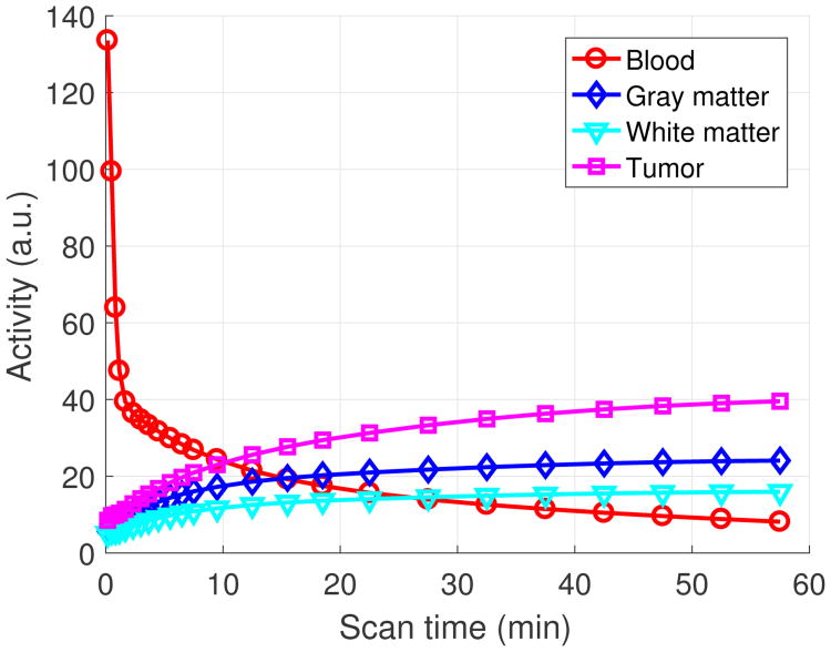
A 3D brain phantom from the Brainweb [50] was used in the simulation study. The scanner geometry models a Siemens mCT scanner [51]. The system matrix P was computed by using the multi-ray tracing method [52]. The image matrix size is 125 × 125 × 105 and the voxel size is 2 × 2 × 2 mm3. The time activity curves of the gray matter and white matter were generated mimicking an FDG scan using a two-tissue-compartment model with the kinetic parameters shown in Table I and an analytic blood input function [53] in Fig. 1. To simulate mismatches between the MR and PET images, twelve hot spheres of diameter 16 mm were inserted into the PET image as tumor regions, which are not visible in the MR image. The dynamic PET scan was divided into 24 time frames: 4×20 s, 4×40s, 4×60 s, 4×180 s, and 8×300 s. For the direct Patlak reconstruction, only the last 5 frames for a total duration of 25 minutes were used. Three orthogonal slices of the MRI prior image, PET attenuation map and PET activity image at the 24th frame are shown in Fig. 2. Noise-free sinogram data were generated by forward-projecting the ground-truth images using the system matrix and the attenuation map. Poisson noise was then introduced to the noise-free data by setting the total count level to be equivalent to an 1-hour FDG scan with 5 mCi injection. Uniform random events were simulated and accounted for 30 percent of the noise free data in all time frames. Scatters were not simulated in this study. During image reconstruction, the blood input function and all the correction factors were assumed to be known exactly. Apart from the tumor study, we also performed an neural activation simulation study by simulating the activation regions according to [17]. Results are shown in the supplemental materials.
Table I. The simulated kinetic parameters of FDG.
| Tissue | fυ | K1 | k2 | k3 | k4 |
|---|---|---|---|---|---|
| Gray matter | 0.03 | 0.071 | 0.086 | 0.055 | 0.001 |
| White matter | 0.03 | 0.046 | 0.080 | 0.052 | 0.001 |
| Tumor | 0.05 | 0.082 | 0.055 | 0.085 | 0.002 |
Fig. 1.
The simulated time activity curves.
Fig. 2.
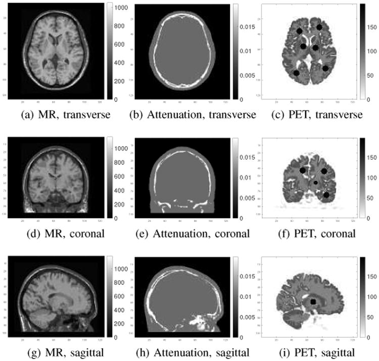
Three orthogonal slices of the MR prior image (first column), attenuation map (second column) and the 24th frame of the PET ground truth image (third column).
To quantify the noise properties across different realizations, multiple independent and identically distributed (i.i.d.) dynamic data sets were generated. The KPET kernel matrix and the hybrid kernels were calculated for each realization. The KMRI kernel matrix was kept the same in all realizations. When constructing the PET features for each realization, the first, second and last twenty-minutes frames were reconstructed using the ordered-subsets EM (OSEM) algorithm (10 iterations and 6 subsets), and smoothed by a Gaussian filter with a FWHM of 3 mm. We then used the kernels to reconstruct the last static frame as well as to perform the direct Patlak reconstruction using the last 5 frames. For the static reconstruction, 20 iterations with 6 subsets were run, while for the direct Patlak reconstruction, 100 iterations of the nested EM algorithm with Ns = 3 sub-iterations were run.
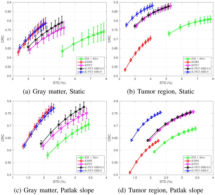
For quantitative comparison, contrast recovery coefficient (CRC) vs. the standard deviation (STD) curves were plotted. The CRC was computed between selected gray matter regions and white matter regions as
| (27) |
Here R is the number of realizations, which is equal to 50 in both the static reconstruction and the direct Patlak reconstruction. is the average uptake of the gray matter over Ka ROIs in realization r. The ROIs were drawn in both matched gray matter regions and the unmatched tumor regions. The reason to quantify both the gray matter and tumor regions is to compare the performance of different methods under the situations with either matched or unmatched MR information. For the case of matched gray matter, we had Ka = 10, and for the unmatched tumor regions, we had Ka = 12. When choosing the matched gray matter regions, only those pixels inside the predefined 20-mm-diameter spheres and containing 80% of gray matter were included. is the average value of the background ROIs in realization r, and Kb = 37 is the total number of background ROIs. The background ROIs were 12-mm spheres drawn in the white matter. The background STD was computed as
| (28) |
where is the average of the kth background ROI over realizations, and Kb = 37 is the total number of background ROIs.
B. Hybrid real data
A 70-minutes dynamic FDG PET scan of a human subject was acquired on a Siemens Brain MR-PET scanner after a 5-mCi injection. The dynamic PET data were divided into 25 frames: 4×20 s, 4×40 s, 4×60 s, 4×180 s, 8×300 s and 1×600 s. The data were reconstructed into an image array of 256×256×153 voxels with a voxel size of 1.25 × 1.25 × 1.25 mm3 using different kernel matrices as those used in the simulation study. Correction factors for randoms, scatters were estimated using the standard software provided by the manufacturer and included in the forward model during reconstruction [54], [55]. The motion correction was performed in the LOR space based on the simultaneously acquired MR navigator signal [56]. Attenuation was derived from a T1-weighted MR image using the SPM based atlas method [57]. The first 20-minutes, middle 20-minutes and last 30-minutes PET data were reconstructed separately to form the PET features. The MR features were extracted from the T1-weighted MR image, which has the same voxel size as the PET images. To obtain the blood input function, blood regions were segmented from the MR image by thresholding inside a predefined mask as the blood vessel is bright in the T1-weighted MR image. The blood input function was then computed from the frame-by-frame OSEM reconstruction. A maximum intensity projection of the segmented blood region overlaid with the MRI image is shown in Fig. 3(a) and the extracted blood input function without decay correction is shown in Fig. 3(b). As the ground truth of the regional uptake is unknown, a hot sphere of diameter 12.5 mm, mimicking a tumor, was added to the PET data (invisible in the MRI image). It simulates the case where MRI and PET information does not match. The location of the tumor is shown in Fig. 7. The TAC of the hot sphere was set to the TAC of the gray matter, so the final TAC of the simulated tumor region is higher than that of the gray matter because of the superposition. The simulated dynamic tumor images were forward-projected to generate a set of noise-free sinograms, taking into account of detector normalization and patient attenuation. Randoms and scatters from the inserted tumor were not simulated because they would be negligible compared with the scattered and random events from the patient background. Poisson noise was then introduced and finally the tumor sinograms were added to the original patient sinograms to generate the hybrid real data sets. Apart from the inserted tumor, the left putamen region was also used in the quantification, considering only its absolute uptake as the ground truth is unknown. The Patlak plots of the left putamen and the inserted tumor along with the fitted lines are shown in Fig. 3(c,d), respectively, which indicate that the Patlak model is reasonable.
Fig. 3.
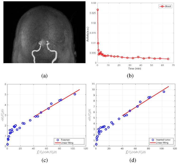
(a) The segmented MRI blood vessels; (b) The extracted blood input curves based on the MRI segmented vessels; (c) The Patlak plot for the left putamen TAC; and (d) the Patlak plot for the inserted tumor TAC.
Fig. 7.

The similarity maps used in K-PET-MRI-S for the hybrid real patient data. The tumor region is marked by the black circles and also indicated by the arrows.
We evaluated both the static reconstruction and direct Patlak reconstruction. To generate multiple realizations for the static reconstruction, the last 40 minutes PET data were pooled together and resampled with a 3/40 ratio to obtained 50 i.i.d. datasets that mimic 3-minutes frames. Specifically, for every list-mode event, we generated a random number uniformly distributed between 0 and 1 and the event was accepted only if the random number is less than 3/40 [58]. This process was repeated 50 times. The data were reconstructed using different methods to compare the bias versus standard deviation curves of the tumor uptake.
For the direct Patlak reconstruction, the last six dynamic frames were used. For each frame, 50 independent realizations were generated by randomly sampling the data with a 1/5 ratio. The resampled data mimic a set of dynamic data with a 1-mCi FDG injection. For tumor quantification, images with and without the inserted tumor were reconstructed and the difference was taken to obtain the tumor only image and compared with the ground truth. The tumor contrast recovery was calculated as
| (29) |
where l̄r is the mean tumor intensity inside the tumor ROI, ltrue is the ground truth of the tumor intensity, and R is the number of the realizations. For the background, 23 spherical ROIs with a diameter of 12.5 mm were drawn in the white matter and the standard deviation was calculated according to (28).
IV. Results
A. Simulation results
Fig. 4 shows the similarity map computed in K-PET-MRI-S. Most tumor regions are successfully identified by low values in the similarity map. The region in the coronal slice that shows low similarity but is outside the tumor region is caused by the blurring of a low-similarity tumor region in a neighboring coronal slice. Fig. 5 shows three orthogonal slices of the Patlak slope images reconstructed by different methods together with the ground truth images. Besides kernel based reconstructions, we also included the post-smoothed direct EM reconstruction (denoted by ‘EM+filter’). Note that the direct EM reconstruction was simply a special case of the kernel EM algorithm given in Algorithm 1 with K = I. A Gaussian filter was used to reduce the variance of the direct EM reconstruction to a comparable range to the kernel methods. By visual inspection, the Patlak slope image reconstructed using KMRI has a higher resolution than the KPET method. The fine details are also preserved by the hybrid kernels as pointed by the arrows.
Fig. 4.
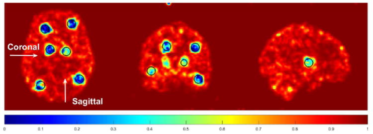
The similarity maps used in K-PET-MRI-S for the simulated data set. Circles indicate the locations of the inserted tumors.
Fig. 5.
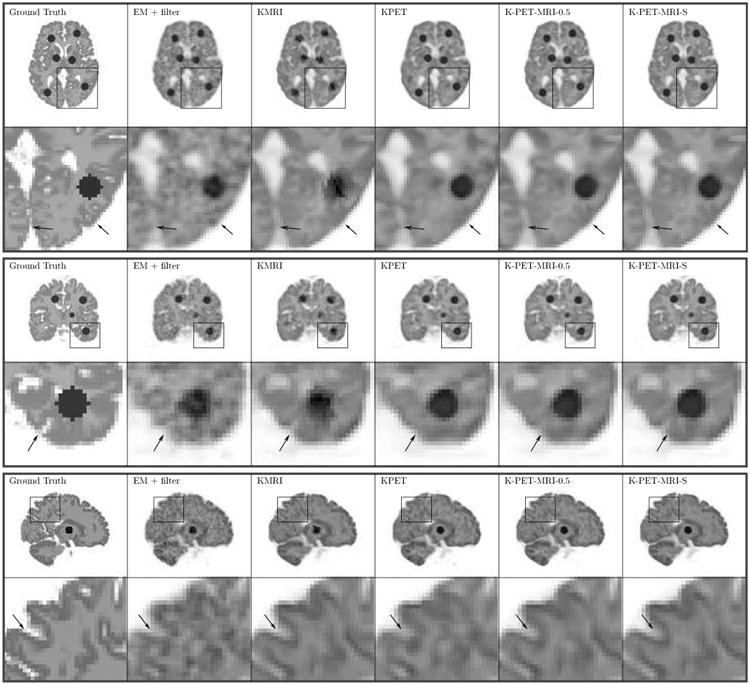
Three orthogonal slices of the reconstructed Patlak slopes using different methods for the simulation dataset.
Fig. 6 shows the CRC vs. STD curves for the matched gray-matter regions and tumor regions in the last static frame and the Patlak slope images. The error bars depict the standard deviation of the CRC values computed from 50 independent realizations (the gray-matter regions have larger error bars than the tumor regions because the tumor regions have more voxels and also higher intensity). We can see that for the matched gray-matter regions, KMRI method has the highest CRC value. The performance of K-PET-MRI-S is very close to that of KMRI. Both have much lower noise than either K-PET-MRI-0.5 and KPET, which are better than the EM + filter. For the tumor regions that are not visible in the MRI prior image, KMRI method has the lowest CRC, while KPET and K-PET-MRI-0.5 have higher CRC but also higher noise. By using the spatially adaptive weighting, K-PET-MRI-S achieves a slightly higher CRC than both KPET and KMRI while keeping the noise at the same level as that of KMRI. The noise in K-PET-MRI-0.5 method is very close to that of the KPET method because the MRI intensity in the white matter is almost uniform and does not have much influence in determining the kernel matrix when combined with PET features with equal weights. Overall, the K-PET-MRI-S method has the best performance.
Fig. 6.
CRC-STD curves at the gray matter region (left column) and the tumor region (right column) for the last frame reconstruction (top row) and the Patlak direct reconstruction (bottom row). For the static results, markers are plotted every two iterations with the lowest point corresponding to the 6th iteration. For the Patlak results, markers are plotted every ten iterations with the lowest point corresponding to the 30th iteration.
B. Hybrid real data results
Fig. 7 shows the similarity map in K-PET-MRI-S for the hybrid real data. The artificially inserted tumor was successfully identified by low similarity values. In other regions, we can see that the similarity values are lower than those of the simulation data. This could be caused by mismatch between the real MRI and PET data. Fig. 8 shows the reconstructed Patlak slope images of the patient data by different methods. Using the KMRI method, the cortices can be seen more clearly, but the shape of the tumor is distorted as the spherical tumor does not exist in the MRI image. The KPET method can preserve the spherical shape of the tumor, but the details of the cortex are lost. By using the hybrid kernels, the shapes of both the cortexand the tumor can be recovered.
Fig. 8.
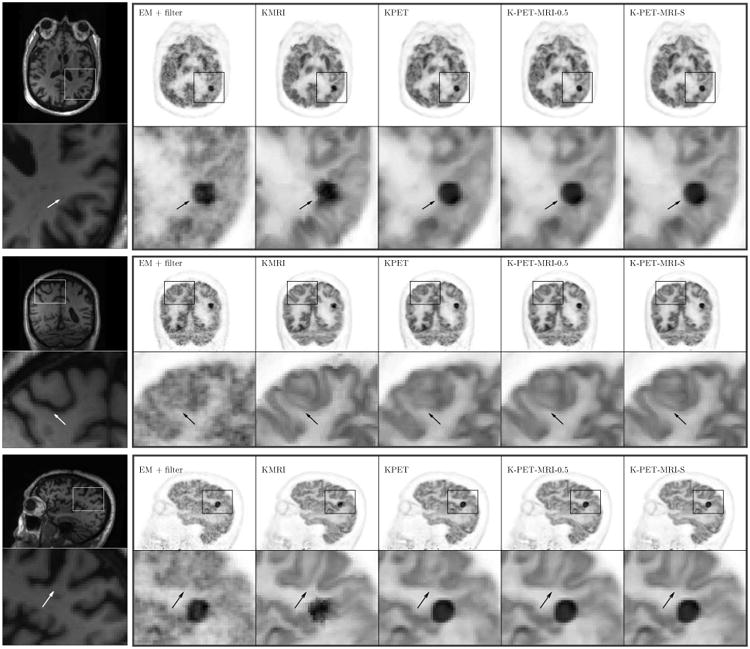
Three orthogonal slices of the reconstructed Patlak slopes for the hybrid real patient data. The first column is the MR prior image.
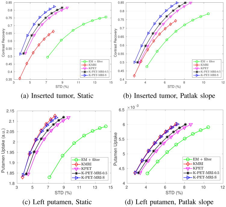
Fig. 9 shows the tumor constrast recovery vs. STD curves, as well as the left putamen absolute uptake vs. STD curves, for the last frame static reconstruction and Patlak direct reconstruction. For the tumor region, we can see that KMRI method has the lowest noise, but also the lowest uptake ratio. KPET has higher contrast, but also higher noise. The performance of K-PET-MRI-0.5 is slightly better than that of KPET, but the noise is still higher than that of KMRI. Among all the methods, K-PET-MRI-S has the best performance with the high contrast close to that of KPET and low noise close to that of KMRI.
Fig. 9.
Quantification results of the hybrid real dataset for (a,c) last frame static reconstruction (markers are plotted for every iteration with the lowest point corresponding to the third iteration) and (b,d) Patlak direct reconstruction (markers are generated for every ten iterations with the lowest point corresponding to the 30th iteration).
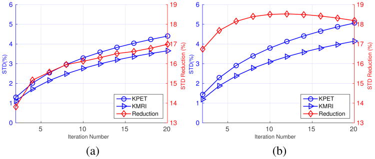
Comparing the results in Fig. 6 and Fig. 9, we can see that the noise reduction between the KMRI method and the KPET method is larger in the simulation than in the real data. We hypothesized that the reason for the difference was that the KPET kernel was recomputed for each realization in the simulation study while it was computed once using the full dynamic data in the real data experiment. This kernel variability in the simulation study introduces extra fluctuations in the reconstructed images of KPET. To test this hypothesis, we reprocessed the simulation data using the same procedure used in the real data experiment: (1) in the static reconstruction, 5 min data set were resampled from the last 40 min scan; (2) in the direct Patlak reconstruction, each of the last five frames was resampled to one-fifth of the events. The KPET kernel was computed once using the 60-minute data. Fig. 10 shows the noise comparison between KPET and KMRI methods using the resampling approach with a fixed KPET kernel. In static reconstruction, the noise reduction between KMRI and KPET is 16% (down from 25% in Fig. 6), and in the Patlak direct reconstruction, the noise reduction factor is 17% (down from 37% in Fig. 6). These values are consistent with the noise reduction factors that we saw in the real data experiment (Fig. 9).
Fig. 10.
Noise comparison between KPET and KMRI using the resampling method and a fixed KPET kernel. (a) Static image. (b) Patlak slope image. The red diamonds represent the noise reduction factor between KMRI and KPET.
V. Discussion
From the simulation data sets, we found that the noise reduction by KMRI over KPET is greater in the Patlak reconstruction than in the static reconstruction. In static reconstruction the noise reduction by KMRI over KPET is 25%, while in Patlak direct reconstruction the noise reduction by KMRI over KPET is 37%. This means including MRI information can have a greater impact on the Patlak direct reconstruction than on static reconstruction. One possible explanation for this is that in Patlak reconstruction, temporal information has been exploited through the Patlak model and the effect of temporal information derived from KPET is not as helpful as that in static reconstruction. In comparison, the noise reduction by KMRI over the direct EM reconstruction is less affected by the Patlak model than that of KPET because MRI information is separate from PET data.
In the simulation study, all reconstruction methods used the same system model that was used for the data generation, so the inconsistency in the data was solely due to Poisson noise. In the hybrid real data experiment, the reconstruction model was a ray-tracing model, since we do not know the true system model of the real scanner. Therefore, in addition to statistical noise, there also existed modeling error in the real data experiment. Despite the difference between the computer simulation and real data experiments, the proposed method worked reasonably well in both situations, demonstrating its robustness to the change of the system model used in reconstruction. While we did not use time-of-flight (TOF) information in our study, the proposed method can be directly applied to TOF reconstruction by adopting a TOF-based system model. There would be no change to the kernel matrix calculation because it is performed in the image space.
When combining MRI and PET information, assigning an equal weight to MRI and PET features (K-PET-MRI-0.5) can reduce the bias caused by missing information in the MRI prior image. However, for matched regions, K-PET-MRI-0.5 cannot fully take advantage of the MRI information. This is the reason that the K-PET-MRI-0.5 method does not improve the noise performance very much compared with the KPET method. KPET-MRI-S method uses SSIM as an index to compute the similarity between the last-frame reconstructions of KPET and KMRI methods. The SSIM method works well to identify the mismatched regions in both simulation and real data sets. As a result, K-PET-MRI-S achieved the best performance among all methods. In the real data experiment, we did observe low similarity regions outside the artificially inserted tumor. Currently, we cannot verify whether they were caused by real difference between MRI and PET information, or by the instrumentation resolution difference. More real data evaluation is needed to answer this question.
Finally, we note that for dynamic PET studies, motion correction may be necessary due to involuntary subject movements during long dynamic scans. In our study, the real PET data were corrected for motion using a simultaneously acquired MR navigator signal [56]. When we applied the kernel methods to patient data without MR-guided motion correction, we observed MR-induced artifacts in KMRI reconstructed images, possibly due to mismatches between MRI and PET data.
VI. Conclusion
We have proposed a hybrid kernel approach to direct Patlak reconstruction using both PET and MRI information. The results from simulation and real data experiments show that the proposed K-PET-MRI-S method provides a robust way to handle the potential mismatch between MRI and PET data while using matched MRI information to improve image quality. Future work will include more clinical evaluations.
Supplementary Material
Acknowledgments
This work is supported by the National Institutes of Health under grant number R01EB014894, R24MH106057 and R01EB000194. KT Chen was supported by Department of Defense (DoD) through the National Defense Science and Engineering Graduate Fellowship (NDSEG) Program.
Footnotes
Digital Object Identifier: 10.1109/TMI.2017.2776324
Contributor Information
Kuang Gong, Department of Biomedical Engineering, University of California, Davis, CA 95616 USA.
Jinxiu Cheng-Liao, Department of Biomedical Engineering, University of California, Davis, CA 95616 USA.
Guobao Wang, Department of Radiology, School of Medicine, University of California-Davis, Sacramento, CA 95817 USA.
Kevin T. Chen, Martinos Center for Biomedical Imaging, Department of Radiology, Massachusetts General Hospital and Harvard Medical School, Charlestown, MA 02129 USA
Ciprian Catana, Martinos Center for Biomedical Imaging, Department of Radiology, Massachusetts General Hospital and Harvard Medical School, Charlestown, MA 02129 USA.
Jinyi Qi, Department of Biomedical Engineering, University of California, Davis, CA 95616 USA.
References
- 1.Beyer T, Townsend DW, Brun T, Kinahan PE, et al. A combined PET/CT scanner for clinical oncology. Journal of Nuclear Medicine. 2000;41(8):1369–1379. [PubMed] [Google Scholar]
- 2.Machac J. Cardiac positron emission tomography imaging. Seminars in Nuclear Medicine. 2005;35(1):17–36. doi: 10.1053/j.semnuclmed.2004.09.002. [DOI] [PubMed] [Google Scholar]
- 3.Gong K, Majewski S, Kinahan PE, Harrison RL, et al. Designing a compact high performance brain pet scanner-simulation study. Physics in Medicine and Biology. 2016;61(10):3681. doi: 10.1088/0031-9155/61/10/3681. [DOI] [PMC free article] [PubMed] [Google Scholar]
- 4.Gong K, Zhou J, Tohme M, Judenhofer M, et al. Sinogram blurring matrix estimation from point sources measurements with rank-one approximation for fully 3d pet. IEEE Transactions on Medical Imaging. 2017 doi: 10.1109/TMI.2017.2711479. [DOI] [PMC free article] [PubMed] [Google Scholar]
- 5.Nuyts J. The use of mutual information and joint entropy for anatomical priors in emission tomography. 2007 IEEE Nuclear Science Symposium Conference Record. 2007;6:4149–4154. IEEE. [Google Scholar]
- 6.Tang J, Rahmim A. Bayesian pet image reconstruction incorporating anato-functional joint entropy. Physics in Medicine and Biology. 2009;54(23):7063. doi: 10.1088/0031-9155/54/23/002. [DOI] [PMC free article] [PubMed] [Google Scholar]
- 7.Somayajula S, Panagiotou C, Rangarajan A, Li Q, et al. PET image reconstruction using information theoretic anatomical priors. IEEE Transactions on Medical Imaging. 2011;30(3):537–549. doi: 10.1109/TMI.2010.2076827. [DOI] [PMC free article] [PubMed] [Google Scholar]
- 8.Hero AO, Piramuthu R, Fessler JA, Titus SR. Minimax emission computed tomography using high-resolution anatomical side information and B-spline models. IEEE Transactions on Information Theory. 1999;45(3):920–938. [Google Scholar]
- 9.Comtat C, Kinahan PE, Fessler JA, Beyer T, et al. Clinically feasible reconstruction of 3D whole-body PET/CT data using blurred anatomical labels. Physics in Medicine and Biology. 2001;47(1):1. doi: 10.1088/0031-9155/47/1/301. [DOI] [PubMed] [Google Scholar]
- 10.Baete K, Nuyts J, Van Paesschen W, Suetens P, et al. Anatomical-based FDG-PET reconstruction for the detection of hypo-metabolic regions in epilepsy. IEEE Transactions on Medical Imaging. 2004;23(4):510–519. doi: 10.1109/TMI.2004.825623. [DOI] [PubMed] [Google Scholar]
- 11.Dewaraja YK, Koral KF, Fessler JA. Regularized reconstruction in quantitative SPECT using CT side information from hybrid imaging. Physics in Medicine and Biology. 2010;55(9):2523. doi: 10.1088/0031-9155/55/9/007. [DOI] [PMC free article] [PubMed] [Google Scholar]
- 12.Cheng-Liao J, Qi J. PET image reconstruction with anatomical edge guided level set prior. Physics in Medicine and Biology. 2011;56(21):6899. doi: 10.1088/0031-9155/56/21/009. [DOI] [PMC free article] [PubMed] [Google Scholar]
- 13.Ehrhardt MJ, Markiewicz P, Liljeroth M, Barnes A, et al. PET reconstruction with an anatomical MRI prior using parallel level sets. IEEE Transactions on Medical Imaging. 2016;35(9):2189–2199. doi: 10.1109/TMI.2016.2549601. [DOI] [PubMed] [Google Scholar]
- 14.Knoll F, Holler M, Koesters T, Otazo R, et al. Joint MR-PET reconstruction using a multi-channel image regularizer. IEEE Transactions on Medical Imaging. 2016 doi: 10.1109/TMI.2016.2564989. [DOI] [PMC free article] [PubMed] [Google Scholar]
- 15.Bowsher JE, Yuan H, Hedlund LW, Turkington TG, et al. Utilizing MRI information to estimate F18-FDG distributions in rat flank tumors. Nuclear Science Symposium Conference Record, 2004 IEEE. 2004;4:2488–2492. IEEE. [Google Scholar]
- 16.Chan C, Fulton R, Feng DD, Meikle S. Median non-local means filtering for low SNR image denoising: Application to PET with anatomical knowledge; IEEE Nuclear Science Symposuim & Medical Imaging Conference IEEE; 2010. pp. 3613–3618. [Google Scholar]
- 17.Vunckx K, Atre A, Baete K, Reilhac A, et al. Evaluation of three MRI-based anatomical priors for quantitative PET brain imaging. IEEE Transactions on Medical Imaging. 2012;31(3):599–612. doi: 10.1109/TMI.2011.2173766. [DOI] [PubMed] [Google Scholar]
- 18.Chun SY, Fessler JA, Dewaraja YK. Post-reconstruction nonlocal means filtering methods using CT side information for quantitative SPECT. Physics in Medicine and Biology. 2013;58(17):6225. doi: 10.1088/0031-9155/58/17/6225. [DOI] [PMC free article] [PubMed] [Google Scholar]
- 19.Nguyen VG, Lee SJ. Incorporating anatomical side information into PET reconstruction using nonlocal regularization. IEEE Transactions on Image Processing. 2013;22(10):3961–3973. doi: 10.1109/TIP.2013.2265881. [DOI] [PubMed] [Google Scholar]
- 20.Shidahara M, Tsoumpas C, McGinnity C, Kato T, et al. Wavelet-based resolution recovery using an anatomical prior provides quantitative recovery for human population phantom PET [11C] raclopride data. Physics in Medicine and Biology. 2012;57(10):3107. doi: 10.1088/0031-9155/57/10/3107. [DOI] [PubMed] [Google Scholar]
- 21.Tahaei MS, Reader AJ. Patch-based image reconstruction for PET using prior-image derived dictionaries. Physics in Medicine and Biology. 2016;61(18):6833. doi: 10.1088/0031-9155/61/18/6833. [DOI] [PubMed] [Google Scholar]
- 22.Tang J, Yang B, Wang Y, Ying L. Sparsity-constrained PET image reconstruction with learned dictionaries. Physics in Medicine and Biology. 2016;61(17):6347. doi: 10.1088/0031-9155/61/17/6347. [DOI] [PubMed] [Google Scholar]
- 23.Jiao J, Markiewicz P, Burgos N, Atkinson D, et al. Detail-preserving PET reconstruction with sparse image representation and anatomical priors; International Conference on Information Processing in Medical Imaging Springer; 2015. pp. 540–551. [DOI] [PubMed] [Google Scholar]
- 24.Gong K, Guan J, Kim K, Zhang X, et al. Iterative PET image reconstruction using convolutional neural network representation. arXiv preprint arXiv:1710. 2017;03344 [Google Scholar]
- 25.Wang G, Qi J. PET image reconstruction using kernel method. IEEE Transactions on Medical Imaging. 2015;34(1):61–71. doi: 10.1109/TMI.2014.2343916. [DOI] [PMC free article] [PubMed] [Google Scholar]
- 26.Hutchcroft W, Wang G, Chen KT, Catana C, et al. Anatomically-aided PET reconstruction using the kernel method. Physics in Medicine and Biology. 2016;61(18):6668. doi: 10.1088/0031-9155/61/18/6668. [DOI] [PMC free article] [PubMed] [Google Scholar]
- 27.Novosad P, Reader AJ. MR-guided dynamic PET reconstruction with the kernel method and spectral temporal basis functions. Physics in Medicine and Biology. 2016;61(12):4624. doi: 10.1088/0031-9155/61/12/4624. [DOI] [PubMed] [Google Scholar]
- 28.Gong K, Wang G, Chen KT, Catana C, et al. Nonlinear PET parametric image reconstruction with MRI information using kernel method. in SPIE Medical Imaging International Society for Optics and Photonics. 2017:101 321G–101 321G. [Google Scholar]
- 29.Dimitrakopoulou-Strauss A, Strauss LG, Schwarzbach M, Burger C, et al. Dynamic PET 18F-FDG studies in patients with primary and recurrent soft-tissue sarcomas: impact on diagnosis and correlation with grading. Journal of Nuclear Medicine. 2001;42(5):713–720. [PubMed] [Google Scholar]
- 30.Weber WA. Use of PET for monitoring cancer therapy and for predicting outcome. Journal of Nuclear Medicine. 2005;46(6):983–995. [PubMed] [Google Scholar]
- 31.Yang L, Wang G, Qi J. Theoretical analysis of penalized maximum-likelihood Patlak parametric image reconstruction in dynamic PET for lesion detection. IEEE Transactions on Medical Imaging. 2016;35(4):947–956. doi: 10.1109/TMI.2015.2502982. [DOI] [PMC free article] [PubMed] [Google Scholar]
- 32.Kamasak ME, Bouman CA, Morris ED, Sauer K. Direct reconstruction of kinetic parameter images from dynamic PET data. IEEE Transactions on Medical Imaging. 2005;24(5):636–650. doi: 10.1109/TMI.2005.845317. [DOI] [PubMed] [Google Scholar]
- 33.Wang G, Qi J. Generalized algorithms for direct reconstruction of parametric images from dynamic PET data. IEEE Transactions on Medical Imaging. 2009;28(11):1717–1726. doi: 10.1109/TMI.2009.2021851. [DOI] [PMC free article] [PubMed] [Google Scholar]
- 34.Matthews JC, Angelis GI, Kotasidis FA, Markiewicz PJ, et al. Direct reconstruction of parametric images using any spatiotemporal 4D image based model and maximum likelihood expectation maximisation; IEEE Nuclear Science Symposuim & Medical Imaging Conference IEEE; 2010. pp. 2435–2441. [Google Scholar]
- 35.Yan J, Planeta-Wilson B, Carson RE. Direct 4-D pet list mode parametric reconstruction with a novel EM algorithm. IEEE Transactions on Medical Imaging. 2012;31(12):2213–2223. doi: 10.1109/TMI.2012.2212451. [DOI] [PMC free article] [PubMed] [Google Scholar]
- 36.Rahmim A, Zhou Y, Tang J, Lu L, et al. Direct 4D parametric imaging for linearized models of reversibly binding PET tracers using generalized AB-EM reconstruction. Physics in Medicine and Biology. 2012;57(3):733. doi: 10.1088/0031-9155/57/3/733. [DOI] [PMC free article] [PubMed] [Google Scholar]
- 37.Wang G, Qi J. Direct estimation of kinetic parametric images for dynamic PET. Theranostics. 2013;3(10):802–815. doi: 10.7150/thno.5130. [DOI] [PMC free article] [PubMed] [Google Scholar]
- 38.Tang J, Kuwabara H, Wong DF, Rahmim A. Direct 4D reconstruction of parametric images incorporating anato-functional joint entropy. Physics in Medicine and Biology. 2010;55(15):4261. doi: 10.1088/0031-9155/55/15/005. [DOI] [PMC free article] [PubMed] [Google Scholar]
- 39.Loeb R, Navab N, Ziegler SI. Direct parametric reconstruction using anatomical regularization for simultaneous PET/MRI data. IEEE Transactions on Medical Imaging. 2015;34(11):2233–2247. doi: 10.1109/TMI.2015.2427777. [DOI] [PubMed] [Google Scholar]
- 40.Patlak CS, Blasberg RG, Fenstermacher JD. Graphical evaluation of blood-to-brain transfer constants from multiple-time uptake data. Journal of Cerebral Blood Flow & Metabolism. 1983;3(1):1–7. doi: 10.1038/jcbfm.1983.1. [DOI] [PubMed] [Google Scholar]
- 41.Wang G, Fu L, Qi J. Maximum a posteriori reconstruction of the Patlak parametric image from sinograms in dynamic PET. Physics in Medicine and Biology. 2008;53(3):593. doi: 10.1088/0031-9155/53/3/006. [DOI] [PubMed] [Google Scholar]
- 42.Tsoumpas C, Turkheimer FE, Thielemans K. Study of direct and indirect parametric estimation methods of linear models in dynamic positron emission tomography. Medical Physics. 2008;35(4):1299–1309. doi: 10.1118/1.2885369. [DOI] [PubMed] [Google Scholar]
- 43.Zhu W, Li Q, Bai B, Conti PS, et al. Patlak image estimation from dual time-point list-mode PET data. IEEE Transactions on Medical Imaging. 2014;33(4):913–924. doi: 10.1109/TMI.2014.2298868. [DOI] [PMC free article] [PubMed] [Google Scholar]
- 44.Karakatsanis NA, Casey ME, Lodge MA, Rahmim A, et al. Whole-body direct 4D parametric PET imaging employing nested generalized Patlak expectation–maximization reconstruction. Physics in Medicine and Biology. 2016;61(15):5456. doi: 10.1088/0031-9155/61/15/5456. [DOI] [PMC free article] [PubMed] [Google Scholar]
- 45.Wehrl HF, Hossain M, Lankes K, Liu CC, et al. Simultaneous PET-MRI reveals brain function in activated and resting state on metabolic, hemodynamic and multiple temporal scales. Nature Medicine. 2013;19(9):1184–1189. doi: 10.1038/nm.3290. [DOI] [PubMed] [Google Scholar]
- 46.Wang G, Qi J. Acceleration of the direct reconstruction of linear parametric images using nested algorithms. Physics in Medicine and Biology. 2010;55(5):1505. doi: 10.1088/0031-9155/55/5/016. [DOI] [PMC free article] [PubMed] [Google Scholar]
- 47.Mehranian A, Reader A. Multi-parametric MRI-guided PET image reconstruction; IEEE Nuclear Science Symposuim & Medical Imaging Conference IEEE; 2016. [Google Scholar]
- 48.Rousseau F, Initiative ADN, et al. A non-local approach for image super-resolution using intermodality priors. Medical Image Analysis. 2010;14(4):594–605. doi: 10.1016/j.media.2010.04.005. [DOI] [PMC free article] [PubMed] [Google Scholar]
- 49.Wang Z, Bovik AC, Sheikh HR, Simoncelli EP. Image quality assessment: from error visibility to structural similarity. IEEE Transactions on Image Processing. 2004;13(4):600–612. doi: 10.1109/tip.2003.819861. [DOI] [PubMed] [Google Scholar]
- 50.Kwan RS, Evans AC, Pike GB. MRI simulation-based evaluation of image-processing and classification methods. IEEE Transactions on Medical Imaging. 1999;18(11):1085–1097. doi: 10.1109/42.816072. [DOI] [PubMed] [Google Scholar]
- 51.Jakoby B, Bercier Y, Conti M, Casey M, et al. Physical and clinical performance of the mCT time-of-flight PET/CT scanner. Physics in Medicine and Biology. 2011;56(8):2375. doi: 10.1088/0031-9155/56/8/004. [DOI] [PubMed] [Google Scholar]
- 52.Zhou J, Qi J. Fast and efficient fully 3D PET image reconstruction using sparse system matrix factorization with GPU acceleration. Physics in Medicine and Biology. 2011;56(20):6739. doi: 10.1088/0031-9155/56/20/015. [DOI] [PMC free article] [PubMed] [Google Scholar]
- 53.Feng D, Wong KP, Wu CM, Siu WC. A technique for extracting physiological parameters and the required input function simultaneously from PET image measurements: Theory and simulation study. IEEE Transactions on Information Technology in Biomedicine. 1997;1(4):243–254. doi: 10.1109/4233.681168. [DOI] [PubMed] [Google Scholar]
- 54.Byars LG, Sibomana M, Burbar Z, Jones J, et al. Variance reduction on randoms from coincidence histograms for the HRRT. IEEE Nuclear Science Symposium Conference Record 2005. 2005;5:2622–2626. IEEE. [Google Scholar]
- 55.Watson CC. New, faster, image-based scatter correction for 3D PET. IEEE Transactions on Nuclear Science. 2000;47(4):1587–1594. [Google Scholar]
- 56.Catana C, Benner T, van der Kouwe A, Byars L, et al. Mri-assisted pet motion correction for neurologic studies in an integrated mr-pet scanner. Journal of Nuclear Medicine. 2011;52(1):154–161. doi: 10.2967/jnumed.110.079343. [DOI] [PMC free article] [PubMed] [Google Scholar]
- 57.Izquierdo-Garcia D, Hansen AE, Förster S, Benoit D, et al. An SPM8-based approach for attenuation correction combining segmentation and nonrigid template formation: application to simultaneous PET/MR brain imaging. Journal of Nuclear Medicine. 2014;55(11):1825–1830. doi: 10.2967/jnumed.113.136341. [DOI] [PMC free article] [PubMed] [Google Scholar]
- 58.Dahlbom M. Estimation of image noise in pet using the bootstrap method. IEEE Transactions on Nuclear Science. 2002;49(5):2062–2066. [Google Scholar]
Associated Data
This section collects any data citations, data availability statements, or supplementary materials included in this article.


