Joint sparse reconstruction of multi-contrast MRI images with graph based redundant wavelet transform

Abstract

Background

Multi-contrast images in magnetic resonance imaging (MRI) provide abundant contrast information reflecting the characteristics of the internal tissues of human bodies, and thus have been widely utilized in clinical diagnosis. However, long acquisition time limits the application of multi-contrast MRI. One efficient way to accelerate data acquisition is to under-sample the k-space data and then reconstruct images with sparsity constraint. However, images are compromised at high acceleration factor if images are reconstructed individually. We aim to improve the images with a jointly sparse reconstruction and Graph-based redundant wavelet transform (GBRWT).

Methods

First, a sparsifying transform, GBRWT, is trained to reflect the similarity of tissue structures in multi-contrast images. Second, joint multi-contrast image reconstruction is formulated as a ℓ_{2, 1} norm optimization problem under GBRWT representations. Third, the optimization problem is numerically solved using a derived alternating direction method.

Results

Experimental results in synthetic and in vivo MRI data demonstrate that the proposed joint reconstruction method can achieve lower reconstruction errors and better preserve image structures than the compared joint reconstruction methods. Besides, the proposed method outperforms single image reconstruction with joint sparsity constraint of multi-contrast images.

Conclusions

The proposed method explores the joint sparsity of multi-contrast MRI images under graph-based redundant wavelet transform and realizes joint sparse reconstruction of multi-contrast images. Experiment demonstrate that the proposed method outperforms the compared joint reconstruction methods as well as individual reconstructions. With this high quality image reconstruction method, it is possible to achieve the high acceleration factors by exploring the complementary information provided by multi-contrast MRI.

Background

Multi-contrast images in magnetic resonance imaging (MRI) provide abundant contrast information reflecting the characteristics of the internal tissues of human bodies, and thus have been utilized in clinical diagnosis. However, long acquisition time limits the application of multi-contrast MR imaging.

Under-sampling the k-space data and reconstructing images with sparsity constraint is one efficient way to accelerate MRI sampling [1–5]. However, the data acquisition factor is limited since images are compromised when images are reconstructed individually. The previous work [6] suggested to use another fully-sampled contrast image to train an adaptive sparse representation with Graph-based redundant wavelet transform (GBRWT) and then greatly improve the reconstructed images [7]. This approach, however, cannot reduce the overall acceleration factor in data acquisition because of the full sampling in another contrast images [6]. Thus, to further accelerate multi-contrast MRI, under-sampling all multi-contrast images, e.g.T1 weighted (T1W), T2 weighted (T2W) and proton density weighted (PDW) MRI images, and maintain high quality image reconstruction are expected.

The MRI image structures under different contrast settings are the same due to the multiple acquisitions of the same anatomical cross section [6, 8–12]. Thus, non-zero coefficients may occur at the same spatial locations in the sparsifying transform domains, e.g. finite difference, wavelet transform [2] and patch-based sparse transformations [13–16]. Therefore, it is possible to improve the image reconstruction if this extra information is incorporated into sparse image reconstruction [17].

Sparse representation capability plays a key role in sparse MRI reconstruction. The GBRWT [6, 7] transform was verified to have good sparsification capability for MRI images. The main step of GBRWT transform is to construct a graph to find new permutations adaptive to target image structures, and then to obtain the sparser transformation with wavelet filters acting on the permutated smooth signals. However, if high acceleration factor is set, very limited information will be provided for single image thus the reconstruction will be compromised. Thus, the combining merits of joint reconstruction and GBRWT are expected.

In this study, we propose to reconstruct the multi-contrast MRI with adaptive GBRWT sparse representations and joint sparsity among multi-contrast images. An alternating direction method with continuity (ADMC) [18] algorithm is introduced to solve the joint ℓ_{2, 1}-norm minimization problem. The proposed approach will be compared with the joint sparse reconstruction method based on shift invariant discrete wavelet transform (SIDWT) [17] and Bayesian compressed sensing (BCS) [19].

Methods

The under-sampled k-space data of multi-contrast MRI images are expressed as

$$\mathbf{y}=\mathbf{UFx}+\mathbf{\epsilon },$$ 1

where x = [x₁; ⋯; x_T] denotes the column stacked multi-contrast images, T the number of contrasts. y = [y₁; ⋯; y_T] the column stacked under-sampled k-space data, ε noises in the sampled data. The UF is the under-sampling operator in the Fourier space, which can be expressed as

$$\mathbf{UF}=\left[\begin{array}{ccc}{\mathbf{U}}_1{\mathbf{F}}_1& 0& 0\\ 0& \ddots & 0\\ 0& 0& {\mathbf{U}}_T{\mathbf{F}}_T\end{array}\right].$$ 2

Each U_iF_i, (i = 1, ⋯, T) acts on one of the multi-contrast images. We adopt different sampling patterns, i.e. U₁ ≠ ⋯ ≠ U_i ≠ ⋯ ≠ U_T, and the same Fourier transform bases, i.e. F₁ = ⋯ = F_i = ⋯ = F_T for each image of individual contrast.

The flowchart of the proposed joint sparse reconstruction is shown in Fig. 1. Reconstructed image based on SIDWT [17] is adopted as reference image to train the GBRWT from the under-sampled k-space data, because SIDWT can mitigate the blocky artifacts introduced by orthogonal wavelet transform and better preserve the structures in the target images [15, 16]. With GBRWT as the sparse representation, multi-contrast images can be simultaneously reconstructed by implementing joint sparsity constraints on these transformation coefficients.

Fig. 1.

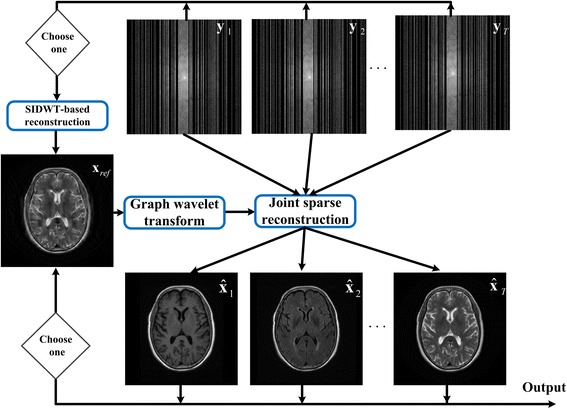
Flowchart of the proposed method. The x_ref denotes the reference image used to train the graph wavelet transform, y₁, y₂, ⋯, y_T denote the under-sampled k-space data of multi-contrast images, ${\widehat{\mathbf{x}}}_1,{\widehat{\mathbf{x}}}_2,\cdots ,{\widehat{\mathbf{x}}}_T$ denote the reconstructed images

Graph-based redundant wavelet transform

Given a reference image, the GBRWT is achieved by carrying out redundant wavelet transform on permuted signals of new orders [7]. The new orders are found in weighted graph constructed from the reference image, in which image patches collected by a sliding window serve as the vertex and the patch similarities computed using w_{m, n} = w(b_m, b_n) = ‖b_m − b_n‖₂ (where b_m and b_n denote the m^th and the n^th patches) serve as the weight. The new orders are obtained by finding the shortest possible path on the patch-based graph [7, 20]. Then, redundant wavelet transform is performed on permuted pixels to achieve sparse representation.

The process of permutation and wavelet filtering in GBRWT is shown in Fig. 2. In the l^th level decomposition, the input signal a_l will be first reordered by permutation matrix P_l, whose inverse process is ${\mathbf{P}}_l^{\mathrm{H}}$ and satisfied ${\mathbf{P}}_l^{\mathrm{H}}{\mathbf{P}}_l=\mathbf{I}$. Then, non-decimated wavelet transformation Φ_l, whose inverse process is ${\mathbf{\Phi }}_l^{\mathrm{H}}$ and satisfied ${\mathbf{\Phi }}_l^{\mathrm{H}}{\mathbf{\Phi }}_l=\mathbf{I}$, are performed on the re-ordered pixels. The output a_l + 1 and d_l + 1 of l^th level non-decimated decomposition will be of the same size with the input signal ${\tilde{a}}_l$. Let Φ_lP_l be the l^th level decomposition of GBRWT, and ${\mathbf{P}}_l^{\mathrm{H}}{\mathbf{\Phi }}_l^{\mathrm{H}}$ be corresponding composition process, and then Φ_lP_l satisfies the following property

$${\mathbf{P}}_l^{\mathrm{H}}{\mathbf{\Phi }}_l^{\mathrm{H}}{\mathbf{\Phi }}_l{\mathbf{P}}_l=c\mathbf{I},$$ 3

where c denotes the redundancy of GBRWT transform. It has been verified that GBRWT provides sparser representations than traditional wavelet transform, thus can improve the MRI image reconstruction [7].

Fig. 2.

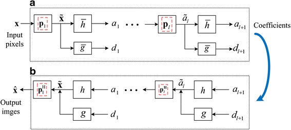
The permutation and wavelet filtering on re-ordered image pixels, a and b are the forward and inverse transforms

Joint sparsity of multi-contrast image coefficients

Multi-contrast MRI images are obtained by different parameter settings, but share the same anatomical cross section [6–8]. The image structures corresponding to tissue locations remain unchanged with contrast varied, which leads to spatial position-related coefficients. Joint sparsity means that, under appropriate sparsifying transforms, the positions of non-zero coefficients correspond directly to same spatial locations in multiple images. Figure 3 shows that the non-zero transform coefficients of two contrast images occur at the same positions in the Haar wavelets transform and GBRWT domains. Thus, the joint sparsity of GBRWT provides extra information on images and may further improve the reconstruction of multi-contrast images.

Fig. 3.

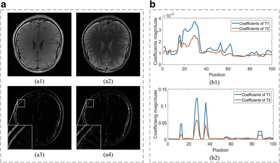
Joint sparsity property of multi-contrast image coefficients. Group sparsity for traditional wavelet transform is shown in (A), (a1-a4) are images of two contrasts (T1W and T2W MRI images) and their corresponding coefficients in the 3rd sub-bands of traditional redundant Haar wavelet transform. Group sparsity of GBRWT is shown in (B) and (b1-b2) are two selected fragments of GBRWT coefficients

Problem formulation

The joint sparsity promoting problem in multi-contrast MRI image reconstruction with GBRWT is solved using the mixed ℓ_{2, 1} norm minimization [9, 21, 22]:

$$\underset{\mathbf{x}}{min}{‖\mathbf{G\Psi x}‖}_{2,1}s.t.{‖\mathbf{UFx}-\mathbf{y}‖}_2^2\le {\sigma }^2,$$ 4

where, $\mathbf{\Psi }=\left[\begin{array}{ccc}{\mathbf{\Psi }}_g& 0& 0\\ 0& \ddots & 0\\ 0& 0& {\mathbf{\Psi }}_g\end{array}\right]$ and Ψ_g denotes the GBRWT representation, in which l^th level decomposition be expressed as Φ_lP_l. Let α = Ψx be the corresponding coefficients, then for an image set which includes T kinds of contrasts, the column stacked coefficients can be expressed as: α = [α₁; ⋯; α_T]. The role of grouping operator G is to reshape the column stacked coefficients of multi-contrast MRI images into a matrix as shown in Fig. 4. Then, one column of Gα stands for coefficients of one image, and one row forms a group.

Fig. 4.

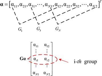
The grouping operator G and the grouped GBRWT coefficients

The ℓ_{2, 1} norm is defined as

$${‖\mathbf{G\alpha }‖}_{2,1}=\sum _{i=1}^N{\left(\sum _{j=1}^T{\left|{\mathbf{\alpha }}_{\mathit{ij}}\right|}^2\right)}^{1/2},$$ 5

where, G is the group operator, N is the number of transform coefficient and T the number of contrast.

Numerical algorithm

The alternating direction method with continuation [18] is incorporated in the ℓ_{2, 1} norm optimization. Let α = Ψx, the objective in Eq. (4) can be rewritten as

$$\underset{\mathbf{x},\mathbf{\alpha }}{min}{‖\mathbf{G\alpha }‖}_{2,1}\begin{array}{cc}\begin{array}{cc}& s.t.\end{array}& {‖\mathbf{UFx}-\mathbf{y}‖}_2^2\le {\sigma }^2,\mathbf{\alpha }=\mathbf{\Psi x}\end{array}.$$ 6

Furthermore, the objective function in (6) can be over-relaxed to be unconstraint as

$$\underset{\mathbf{x},\mathbf{\alpha }}{min}{‖\mathbf{G\alpha }‖}_{2,1}+\frac{\beta }{2}{‖\mathbf{\alpha }-\mathbf{\Psi x}‖}_2^2+\frac{\lambda }{2}{‖\mathbf{UFx}-\mathbf{y}‖}_2^2.$$ 7

The λ is a parameter to balance the sparsity and data fidelity. The β is fixed in the inner loops and changes continuously to achieve optimal reconstruction in the outer loops. When β → ∞, the solution of Eq. (7) approaches to that of Eq. (6). When β is fixed, x and α will be computed alternatively by the following two steps:

1. With x fixed, α will be computed by solve the objective:

$$\underset{\mathbf{\alpha }}{min}{‖\mathbf{G\alpha }‖}_{2,1}+\frac{\beta }{2}{‖\mathbf{\alpha }-\mathbf{\Psi x}‖}_2^2.$$ 8

Algorithm 1: Joint multi-contrast MRI reconstruction based on GBRWT

Parameters: λ Input:

k-space data y = [y1; ⋯; yT]; g levels of permutation orders Pj,  {j = 1, ⋯, g}; regularization parameter λ; tolerance of inner loop η = 10−4.

Initialization: x = (UF)Hy, xprevious = x, β = 26.

Main:

While β ≤ 212

(1) Given x, solving α by computing Eq. (10) for each group of coefficients αi,  {i = 1, ⋯, N};

(2) Applying α into Eq. (12) to obtain the solution x; (3) If ‖Δx‖ = ‖xprevious − x‖ > η, then xprevious = x, go to step (1); Otherwise: go to step (4); (4) $\widehat{\mathbf{x}}\mathbf{=}\mathbf{x}$, β = 2β, go to step (1);

End while

Output $\widehat{\mathbf{x}}$

To find the extreme of objective function in Eq. (8), firstly the equivalent transformation ${‖\mathbf{\alpha }-\mathbf{\Psi x}‖}_2^2={‖\mathbf{G\alpha }-\mathbf{G}\left(\mathbf{\Psi x}\right)‖}_F^2$ is taken; then, the coefficients in rows of Gα (each group) are computed separately by solving least square method. Let αⁱ = (Gα)_{i, :}, (Ψx)ⁱ = (Ψx)_{i, :} denote the ith group of Gα and Ψx respectively, we find solution by

$$\underset{{\mathbf{\alpha }}^i}{min}{‖{\mathbf{\alpha }}^i‖}_2+\frac{\beta }{2}{‖{\mathbf{\alpha }}^i-{\left(\mathbf{\Psi x}\right)}^i‖}_2^2.$$ 9

Then, α can be obtained via each group computing:

$${\mathbf{\alpha }}^i=\left\{\begin{array}{c}\frac{{‖{\left(\mathbf{\Psi x}\right)}^i‖}_2-\frac{1}{\beta }}{{‖{\left(\mathbf{\Psi x}\right)}^i‖}_2}{\left(\mathbf{\Psi x}\right)}^i,{‖{\left(\mathbf{\Psi x}\right)}^i‖}_2>\frac{1}{\beta }\\ \begin{array}{cccc}& & 0& \begin{array}{cc}\begin{array}{cc}& \begin{array}{cc}& ,\end{array}\end{array}& {‖{\left(\mathbf{\Psi x}\right)}^i‖}_2\le \frac{1}{\beta }\end{array}\end{array}\end{array}\right..$$ 10

• 2)Fix α, x can be computed by solving

$$\underset{\mathbf{x}}{min}\beta {‖\mathbf{\alpha }-\mathbf{\Psi x}‖}_2^2+\lambda {‖\mathbf{UFx}-\mathbf{y}‖}_2^2.$$ 11

The minimization with respect to x can be solved by finding the extreme of least square problem in Eq. (11). Finally, we get

$$\mathbf{x}={\mathbf{F}}^{\mathrm{H}}{\left(\mathit{\beta c}\mathbf{I}+\lambda {\mathbf{U}}^{\mathrm{H}}\mathbf{U}\right)}^{-1}\left(\beta {\mathbf{F\Psi }}^{\mathrm{H}}\mathbf{\alpha }+\lambda {\mathbf{U}}^{\mathrm{H}}\mathbf{y}\right),$$ 12

where, c is the redundancy caused by GBRWT transform. The numerical algorithm pseudo-code is listed in Algorithm 1.

Results

The image reconstruction was performed on a server with E5-2637 v3 (3.5G Hz) *2 CPU, 8 GB memory. The proposed method, Joint sparse reconstruction based on GBRWT (JGBRWT), is compared with the Joint sparse reconstruction method based on SIDWT (JSIDWT) [15–17], that replacing Ψ_g with SIDWT in Eq. (4) and Joint reconstruction with Bayesian Compressed Sensing (JBCS) [19], which is a state-of-the-art joint multi-contrast image reconstruction that jointly explores the gradient coefficients of multiple images. The comparison with GBRWT-based single image reconstruction [7] is also included to demonstrate the advantage of the joint reconstruction. The parameter values for JBCS are taken as the same in the cods shared by the authors (http://martinos.org/~berkin/software.html). For the proposed method and JSIDWT, λ is set as 10⁴.

The relative ℓ₂ norm error (RLNE) defined as $e\left(\stackrel{⌢}{\mathbf{x}}\right)\mathbf{=}{‖\stackrel{⌢}{\mathbf{x}}\mathbf{-}\tilde{\mathbf{x}}‖}_{\mathbf{2}}/{‖\tilde{\mathbf{x}}‖}_{\mathbf{2}}$ (in which $\tilde{\mathbf{x}}$ is ground truth and $\stackrel{⌢}{\mathbf{x}}$ is the reconstructed image) and mean structure similarity index measure (MSSIM) [23] served as the criteria for assessing the quality of reconstructed image quality. Smaller RLNE means lower reconstructed error and higher MSSIM indicates better structure preservation capability.

The Brainweb images (http://brainweb.bic.mni.mcgill.ca/) [24, 25] (Fig. 5) as well as the in vivo multi-contrast images were used to validate the efficiency of the proposed method. The multi-contrast knee images (Fig. 6) were acquired from GE 3 Tesla scanner (Discovery MR750W, USA) with parameters (T1W: FSE, TR/TE = 499 ms/9.63 ms; T2W: TR/TE = 2435 ms/49.98 ms, Proton density weighted image: TR/TE = 2253 ms/31.81 ms; FOV = 180 × 180 mm², slice thickness = 4 mm). The multi-contrast brain images (Fig. 7) were acquired from SIMENS 3 Tesla scanner (MAGNETOM Trio Tim, Germany) with parameters (T2W: TSE, TR/TE = 3000 ms/66 ms,; T1W, FLAIR: TR/TE = 3900 ms/9.3 ms,; FOV = 200 × 200 mm², slice thickness = 5 mm) for Fig. 7(A) and TSE: TR = 4000 ms, FOV = 192 × 192 mm², slice thickness = 3 mm, ∆TE =8 ms for the multi-echo data in Fig. 7(B).

Fig. 5.

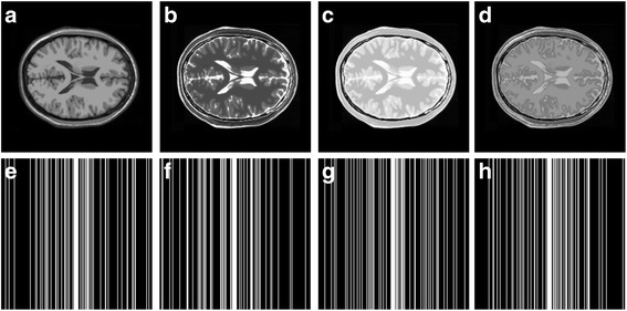
Multi-contrast Brainweb image reconstruction. a-d images with four contrasts; e-h sampling patterns operated on individual contrast images at the same sampling rate 22%

Fig. 6.

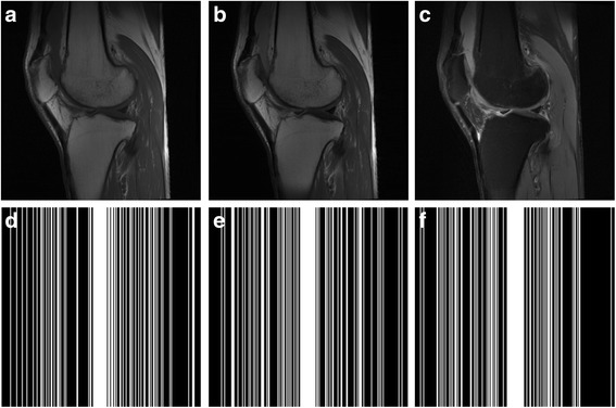
Multi-contrast knee images and under-sampling masks. a-c multi-contrast knee images with 3 kinds of contrasts; d-f 3 different sampling masks operating on each image of individual contrast with the same sampling rate 32%

Fig. 7.

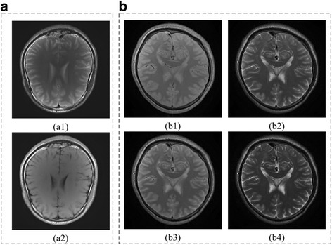
Multi-contrast brain MRI images. (A) are T2W and T1W images of one subject; (B) are images with 4 kinds of contrast for another subject by setting TE to different values

Fully sampled multi-contrast MRI images shown in Figs 5, 6 and 7 are used for the experiment of under-sampling and joint sparse reconstruction. Reconstruction errors shown in Figs. 8, 9 and 10 reveal that the proposed method outperforms the JSIDWT and JBCS. The lower error of the proposed method indicates better fidelity and edge-preserving capabilities compared with JSIDWT and JBCS. Besides, the reconstruction errors were reduced when comparing the proposed method with single image reconstruction based on the same GBRWT transform, implying that the improvement obtained by joint reconstruction over single image reconstruction.

Fig. 8.

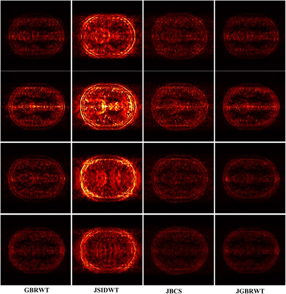
Brainweb reconstruction errors (× 5) with 22% sampled data (Cartesian). Rows 1–4 correspond to multi-contrast images shown in Fig. 5 (a-d) respectively. Columns 1–4 denote the results obtained from individual reconstruction based on GBRWT, JSIDWT, JBCS and JGBRWT reconstruction respectively

Fig. 9.

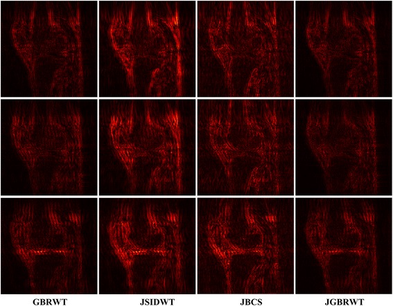
Reconstruction errors of knee images (_× 5) with 32% sampled data (Cartesian). Rows 1–3 correspond to multi-contrast images shown in Fig. 6(a-c) respectively. Column 1–4 denote the results obtained from GBRWT, JSIDWT, JBCS and JGBRWT reconstruction respectively

Fig. 10.

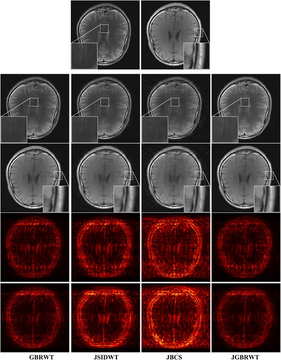
Reconstructed brain images and corresponding errors (_× 5) with 27% sampled data. The 1st row shows fully sampled multi-contrast images, the 2nd and 3rd rows are reconstructed images and last two rows are reconstruction errors corresponding to the 2nd and 3rd rows, respectively. Columns 1 to 4 denote the results obtained from GBRWT, JSIDWT, JBCS and JGBRWT, respectively

Tables 1, 2 and 3 show RLNEs and MSSIMs of reconstructed images. These criteria indicate that the proposed method gained the highest MSSIM and the lowest RLNE, and thus recovered the images most faithfully.

Table 1.

RLNE/MSSIM of Brainweb images with 22% Cartesian sampled data in Fig. 5

Images	GBRWT	JSIDWT	JBCS	JGBRWT
Fig. 5(a)	0.0688/0.9321	0.1643/0.6944	0.0985/0.7091	0.0365/0.9799
Fig. 5(b)	0.1048/0.9206	0.2284/0.6774	0.1336/0.7143	0.0609/0.9701
Fig. 5(c)	0.0492/0.9038	0.1233/0.6742	0.0525/0.7665	0.0232/0.9815
Fig. 5(d)	0.0660/0.9100	0.1222/0.7265	0.0596/0.8005	0.0306/0.9821

Table 2.

RLNE/MSSIM of knee images with 32% Cartesian sampled data in Fig. 6

Images	GBRWT	JSIDWT	JBCS	JGBRWT
Fig. 6(a)	0.0615/0.9560	0.0932/0.9211	0.0850/0.9064	0.0582/0.9624
Fig. 6(b)	0.0629/0.9605	0.0976/0.9234	0.0890/0.9004	0.0534/0.9704
Fig. 6(c)	0.0883/0.9337	0.1216/0.9312	0.1238/0.9180	0.0823/0.9607

Table 3.

RLNE/MSSIM of reconstructed brain images with 27% sampled data in Fig. 7

Images	GBRWT	JSIDWT	JBCS	JGBRWT
Fig. 7(a1)	0.0505/0.9612	0.0924/0.9089	0.1297/0.7759	0.0487/0.9636
Fig. 7(a2)	0.0762/0.9593	0.1103/0.9149	0.1502/0.7817	0.0733/0.9639

One typical brain image reconstruction with 27% sampled data are shown in Fig. 10. In the zoomed-in area of the 2nd row, the sulcus of the T2W image appears in the middle of the fully sampled and JGBRWT reconstructed images, but nearly disappears for JBCS reconstruction. In the marked region of the 3rd, the proposed method leads to more consistent reconstruction with the fully sampled image than other methods. These improvements are also confirmed by the error images in the last two rows.

2D under-sampling

The 2Dunder-sampling patterns (Fig. 11) was explored to demonstrate the potential applications of the proposed method in 3D imaging, in which 2D phase encoding plane can be under-sampled.

Fig. 11.

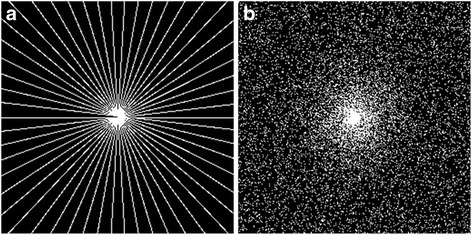
The 2D under-sampling mask. a is pseudo-radial sampling with sampling rate 11%, b is random sampling with sampling rate 15%

Brainweb reconstructed errors shown in Fig. 12 demonstrate that on the simulated database, the lowest reconstruction errors were obtained with the proposed method. The corresponding RLNE/MSSIM are shown in Table 4. Figure 13 implies that the proposed method led to the lowest brightness in the error images and thus maintained fidelity best. The criteria listed in Tables 4 and 5 indicate that the proposed method achieved the highest MSSIM and the lowest RLNE on the tested dataset.

Fig. 12.

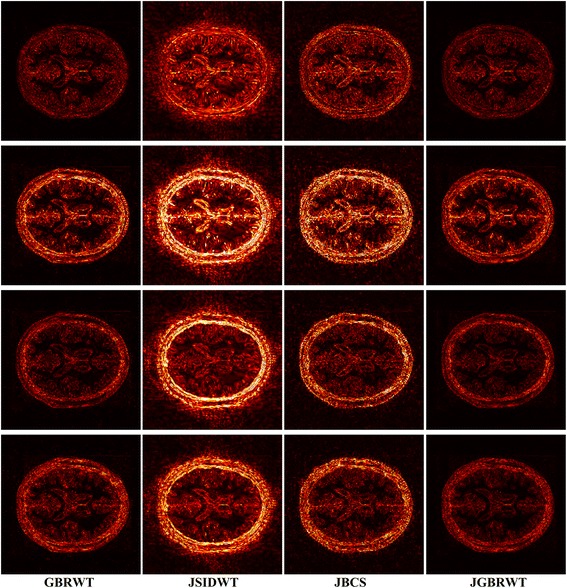
Reconstructed error (_× 5) using 2D pseudo-radial under-sampling with 11% sampled data of Fig. 5. Rows 1–4 correspond to multi-contrast images shown in Fig. 5 (a-d) respectively. Columns 1–4 denote the results obtained from GBRWT, JSIDWT, JBCS and JGBRWT reconstruction respectively

Table 4.

RLNE/MSSIM for the reconstruction using 11% pseudo-radial k-space data of Fig. 5

Images	GBRWT	JSIDWT	JBCS	JGBRWT
Fig. 5(a)	0.0443/0.9779	0.1011/0.6966	0.0835/0.8595	0.0395/0.9813
Fig. 5(b)	0.1036/0.9510	0.2118/0.6246	0.1632/0.7865	0.0811/0.9680
Fig. 5(c)	0.0327/0.9681	0.1008/0.6666	0.0663/0.8720	0.0304/0.9789
Fig. 5(d)	0.0606/0.9476	0.1206/0.7062	0.0890/0.8745	0.0444/0.9757

Fig. 13.

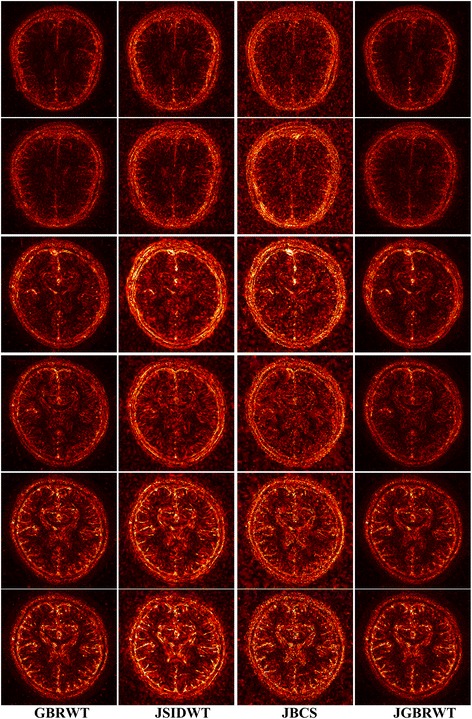
Reconstructed error (_× 5) using 2D Random under-sampling, with 15% sampled data in Fig. 7(a1-a2), and 26% sampled data in Fig. 7(b1-b4). Rows 1–6 are reconstruction errors correspond to multi-contrast images shown in Figs. 7(a1-a2, b1-b4) respectively. Columns 1–4 denote the results obtained from GBRWT, JSIDWT, JBCS and JGBRWT respectively

Table 5.

RLNE/MSSIM for the reconstruction using 15% randomly sampled k-space data of Fig. 7(A) and Fig. 7(B)

Images	GBRWT	JSIDWT	JBCS	JGBRWT
Fig. 7(a1)	0.0537/0.9526	0.0735/0.9222	0.0973/0.8220	0.0515/0.9562
Fig. 7(a2)	0.0735/0.9563	0.0957/0.9231	0.1097/0.8480	0.0722/0.9589
Fig. 7(b1)	0.0844/0.8820	0.1315/0.7739	0.1366/0.7129	0.0820/0.8955
Fig. 7(b2)	0.0935/0.8883	0.1278/0.8065	0.1302/0.7698	0.0817/0.9142
Fig. 7(b3)	0.1327/0.8611	0.1691/0.7821	0.1707/0.7411	0.1184/0.8876
Fig. 7(b4)	0.1624/0.8481	0.2158/0.7544	0.2054/0.7602	0.1558/0.8688

Different sampling rates

The curves in Fig. 14 show that the RLNEs decreased with sampling rate increased. The RLNE line of the proposed JGBRWT method (dark green line) is lower than that of GBRWT (or contrast-by-contrast reconstruction, black line) with the same GBRWT representation, indicating benefits are achieved by utilizing joint sparsity among multi-contrast images. The JGBRWT also outperforms other joint reconstruction method, including JSIDWT (red line) and JBCS (blue line), in terms of lower RLNEs at all sampling rates.

Fig. 14.

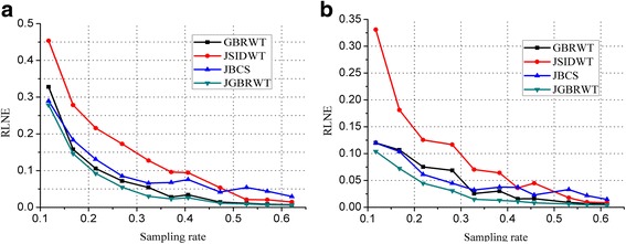
RLNEs evaluation at various sampling rates. a and b display the RLNEs with regard to the fully sampled data shown in Figs. 5(b) and (d) under Cartesian under-samplings

The same sampling patterns

The proposed method is compatible to same or different sampling patterns. Reconstruction criteria in Table 6 show that the proposed method outperforms the compared ones under the same sampling patterns. Besides, at the same sampling rate, using different sampling patterns lead to better evaluation criteria than using same sampling patterns (Table 6 vs. Table 1).

Table 6.

RLNE/MSSIMs under same sampling patterns (sampling rate 22%)

Images	GBRWT	JSIDWT	JBCS	JGBRWT
Fig. 5(a)	0.0705/0.9305	0.1683/0.6858	0.1019/0.7422	0.0420/0.9760
Fig. 5(b)	0.0986/0.9322	0.2308/0.6536	0.1362/0.7371	0.0696/0.9661
Fig. 5(c)	0.0412/0.9309	0.1340/0.6505	0.0540/0.7768	0.0248/0.9788
Fig. 5(d)	0.0563/0.9366	0.1382/0.7036	0.0635/0.8190	0.0331/0.9796

Discussions

Limitations on choosing image to train the graph

Choose an arbitrary pre-reconstructed image as reference will lead to reconstruction errors (RLNEs) slightly change as shown in Fig. 15. But the RLNEs are still much lower than single image reconstruction. A possible way in the future work is to train a GBRWT jointly from all the under-sampled multi-contrast images to make full use of the common/complementary information of multi-contrast images.

Fig. 15.

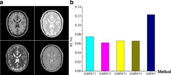
Effect of reference images. a multi-contrast images (contrast 1–4 are arranged from left to right, from top to bottom); b average reconstruction RLNEs of multi-contrast images in JGBRWT using different references and in GBRWT. Note: JGBRWT1 denote the JGBRWT using image of contrast 1 as reference, and so on

Limitations on un-registered images

Un-registered multi-contrast images will go against the joint sparsity assumption, and thus affect joint reconstruction performance. Reconstructed images of aligned and misaligned multi-contrast images (we simulate misalignment by rotating Fig. 16(a) with 10 degrees) shown in Fig. 16 demonstrate that misalignment will make the detail reconstruction deteriorated. RLNE obviously increased in sparse reconstruction of misaligned multi-contrast images. Improved image reconstruction is expected by incorporating the registration into image reconstruction process as it was done in [6], which would be interesting as a future work.

Fig. 16.

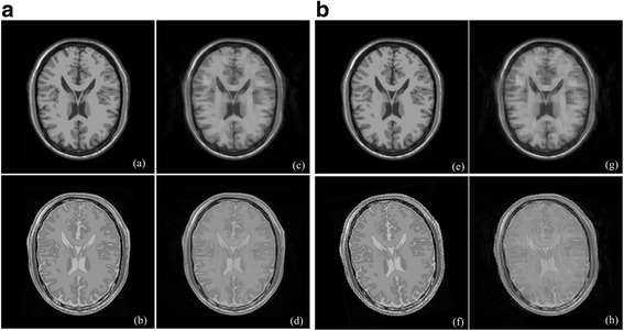
Joint sparse reconstruction with aligned and misaligned multi-contrast images at sampling rate 16%. (a)-(b) are aligned fully sampled images; (c)-(d) are reconstruction with RLNE = 0.1016 and RLNE = 0.0667, respectively; (e)-(f) are misaligned fully sampled images; (c)-(d) are reconstruction with RLNE = 0.1277 and RLNE = 0.1071, respectively

Computation complexity

The main step of numerical algorithm to solve the proposed joint reconstruction problem include a soft thresholding to solve α and a one-step computation to solve x, which is with the same computation complexity as single contrast image reconstruction, but with more data to compute, and thus no obvious additional computational burden.

Program at our platform (E5–2637 v3 (3.5G Hz) *2 CPU, 8 GB memory) shows that, the SIDWT-based single image reconstruction need 20 s, and SIDWT-based joint reconstruction need 100 with 4 different contrast images at low sampling rate. The GBRWT-based single image reconstruction need 200 s and GBRWT-based joint reconstruction need 103 s with 4 different contrast images at low sampling rate.

Experiment with noise

Multi-contrast images in Fig. 7(A) in the manuscript are used in noise experiment. Noisy data are simulated by adding Gaussian white noise with variance σ² = 0.02 on real and imaginary part of k-space data. Figure 17 demonstrate that the proposed method outperforms the compared ones in preserving image structures as well as removing noise. According to Table 7 the proposed method achieves lowest RLNEs, highest MSSIMs and highest SNRs. The signal to noise rate (SNR) is defined as SNR = 10log₁₀(μ/σ), where u is the mean of image density and δ is the standard deviation of the noise extracted from the image background.

Fig. 17.

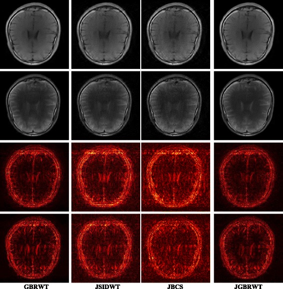
Noisy experiment (with 27% sampled data) under Gaussian white noise with variance σ² = 0.02. Rows 1–2: reconstructed images; Rows 3–4: magnitude errors (× 5)

Table 7.

SNR/MSSIM/RLNEs in noise experiment with 27% sampled data

Images	GBRWT	JSIDWT	JBCS	JGBRWT
Fig. 7(a1)	18.59/0.9108/0.0814	15.51/0.7977/0.1161	14.28/0.7168/0.1337	19.58/0.9247/0.0726
Fig. 7(a2)	15.74/0.9031/0.1179	14.10/0.7845/0.1424	12.94/0.7012/0.1627	16.61/0.8241/0.1067

Parameters

Two noise level are considered (Gaussian white noise with variance σ² = 0.02 and σ² = 0.03) in testing λ. The optimal λ for σ² = 0.02 and σ² = 0.03 are 600 and 400 respectively on the tested data according the curve shown in Fig. 18.

Fig. 18.

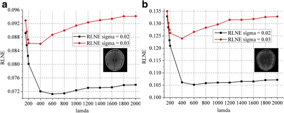
The optimal λ under different noise levels. a-b are RLNE curves for each contrast image. Note: Two contrast images under 1D under-sampling pattern at sampling rate 27% are reconstructed using the proposed JGBRWT

The parameters of GBRWT include patch-size and decomposition levels, which have been discussed in [7]. The suggested patch-size in GBRWT are from 4 × 4 to 7 × 7, and suggested decomposition level is 3–5 level. We use the patch-size 7 × 7 and do 5 level decomposition in this experiment.

Conclusions

A new approach is proposed to simultaneously explore the adaptive sparse image representation under graph-based redundant wavelet transform and the joint sparse reconstruction of multi-contrast MRI images. Experimental results in synthetic and in vivo MRI data demonstrate that the proposed method can achieve lower reconstruction errors than the compared methods. With this high quality image reconstruction method, it is possible to achieve the high acceleration factors by exploring the complementary information provided by multi-contrast MRI.

Abbreviations

ADMC

Alternating direction method with continuity

GBRWT

Graph-based redundant wavelet transform

JBCS

Joint reconstruction based on Bayesian compressed sensing

JGBRWT

Joint sparse reconstruction based on GBRWT

JSIDWT

Joint sparse reconstruction based on SIDWT

MRI

Magnetic resonance imaging

MSSIM

Mean structure similarity index measure

PDW

Proton density weighted MRI image

RLNE

Relative ℓ₂ norm error

SIDWT

Shift invariant discrete wavelet transform

T1W

T1 weighted MRI image

T2W

T2 weighted MRI image

Authors’ contributions

XQ designed the joint multi-contrast MRI reconstruction method and ZL implemented this method. Algorithm development and data analysis were carried out by ZL, XZ, DG, XD, YY, GG, ZC and XQ. All authors have been involved in drafting and revising the manuscript and approved the final version to be published. All authors read and approved the final manuscript.

Ethics approval and consent to participate

This study (joint reconstruction of knee images) was approved by Institutional Review Board of No.2 Hospital Xiamen (ethical approval number 2014001). This retrospective study (joint reconstruction of brain MRI images) was approved by Institute Review Board of Shenzhen Institutes of Advanced Technology, Chinese Academy of Science (ethical approval number SIAT-IRB-130315-H0024). Participant for all images have informed consent that he knew the risks and agreed to participate in the research.

Competing interests

One author, Xiaobo Qu, works as a Section Editor for the BMC Medical Imaging. The other authors declare that they have no competing interests.

Publisher’s Note

Springer Nature remains neutral with regard to jurisdictional claims in published maps and institutional affiliations.

References

- 1.Lustig M, Donoho DL, M. Santos J, Pauly JM. Compressed sensing MRI. IEEE Signal Process Mag. 2008;72:72–82. doi: 10.1109/MSP.2007.914728. [DOI] [Google Scholar]
- 2.Lustig M, Donoho D, Pauly JM. Sparse MRI: the application of compressed sensing for rapid MR imaging. Magn Reson Med. 2007;58(6):1182–1195. doi: 10.1002/mrm.21391. [DOI] [PubMed] [Google Scholar]
- 3.Li E, Khalvati F, Shafiee MJ, Haider MA, Wong A. Sparse reconstruction of compressive sensing MRI using cross-domain stochastically fully connected conditional random fields. BMC Med Imaging. 2016;16(1):51. doi: 10.1186/s12880-016-0156-6. [DOI] [PMC free article] [PubMed] [Google Scholar]
- 4.Yang BX, Yuan M, Ma YD, Zhang JW, Zhan K. Local sparsity enhanced compressed sensing magnetic resonance imaging in uniform discrete curvelet domain. BMC Med Imaging. 2015;15(1):28. doi: 10.1186/s12880-015-0065-0. [DOI] [PMC free article] [PubMed] [Google Scholar]
- 5.Liu Y, Zhan Z, Cai J-F, Guo D, Chen Z, Qu X. Projected iterative soft-thresholding algorithm for tight frames in compressed sensing magnetic resonance imaging. IEEE Trans Med Imaging. 2016;35:2130–2140. doi: 10.1109/TMI.2016.2550080. [DOI] [PubMed] [Google Scholar]
- 6.Lai Z, Qu X, Lu H, Peng X, Guo D, Yang Y, Guo G, Chen Z. Sparse MRI reconstruction using multi-contrast image guided graph representation. Magn Reson Imaging. 2017;43:95–104. doi: 10.1016/j.mri.2017.07.009. [DOI] [PubMed] [Google Scholar]
- 7.Lai Z, Qu X, Liu Y, Guo D, Ye J, Zhan Z, Chen Z. Image reconstruction of compressed sensing MRI using graph-based redundant wavelet transform. Med Image Anal. 2016;27:93–104. doi: 10.1016/j.media.2015.05.012. [DOI] [PubMed] [Google Scholar]
- 8.Huang J, Chen C, Axel L. Fast multi-contrast MRI reconstruction. Magn Reson Imaging. 2014;32(10):1344–1352. doi: 10.1016/j.mri.2014.08.025. [DOI] [PubMed] [Google Scholar]
- 9.Majumdar A, Ward RK. Joint reconstruction of multiecho MR images using correlated sparsity. Magn Reson Imaging. 2011;29(7):899–906. doi: 10.1016/j.mri.2011.03.008. [DOI] [PubMed] [Google Scholar]
- 10.Zheng H, Qu X, Bai Z, Liu Y, Guo D, Dong J, Peng X, Chen Z. Multi-contrast brain magnetic resonance image super-resolution using the local weight similarity. BMC Med Imaging. 2017;17(1):6. doi: 10.1186/s12880-016-0176-2. [DOI] [PMC free article] [PubMed] [Google Scholar]
- 11.Peng X, Ying L, Liu Y, Yuan J, Liu X, Liang D. Accelerated exponential parameterization of T2 relaxation with model-driven low rank and sparsity priors (MORASA) Magn Reson Med. 2016;76(6):1865–1878. doi: 10.1002/mrm.26083. [DOI] [PubMed] [Google Scholar]
- 12.Harmouche R, Cheriet F, Labelle H, Dansereau J. Multimodal image registration of the scoliotic torso for surgical planning. BMC Med Imaging. 2013;13(1):1. doi: 10.1186/1471-2342-13-1. [DOI] [PMC free article] [PubMed] [Google Scholar]
- 13.Zhan Z, Cai JF, Guo D, Liu Y, Chen Z, Qu X. Fast multiclass dictionaries learning with geometrical directions in MRI reconstruction. IEEE Trans Biomed Eng. 2016;63(9):1850–1861. doi: 10.1109/TBME.2015.2503756. [DOI] [PubMed] [Google Scholar]
- 14.Ravishankar S, Bresler Y. MR image reconstruction from highly undersampled k-space fata by dictionary learning. IEEE Trans Med Imaging. 2011;30(5):1028–1041. doi: 10.1109/TMI.2010.2090538. [DOI] [PubMed] [Google Scholar]
- 15.Qu X, Hou Y, Lam F, Guo D, Zhong J, Chen Z. Magnetic resonance image reconstruction from undersampled measurements using a patch-based nonlocal operator. Med Image Anal. 2014;18(6):843–856. doi: 10.1016/j.media.2013.09.007. [DOI] [PubMed] [Google Scholar]
- 16.Qu X, Guo D, Ning B, Hou Y, Lin Y, Cai S, Chen Z. Undersampled MRI reconstruction with patch-based directional wavelets. Magn Reson Imaging. 2012;30(7):964–977. doi: 10.1016/j.mri.2012.02.019. [DOI] [PubMed] [Google Scholar]
- 17.Baker CA, King K, Dong L, Leslie Y: Translational-invariant dictionaries for compressed sensing in magnetic resonance imaging. In: IEEE International Symposium on Biomedical Imaging: from nano to macro: March 30–April 2 2011: 1602–1605.
- 18.Yang J, Zhang Y, Yin W. A fast alternating direction method for TVL1-L2 signal reconstruction from partial fourier data. IEEE J Selected Topics Signal Processing. 2010;4(2):288–297. doi: 10.1109/JSTSP.2010.2042333. [DOI] [Google Scholar]
- 19.Bilgic B, Goyal VK, Adalsteinsson E. Multi-contrast reconstruction with Bayesian compressed sensing. Magn Reson Med. 2011;66(6):1601–1615. doi: 10.1002/mrm.22956. [DOI] [PMC free article] [PubMed] [Google Scholar]
- 20.Ram I, Elad M, Cohen I. Image processing using smooth ordering of its patches. IEEE Trans Image Process. 2013;22(7):2764–2774. doi: 10.1109/TIP.2013.2257813. [DOI] [PubMed] [Google Scholar]
- 21.Huang J, Zhang T. The benefit of group sparsity. Ann Stat. 2010;38(4):1978–2004. doi: 10.1214/09-AOS778. [DOI] [Google Scholar]
- 22.Eldar YC, Kuppinger P, Bolcskei H. Block-sparse signals: uncertainty relations and efficient recovery. IEEE Trans Signal Process. 2010;58(6):3042–3054. doi: 10.1109/TSP.2010.2044837. [DOI] [Google Scholar]
- 23.Zhou W, Bovik AC, Sheikh HR, Simoncelli EP. Image quality assessment: from error visibility to structural similarity. IEEE Trans Image Process. 2004;13(4):600–612. doi: 10.1109/TIP.2003.819861. [DOI] [PubMed] [Google Scholar]
- 24.Kwan RK, Evans AC, Pike GB. MRI simulation-based evaluation of image-processing and classification methods. IEEE Trans Med Imaging. 1999;18(11):1085–1097. doi: 10.1109/42.816072. [DOI] [PubMed] [Google Scholar]
- 25.Collins DL, Zijdenbos AP, Kollokian V, Sled JG, Kabani NJ, Holmes CJ, Evans AC. Design and construction of a realistic digital brain phantom. IEEE Trans Med Imaging. 1998;17(3):463–468. doi: 10.1109/42.712135. [DOI] [PubMed] [Google Scholar]
Associated Data
This section collects any data citations, data availability statements, or supplementary materials included in this article.
Data Availability Statement
The datasets used in the study will be publicly available at the authors’ website (http://csrc.xmu.edu.cn/project/GraphWavelet_JointSparseMRI/Toolbox_GraphWavelet_JointSparseMRI.zip).