

Abstract
This work formulates frictionless contact between solid bodies in terms of a repulsive potential energy term and illustrates how numerical integration of the resulting forces is computationally similar to the “pinball algorithm” proposed and studied by Belytschko and collaborators in the 1990s. We thereby arrive at a numerical approach that has both the theoretical advantages of a potential-based formulation and the algorithmic simplicity, computational efficiency, and geometrical versatility of pinball contact. The singular nature of the contact potential requires a specialized nonlinear solver and an adaptive time stepping scheme to ensure reliable convergence of implicit dynamic calculations. We illustrate the effectiveness of this numerical method by simulating several benchmark problems and the structural mechanics of the right atrioventricular (tricuspid) heart valve. Atrioventricular valve closure involves contact between every combination of shell surfaces, edges of shells, and cables, but our formulation handles all contact scenarios in a unified manner. We take advantage of this versatility to demonstrate the effects of chordal rupture on tricuspid valve coaptation behavior.
Keywords: Heart valves, Contact problems, Pinball algorithm, Isogeometric analysis
1. Introduction
The atrioventricular heart valves (i.e., the mitral and tricuspid valves) are structures in the heart that permit blood flow from the atria into the ventricles during diastole, as the heart relaxes. They then block blood from being pumped back out when the heart contracts, during systole. The semilunar valves (i.e., the aortic and pulmonary valves) play the opposite role, permitting blood to be pumped out of the ventricles, into the aorta and pulmonary artery, during systole, and preventing backflow into the ventricles during diastole.
The semilunar valves function in a relatively simple way: each one consists of three (or occasionally two) cup-like leaflets (cusps), attached to the sides of its respective artery. The convex sides of the leaflets face the ventricles, so that the leaflets fill up in reaction to backflow. When this happens, the convex sides of the leaflets contact one another, blocking flow. The mechanism of the atrioventricular valves is much more complicated. They are generally considered to have several distinct leaflets, but, in reality, these leaflets form contiguous sheets of tissue. These contiguous structures crumple up against themselves during systole to block off the channels between the ventricles and the atria. In as much as 3% of the human population [1], parts of an atrioventricular valve may even prolapse into the atrium. The atrioventricular valves’ mechanics are further complicated by a web-like network of tendons—the chordae tendineae, or “heart strings”—which tether the leaflets to the inside of the ventricles.
Computer simulations of the mechanics of heart valves play an increasingly important role in research into treatments for valvular heart disease. The need for and history of such simulations are reviewed in [2, 3]. As one might imagine, the treatment of contact mechanics is a major concern in these computations and proves to be especially difficult in the case of atrioventricular valves. Our previous work on aortic valve simulations [4–7] pointed out that to “avoid stagnation in pathological configurations, we typically select the resolution of the nonlinear algebraic solution by choosing a fixed number of iterations rather than a percentage by which the residual must be reduced” [4, page 1028]. Subsequent autopsies of poorly-converged steps indicated that contact forces were to blame for these “pathological configurations”.
Similar disclaimers can be found in other literature on aortic valve analysis. For example, to ensure completion of forward solves in an inverse modeling procedure, Aggarwal and Sacks [8] adhered to the following policy for terminating augmented Lagrangian iteration for contact: “After 10 augment iterations, the solution at current load was assumed to be converged irrespective of the gap and Lagrange multiplier values, and simulation was continued onto the next time step” [8, page 917]. It is clear that simulation of even the relatively simple contact of the aortic valve is fraught with difficulties. This has led some authors to instead apply brute-force explicit solution procedures that do not require solving a nonlinear algebraic problem at each step. However, Morganti et al. [9] reported that converging an explicit computation to a qualitatively-accurate configuration of a closed valve using standard finite elements in the thoroughly-optimized commercial code LS-DYNA [10] required more than 550 hours [9, Table 2] (i.e., more than 20 days). While the cited study indicates that using LS-DYNA’s isogeometric analysis capabilities in place of finite elements provided enormous improvements over that figure, the coarsest isogeometric computation still required a time step of 2.3 × 10⁻⁷ s [9, Table 2], which is several orders of magnitude smaller than the time step used for fluid–structure interaction (FSI) simulations in [4].
In light of these difficulties with aortic valve simulations, the outlook appears bleak for properly-converged implicit simulation of the more complicated atrioventricular valves, especially if one intends to study pathological configurations, such as prolapse, or incorporate FSI. Some example analyses of normal mitral valve structural mechanics using ABAQUS [11] can be found in [12–14]. Lee et al. [13, Section 10.4.3] indicate that “implicit dynamic analysis with automatic time stepping” was feasible in some cases, but the same authors note in [14, Section 2.6] that explicit dynamics using a time step of 10−6 s and mass scaling (as only the quasi-static limit was of interest) proved to be “a more general computational framework for future extensions, such as in vivo modeling and surgical simulations” [14, page 1287]. It is our experience that, even with the best commercial off-the-shelf software, some degree of case-by-case troubleshooting is frequently needed to solve complex contact problems using implicit methods. In the case of atrioventricular valve analysis, preprocessing and troubleshooting labor may be magnified by the involvement of contact between different combinations of 2D surfaces (leaflets) and 1D curves (representing the chordae tendineae and/or the edges of leaflets). Analysis methods that treat these different contact scenarios as separate cases are not only difficult to implement, but also often require additional pre-processing effort by the end user, to identify contact surfaces and curves, specify types of contact, and set a variety of options for each case (often by trial-and-error).
To approach the challenging problem of atrioventricular valve dynamics in a way that can be directly combined with the fluid–structure interaction (FSI) analysis methods of [4–7], which treat structural mechanics implicitly, we develop a novel contact formulation that builds on the concept of using repulsive forces that derive from a potential, as studied by Sauer and De Lorenzis [15]. We modify this framework to use volume rather than surface potentials, which can be applied to lower-dimensional objects (e.g., shells or cables) by multiplying surface or contour integrals over those objects with factors of thickness or cross-sectional area. This eliminates the need for special cases to handle contacts between objects of different co-dimensions to physical space. We discretize the integrals to compute contact potential energy using direct numerical quadrature (as applied to the case of electrostatic repulsion in [15, Section 5.3]), resulting in an n-body problem to determine contact forces. In general, this would require a Barnes–Hut [16] or fast multipole [17] approximation for computational efficiency. However, we simplify the n-body problem by using a compactly-supported potential with a limited range, so that each quadrature point interacts with only a handful of neighbors1 The geometry of the contacting bodies is thus approximated by a union of spherical potential supports, intersections of which are penalized in the potential energy functional for the system. The resulting discrete problem is similar in structure to that solved by the “pinball algorithm” proposed in Belytschko and Neal [20], but we use a different penalty function to apply forces to intersecting pinballs (i.e., supports of potential functions centered at quadrature points). Another related approach to contact was developed earlier by Sauer [21], motivated by coarse-graining of inter-atomic potentials, but, in the present work, we do not attempt to derive contact forces from any more basic physical principles; our choice of penalty function is motivated by calculations indicating the minimal level of singularity needed to prevent intersection of contacting bodies. We find that this potential-based contact formulation, combined with a specialized globalization strategy for nonlinear solution using Newton’s method and an adaptive time stepping technique, provides a reliable way to solve complicated contact problems with shell and cable structures, including atrioventricular valve dynamics.
The remainder of this paper is structured as follows. The formulation of the contact potential energy is detailed in Section 2, and its implementation using numerical quadrature is discussed in Section 3. The generic structural dynamics problem used for exposition in these sections is then specialized to the dynamics of a thin shell coupled to cables in Section 4. The contact formulation is tested in the context of this problem using several benchmarks. The right atrioventricular (i.e., tricuspid) valve is then modeled as an instance of this thin shell and cable problem in Section 5. Both normal and pathological tricuspid valve dynamics are successfully simulated. Section 6 summarizes our findings and discusses several other possible applications and extensions of the developed techniques.
2. Volume potentials for contact
To treat contact between objects of various co-dimensions to physical space, we first consider the case of solid bodies of co-dimension zero, then scale by factors of thickness and cross-sectional area to adapt the theory to thin shells of co-dimension one and cables of co-dimension two. We adopt this approach, in contrast to the surface potential framework of Sauer and De Lorenzis [15], for maximal geometric versatility. While the use of a surface potential allows for analytical simplification in the case of smooth surfaces [15, Appendix A], it requires additional information about the surface geometry. Formulation in terms of a volume potential permits contact to be modeled between objects represented by clouds of quadrature points, requiring no special treatment for contact between structures of arbitrary co-dimensions, with corners, edges, and other features that would complicate traditional contact algorithms. Further, volume potential based contact is compatible with meshfree discretizations that allow new surfaces to emerge spontaneously, through material rupture (e.g., the semi-Lagrangian reproducing kernel particle method (RKPM) [22]). It might be construed as a disadvantage that volume potentials result in a thin layer of body forces, as opposed to a true surface traction, but this force field could easily be integrated in the direction orthogonal to the surface as a post-processing step if surface tractions are desired. Alternatively, for bodies with well-defined surface parameterizations and no possibility of rupture, contact surfaces could be treated like structures of co-dimension one, by introducing a thickness length scale.
For simplicity of exposition, we assume, initially, that contact occurs between two disjoint bodies. The extension to multiple bodies is straightforward. The extension to self-contact is formulated in Section 2.2. The contact potential energy of two bodies with reference configurations and is given by
| (1) |
where and
| (2) |
in which y is a displacement field defined over and for v ∈ ℝd and p ≥ 1. To allow objects of nonzero co-dimension to simultaneously contact other objects from any direction, we must strongly enforce non-penetration of objects. This requires that Ec → ∞ as the distance between and approaches zero.
Remark 1
This potential energy term models frictionless contact. The absence of frictional effects is clear, as the formulation does not introduce any dissipative mechanisms. For bodies with smooth boundaries, and with typical choices of ϕ, one expects the resulting contact forces to be approximately normal to the boundaries. A detailed explanation of how tangential force contributions cancel is provided by Sauer and De Lorenzis [15, Appendix A] for the case of surface potentials. The cited article also comments briefly on how potential-based contact can be extended to include friction.
Remark 2
Enforcement of a gap between objects may also be useful in conjunction with immersed discretization schemes, in which the motion of a Lagrangian solid is derived from a velocity field represented on an Eulerian background mesh, either directly (e.g., [23, 24]), or through the computation of some coupling traction (e.g., [4, 25]). For example, in the standard material point method [24], a single continuous Eulerian velocity field represents the structure’s motion, so sliding contact proves difficult unless material points from different parts of the structure are prevented from coming within a background mesh dependent distance of one another. In the setting of immersed FSI, Kadapa et al. [26] report that stable simulation of fluid–rigid-body interaction using an immersed approach based on Nitsche’s method requires that the rigid bodies maintain a background mesh dependent distance between one another. The enforcement of a gap between immersed representations of structural components may seem to be at odds with the oft-touted advantage of immersed discretizations in representing topology changes. However, if gap width is tuned to match the size of elements in the background discretization, then it is, by construction, insufficient to resolve any spurious flow of material. (Thus, in a strange twist of irony, the numerical methods most capable of representing topology change tend to require it the least strictly.)
2.1. Selection of a potential
For computational tractability, we require that potentials have a finite range. To enforce non-penetration, we also clearly need ϕ(r) → ∞ as r → 0. However, too weak a singularity might still permit interpenetration of objects. For instance, consider a finite-thickness slab of electrically-charged material (i.e., ϕ(r) ~ 1/r): a simple application of Gauss’s theorem shows that the resulting electric field perpendicular to the slab never diverges, so that another charged object might tunnel through this slab with a finite amount of work (cf. [15, Section 3, Example 11, Remark 1]). To determine a sufficient strength of singularity for ϕ, let us consider smooth (or, at small scales, essentially flat) surfaces of Ω1 and Ω2 in contact. Our goal in designing ϕ is for the total repulsive force in the normal direction acting on ω1 ⊂ Ω1, as illustrated in Figure 1, to diverge.
Figure 1.

Notation for the integral used to show that p ≥ 4 is sufficient for the z-component of force on ω1 to diverge.
Let us assume that, for r less than some 𝒪(1) length scale, the potential has the form
| (3) |
As mentioned above, the obvious inadequacy of electrostatic repulsion for contact modeling leads us to the assumption that p > 2. The z-component of the force on ω1 can be bounded from below as follows:
| (4) |
where the integration variables x and ξ have the axial and radial coordinates (r, z) and (ρ, ζ) respectively, as shown in Figure 1, and D and θ depend on the integration variables x and ξ via
| (5) |
and
| (6) |
This is only a lower bound because it neglects additional repulsive forces on x ∈ Ω1 due to Ω2 \ωx. Integrating first over ωx, we get
| (7) |
| (8) |
| (9) |
| (10) |
| (11) |
where Ci are (possibly non-constant) finite coefficients and terms whose precise values are not important to the question of whether or not Fz is infinite. Integrating next over ω1, we obtain
| (12) |
| (13) |
To ensure that this lower bound diverges, we need to take p ≥ 4. To have the desired asymptotic behavior in the limit of r12 → 0 while maintaining a smooth but compactly-supported force field, we propose to model contact with the following force–separation law:
| (14) |
where rin and rout are length scales governing the support of the potential function, and kc is a dimensional constant. As discussed above, we assume p ≥ 4, to enforce non-penetration. The scalars c1 and c2 are uniquely determined by smoothness and continuity constraints:
| (15) |
and
| (16) |
An instance of this force law is illustrated in Figure 2.
Figure 2.
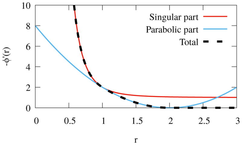
The function (14) with kc = 1, p = 4, rin = 1, and rout = 2.
As alluded previously, the extension of this concept to structures of nonzero co-dimension is accomplished by essentially performing one-point quadrature in the degenerated direction(s), to obtain surface, line, or point potentials, scaled by appropriate length, area, or volume factors. The conditions for non-penetration of potentials integrated on lower-dimensional geometries may be less severe. For instance, as shown in [15, Appendix A], the force field due to a less-singular 1/r2 potential integrated over a smooth surface is sufficient to produce divergent repulsive forces. The even milder electrostatic 1/r potential of an infinite line of charge can easily be shown, using Gauss’s theorem, to result in an electric field that diverges as one approaches the wire. However, these results are not robust for surfaces and curves with edges and endpoints, as often encountered in practical examples.
2.2. Extension to self-contact
In many cases of practical interest, there is no clear way to partition a structure into distinct parts that may contact one another; a body must be capable of contacting itself. To accomplish this, we consider all solid parts to be a single body with reference configuration Ω0 and modify the potential energy of contact to be
| (17) |
where BRself (X1) is the Euclidean ball of radius Rself around X1 and r12 is defined as before, but with both X1 and X2 in Ω0. The radius Rself must be selected in a problem-dependent way. It is clearly bounded below by the range of the contact potential, but, in general, must be somewhat larger, to prevent material compression from being identified as self-contact. If chosen too large, however, it might fail to identify some instances of self-contact.
3. Numerical implementation
In this section, we consider various aspects of implementing the proposed approach in finite element simulations. For simplicity, we consider a generic structural dynamics problem on the time interval (0, T). A specific example will be formulated in Section 5. The generic problem we consider in this section is: Find displacement y ∈ 𝒮y such that for all test functions z ∈ 𝒱y
| (18) |
where the forms B and F encapsulate the non-contact-related physics of the problem, 𝒮y and 𝒱y are displacement trial and test function spaces, and Dz is a functional derivative in direction z. Restricting y and z to yh and zh in finite-dimensional spaces and results in a finite element semi-discretization of the first term on the left-hand side of (18). We focus in this section on the discretization of the second term, which generates the contact forces.
We propose to compute the double integral in the definition of Ec numerically, using the same collection of quadrature points for each layer of integration. This results in a discrete Np-body problem:
| (19) |
where Np is the number of quadrature points,
| (20) |
| (21) |
Xi is the ith quadrature point and wi is its weight. The weights {wi} are assumed to include any additional length, area, or volume factors needed to convert surface, line, or point quadrature rules into volume quadrature. In this way, there is no difference in treatment between various co-dimensions of structural components when computing contact forces.
To ensure that the singular behavior is recovered as the distance between bodies shrinks all the way to zero, one would need to employ an adaptive quadrature rule; otherwise, a point from Ω2 could slip in between two points on the surface of Ω1 with a finite amount of work, making it possible for Ω2 to tunnel through Ω1, due to quadrature errors. Alternatively, one can prevent tunneling of objects through one another with a fixed quadrature rule by including an impenetrable core of infinite potential in the force–separation law. Consider the following modified force law:
| (22) |
where r = r12 − rmin and ϕ′ is as defined in (14). The support of the modified potential is of radius rmin + rout. (A procedure to avoid states of infinite energy during iterative nonlinear minimization of energy is given in Section 3.4.) If the zones of infinite potential about quadrature points in a body overlap, then the body is essentially impenetrable. For elastic bodies, tunneling is still technically possible, as adjacent points may be stretched apart, as illustrated schematically in Figure 3, but this would likely involve stresses well beyond the ultimate strength of most practical materials. We have nevertheless been able to produce this behavior by mashing objects together under displacement control. A similar concern is illustrated in [21, Figure 5.7].
Figure 3.
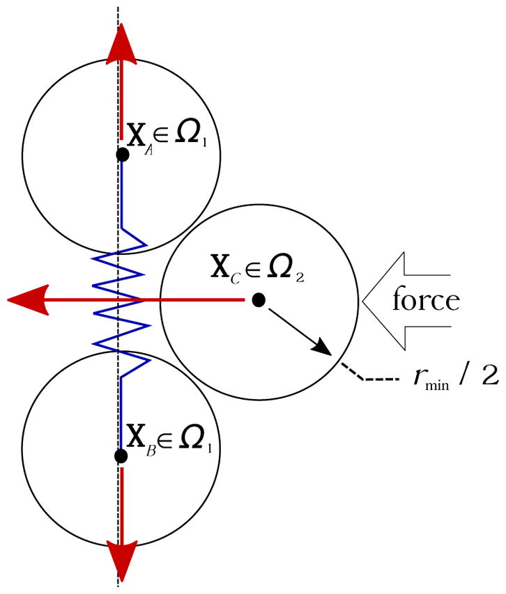
Suppose that quadrature points XA and XB from body Ω1 are constrained to slide along the dashed line and coupled by an elastic force, represented by the blue spring. Even with rmin > 0 and initially-overlapping regions of infinite penalty for points XA and XB, the contacting point XC from Ω2 can drive them apart if pushed with sufficient force.
3.1. Searching for interacting pairs of points
Due to the limited range of ϕ, the forces in the Np-body problem (19) can be evaluated efficiently. Assuming that the spatial number density of points is bounded below, there are only 𝒪(Np) nonzero terms in the double summation (19). We can avoid considering unnecessary pairs of points by sorting all of the quadrature points into the cells of a uniform grid, of cell size greater than or equal to the range rout + rmin of the potential. Then we only need to consider interactions between one point and others in the same or adjacent grid cells.
To describe the algorithm used precisely, we introduce some notation. Let the number of grid cells be Nc. These cells are a collection of disjoint subsets of ℝd denoted and cover the entire deformed configuration of the solid. The locations of the quadrature points in the current configuration are . We assume, as is especially true in the case of structures with nonzero co-dimension, that, while Nc may be very large, the vast majority of these grid cells are unoccupied at any given time. Thus operations of cost Θ(Nc)2 (such as iterating over all elements of {ωi}) should be avoided. Aside from allocating memory for the grid cells while initializing the data structure, operations to re-sort the points {xi} into new cells as the structure deforms should only iterate over occupied cells, of which there can be at most Np. Operations of cost Θ(Np) are necessarily acceptable; otherwise, it would be impossible to apply the contact forces, regardless of how they are computed.
We now introduce the necessary data structures for our algorithm:
L is an array of Np integers. This will be used to store linked lists of indexes of quadrature points. Because points fall within unique grid cells, these lists can all fit within a single array of size Np. The storage and traversal of these lists is clarified below.
S is a stack of integers. This is used to keep track of the indexes of occupied grid cells. S is initialized to be empty.
O is an array of Nc Boolean variables. O(i)3 indicates whether or not grid cell i is occupied. O is initialized to false once, when it is first allocated, costing Θ(Nc) operations.
H is an array of Nc integers. If O(i) is true, then H(i) indicates the head of a linked list of indexes of points from the set {xj} contained in grid cell ωi. The array H is initialized to zero once, when it is first allocated, costing Θ(Nc) operations.
The procedure for sorting elements of {xi} into grid cells {ωi} after the structure changes its configuration can be divided into two phases: purge the data structures of information about the previous configuration, then populate the data structures with information about the new configuration. The first phase, purging, is accomplished through the following steps:
Set the list L to zero. (Cost: Θ(Np), because L is of size Np.)
While S is not empty, pop index i from S, then set O(i) to false and H(i) to zero. (Cost: 𝒪(Np), because at most Np cells can be occupied by Np points, assuming each is in a unique cell.)
The second phase is accomplished by doing the following for each element xk of the set {xi}:
Identify the index i such that xk ∈ ωi. This can be accomplished in 𝒪(1) time, because the {ωj} are elements of a uniform grid.
If O(i) is false, set it to true and push i onto the stack S. (If O(i) is already true, do not redundantly push i.) This step also has cost 𝒪(1).
-
Update the linked list of points within this cell:
Store the old head of the linked list: h0 ← H(i).
Set xk’s index as the new head: H(i) ← k.
Connect the new head to the linked list: L(k) ← h0.
These steps cost 𝒪(1) time.
The cost of updating the data structures to reflect a change in the configuration of the structure is therefore Θ(Np). Once the data structures have been populated by the above algorithm, the list of points from {xj} contained in an occupied cell ωi can be traversed by looking at the point xi1, where i1 = H(i), then looking at xi2, where i2 = L(i1), and so on, until L(in) = 0, indicating the end of the list.4 If we assume that the points {xi} are distributed such that the number falling within any cell is 𝒪(1), then the cost of computing forces between all points in a cell and any adjacent occupied cells is 𝒪(1).
Remark 3
If the memory cost of storing H and O is prohibitive, random subsets of {ωi} can be mapped to bins of a hash table, through some nontrivial hash function mapping the cell index range {1, …, Nc} onto a smaller range {1, …, NH}, with NH < Nc. However, increasing the load factor (Np/NH) in this way comes at the cost of possibly computing moderately more zero forces between out-of-range pairs of points. We have not found it necessary to use hash functions other than the identity map in our computations, as memory was never a limiting factor.
3.2. Comparison with the pinball algorithm
As mentioned in Section 1, the fully-discrete penalization energy (19) can be construed as a variant of the pinball algorithm proposed by Belytschko and Neal in [20]. The idea of the pinball approach is to approximate the geometry of a structure by a collection of balls, referred to as “pinballs”, for the purposes of collision detection. Overlap of pinballs from different contacting bodies is then penalized, to prevent structures from intersecting one another. A refinement of this approach by Belytschko and Yeh, called the “splitting pinball method” [28, 29], tested for collisions using a hierarchical approach, such that, if two pinballs are detected as overlapping, each of them is split into a collection of finer pinballs (which may themselves be split, and so on, up to some user-defined recursion depth), to better approximate the underlying structural geometry.
Despite its simplicity and intuitive appeal, the pinball method remains relatively obscure today. It is, however, implemented in several actively-maintained production codes for explicit dynamics, such as EUROPLEXUS [30] and LS-DYNA [10]. According to the LS-DYNA manual [31], the original pinball method is “not recommended and is included only for back compatibility” [31, page 11–64], but the splitting variant [28, 29], added fairly recently in LS-DYNA R7.1, “is recommended when modeling complex contacts” [31, page 11–65]. Approaches with some similar features to the pinball algorithm have been developed independently for use in meshfree methods, where it is natural to consider the structure geometry as a collection of spheres and use these spheres to detect collisions. An example of such a method would be the kernel contact approach proposed by Guan et al. [22, Section 4].
We may view each quadrature point in our discrete formulation as a pinball of radius (rout + rmin)/2. The original paper on the pinball method [20] includes a separate definition of the surface normal vector at each pinball, but, in the later splitting approach, “The penalty force is always exerted in the direction between pinball centers, which enables the method to handle edge-to-surface, surface-to-surface and edge-to-edge contact” [29, page 382], which is more similar to what is done in the potential-based formulation of this paper. If we reinterpret the pinball approach as a quadrature scheme for a distributed contact force, the splitting variant is essentially adaptive quadrature.
3.3. Linearization of pairwise interactions
The interaction energy of two quadrature points at material positions X1 and X2 (separated by more than Rself at time zero) can be written as
| (23) |
where the scalar C accounts for quadrature weights of the two points. The contribution of this pair of points to the variational problem (18) is
| (24) |
where r̂12 = r12/||r12||ℓ2 and zi = z (Xi). The linearization of this virtual work (needed to resolve static or dynamic equilibrium via Newton–Raphson iteration) is the Hessian
| (25) |
| (26) |
where I is the identity map and Δyi = Δy (Xi).
3.4. Solution algorithm
The singular nature of the contact potential warrants special care in the time stepping and non-linear algebraic solution procedures for discretized instances of our generic problem (18). We find that reliably obtaining “fire and forget” robustness in computations using our proposed formulation requires a combination of adaptive time stepping and modifications to Newton’s method for nonlinear solution within each time step. For generality, we spell out our solution algorithm for use with the modified potential (22); the potential (14) can be recovered by taking rmin → 0.
Let us suppose that the generic problem (18) represents nonlinear elasticity in the Lagrangian description. Then we write
| (27) |
If we discretize in time using the generalized-α procedure, (18) yields the following problem within each time step: Given yn, ẏn, and ÿn, find yn+1 such that, for all z,
| (28) |
where ρ0 is the mass density in the reference configuration Ω0 and ÿn+αm, ẏn+αf, and yn+αf are the “α-level” acceleration, velocity, and displacement (interpolating between the n and n+1 level data), which can be expressed in terms of the unknown function yn+1 and the data from the previous time step. The velocity and acceleration ẏn+1 and ÿn+1 are also defined in terms of yn+1 and n-level quantities, thus providing all data needed for the subsequent step; full formulas are given in [32], using the same notation. In this work, we restrict the selection of generalized-α parameters to the one-parameter family of methods detailed in [32], where the parameter ρ∞ ∈ [0, 1] controls the spectral radius of the amplification matrix in the high-frequency limit. If we pose the problem (28) over finite dimensional test and trial spaces, with the test space spanned by the basis {N1, …,NNDOF}, we get a nonlinear algebraic problem for NDOF unknown coefficients. For mild instances of the problem, starting from good initial guesses, this can be resolved using Newton iteration. In our notation, the standard Newton iteration procedure would begin with and, at the kth iteration would execute: Find Δyk, such that for all A ∈ {1, …, NDOF},
| (29) |
then set
| (30) |
The iteration continues until
| (31) |
or until some divergence criterion is encountered, where
| (32) |
is a reference force vector, and ε > 0 is a dimensionless tolerance. The best choice of is problem-dependent; a common choice for static problems or problems with prescribed loads in all time steps is to set its components equal to the external force form F applied to each basis function of the test space.
Newton iteration is only locally convergent, meaning that, if is too far from a fixed point, the iteration may fail to converge. One way to increase the radius of convergence is to use a line search, which modifies (30) to
| (33) |
where the scalar αrelax is selected to minimize ||Rk+1||ℓ2. Solving for αrelax generally requires repeated assembly of the residual vector, to execute a 1D minimization scheme. A cheaper alternative is to compute αrelax in a heuristic way, with the goal that ||Rk+1||ℓ2 is never “too big”. We have developed a heuristic algorithm for computing αrelax that is tailored to our contact potential formulation and pinball-style discretization.
In our nonlinear solution approach, we assume that the initial guess for the Newton iteration is . Such a “same-displacement” predictor is not typically considered ideal for dynamic problems, but it prevents the iteration from beginning in a configuration with extreme or infinite contact forces. Then, in each iteration, we compute the relaxation parameter αrelax as follows:
Initialize αrelax ← 1 and F ← 0.
-
While F = 0,
Identify tentative n + 1 and n + αf level displacement fields using the current value of αrelax and the formula (33).
If one or both of these tentative configurations leads to an infinite potential (i.e., there are quadrature points closer together than rmin), then reduce αrelax by half: αrelax ← αrelax/2. Otherwise, set F = 1.
-
If there exist a pair of quadrature points in the tentative n+1 level configuration that are closer together than fsingularrin + rmin and the maximum nodal displacement magnitude Δymax of the increment αrelaxΔyk is greater than fmaxΔyrout, reduce αrelax further:
(34) This step prevents iterates from rapidly escaping the modified Newton method’s radius of convergence if the iteration wanders into a region of extremely large contact forces. The dimensionless parameters fsingular ≥ 0 and fmaxΔy > 0 are user-defined.
In principle, if this step alters αrelax, we should re-set F ← 0, to check again for the error state of an infinite potential. However, this possibility is extremely unlikely and does not justify the extra computational cost. We omit this precaution in practice, and have never encountered the error state in computations.
With empirically-selected fmaxΔy and fsingular, this heuristic method of limiting the Newton increment size can make the nonlinear iteration much more robust. However, the iteration is still prone to stagnation or divergence when the time step size is too large. To remedy this problem, we adopt an adaptive scheme for time step selection. Much of the existing literature on adaptive time stepping is focused on improving accuracy. Typical criteria for reducing or increasing time step size are based on comparing the solutions obtained from higher and lower order schemes, to estimate the level of error in the current time step. (See, e.g., [33, Algorithm 1].) However, the application of such a criterion presupposes that the algebraic problem at the current time step is sufficiently tractable to obtain the high- and low-order solutions. For contact problems, this may not be a safe assumption. We follow the alternate philosophy of reducing the time step only when it is necessary to permit progress of the simulation and coarsening if the nonlinear problem is resolved with few iterations. This is based on the assumption that a prescribed maximum time step provides sufficient accuracy, and adaptivity is applied strictly for solubility purposes. One might also attempt to combine accuracy-based and progress-based criteria, but we have not investigated this possibility in detail. Our adaptive time stepping scheme has the following free parameters:
Δtmax: The maximum time step.
Icoarsen: A number of nonlinear solver iterations indicating rapid convergence and suggesting that the time step is unnecessarily small.
If the nonlinear solver diverges, Δt ← Δt/2 and the time step is recomputed. If the nonlinear solver converges in a number of iterations less than or equal to Icoarsen and the index i that the time step would have had if the entire computation was performed with step size Δt satisfies mod(i, 2) = 0, then Δt ← min{2Δt, Δtmax}. The constraint that i must be even to coarsen ensures that there always exists a sub-sequence of time steps at times 0, Δtmax, 2Δtmax, …, which is convenient for post-processing and visualization purposes.
The performance of the adaptive time stepping scheme hinges critically on the choice of divergence criterion in the nonlinear solver. The simplest choice is to enforce a maximum number of steps. However, this may prove wasteful in comparison with monitoring the nonlinear residual’s progress and aborting the iteration if it fails to decrease by a sufficient amount. An overly-eager divergence test, on the other hand, may shrink the time step excessively. To balance these two concerns, we introduce two additional free parameters, to define the divergence test in the Newton iteration:
0 < fprogress < 1: The fraction by which the residual must reduce between iterations.
Icheck > 1: The nonlinear iteration index after which we check for divergence.
Imax > 1: The absolute maximum number of iterations allowed.
Divergence of the nonlinear iteration at step k is thus signalled by the condition
| (35) |
The term (||Rk||ℓ2 > fprogress ||Rk−1||ℓ2) is only necessary if the reference force vector actually depends on k.
Remark 4
It may sound reasonable to simply set Icheck = 2 and demand monotonic progress. However, in contact problems, we often observe an increase in the nonlinear residual from k = 1 to k = 2, as new contacts initiate. If Icheck = 2, then a pathological pattern of refinement may be triggered, in which contact occurs at k = 2, the step is flagged as divergent, the time step is halved, one smaller step converges, then, on the next step, contact occurs at k = 2, the step is flagged, and so on, resulting in a demonstration of Zeno’s paradox. We therefore recommend selecting Icheck ≥ 3.
3.5. Summary of parameters
We have introduced a number of free parameters in the specification of the potential, ϕ, and our solution algorithm. This section lists these parameters and comments on their qualitative effects.
-
Parameters of the potential function:
p is dimensionless and determines the strength of the singularity in the potential. To ensure non-penetration, it should be chosen ≥ 4. Excessive singularity may make computations less tractable, and we primarily use p = 4.
kc has dimensions of MLp−5T−2 and scales the overall stiffness of the potential. Larger values may require smaller time steps.
rin is the length scale over which the singular part of the potential acts and rout − rin is the distance over which the polynomial part of the potential acts. Reducing rout toward zero will approach a classical contact constraint, but will also make the contact forces stiffer, requiring smaller time steps to resolve impact events.
rmin is the radius within which the potential goes to infinity. In problems with high contact pressures, it may be helpful to set this so that quadrature points are spaced more closely than rmin.
-
Parameters of the solution algorithm:
fsingular ≥ 0 is dimensionless and determines what fraction of the singular part of the potential function’s domain (rmin < r12 < rin) generates sufficiently-rapidly-varying forces to warrant prophylactic relaxation of the nonlinear iteration. Larger values may slow down the nonlinear iteration, but may also prevent divergence and subsequent time step refinement.
fmaxΔy > 0 is dimensionless and determines the maximum allowable nodal displacement of a nonlinear solution increment, as a fraction of rout, when relaxation is deemed necessary based on the choice of fsingular. Smaller values slow down the nonlinear iteration, but may prevent divergence and subsequent time step refinement.
Δtmax is the maximum allowed time step size and should be selected to ensure sufficient time resolution, as the dynamic time stepping algorithm of Section 3.4 is based only on ease or difficulty of nonlinear solution, not time accuracy of the solution.
Icoarsen is an integer indicating what number of nonlinear iterations suggest that the time step is unnecessarily small. Smaller values of Icoarsen make coarsening less likely, and may lead to overly-conservative time step sizes. However, larger values may lead to false positives, in which the time step is coarsened, the nonlinear solution diverges, and the time step is refined again. Such false positives also result in unnecessary computation.
0 < fprogress < 1 indicates a fraction by which the nonlinear residual must be reduced between nonlinear iterations for the solution process to be viewed as making progress. Selecting this too large may permit long, slowly-converging nonlinear solves in situations where it might be more efficient to simply take more time steps. Setting this too small results in excessive temporal refinement.
Icheck > 1 is an integer indicating how many iterations to take before testing for divergence or stagnation with fprogress. Its selection is discussed in Remark 4.
Imax is an integer indicating the absolute maximum number of iterations allowed in a nonlinear solution process. Given reasonable choices of fprogress and Icheck, this can be set quite large, or even infinite with little impact on performance.
Determination of more precise, quantitative guidelines for parameter selection is deferred to future studies.
4. Specialization to isogeometric analysis of shell and cable structures
In this section, we fill in the details of a particular case of the generic problem (18) considered earlier. To be able to model atrioventricular valves, we need to devise a coupled problem consisting of shell structure and cable sub-problems. We specify this problem by defining
| (36) |
where we consider the test and trial functions to be tuples
| (37) |
and
| (38) |
We likewise define
| (39) |
In the above notation, symbols superscripted with “sh” are associated with the shell structure subproblem and symbols superscripted “ca” are associated with the cable subproblem. (Point evaluations of “y” and “z” in the contact energy formulation above are understood to employ whichever solution component is relevant.) Each vector λi is a Lagrange multiplier to enforce matching displacements of the material point on the shell structure and point on the cable structure, the latter typically being an endpoint of an individual cable. We formulate the constraint in this way to more naturally accommodate non-conforming discretizations, in which the displacement of the shell structure at is not controlled by a single vector-valued unknown (e.g., the displacement of a “node” in traditional finite element analysis, which could simply be shared between the cable and shell subproblems in a conforming discretization). For computational convenience, we approximate these Lagrange multipliers using penalty forces, i.e.,
| (40) |
where βsh–ca > 0 is a penalty parameter. We thereby replace B with
| (41) |
In general, one might estimate appropriate values for βsh–ca from problem data and mesh element size, using dimensional analysis. In this work, we simply select an effective value of βsh–ca based on numerical experiments, as we are primarily focused on a specific class of problems.
4.1. Shell structure subproblem
The shell subproblem forms Bsh and Fsh are defined and discretized as in [34]. Breifly, the shell structure is modeled using Kirchhoff–Love thin shell assumptions, with an arbitrary hyperelastic constitutive model. The thin shell problem in terms of displacement demands at least H2 regularity of the test and trial spaces; to satisfy this requirement in a standard Bubnov–Galerkin discretization, we use smooth spline function spaces to represent the geometry and displacement in an isogeometric fashion. Smooth isogeometric surface discretizations are also known to improve performance in contact problems [35–37]. In particular, we solve for a displacement y of the current midsurface configuration Γt from its reference configuration Γ0 and let
| (42) |
and
| (43) |
where ρ0 is the mass density in the reference configuration, hth is the shell thickness, S is the second Piola–Kirchhoff stress, E is the Green–Lagrange strain, δE is its functional derivative in the direction w, Csh is a mass damping coefficient, f is the prescribed body force, and hnet is the sum of the tractions prescribed on the two sides of the shell structure. The Green–Lagrange strain is determined from y according to the kinematic assumptions of Kirchhoff–Love shell theory, as detailed in [34]. In the examples of this paper, we determine S using a variety of hyperelastic constitutive models, which we specify in the sequel.
4.2. Cable subproblem
Our definitions of the forms Bca and Fca are based on the isogeometric bending-stabilized cable formulation of Raknes et al. [38]. The cited work uses kinematic assumptions to express the mechanics of the cable in terms of a 1D middle curve, parameterized by coordinate ξ1. Let points in the reference configuration S0 of this curve be parameterized X(ξ1) and points in the deformed configuration St be parameterized x (ξ1), such that x (ξ1) = ϕ(X(ξ1)), where ϕ : S0 → St is the motion of the deforming curve. The displacement yca : S0 → ℝd is then given by
| (44) |
Covariant and contravariant basis vectors for the reference configuration are
| (45) |
Because of the small thickness of the cables in our target applications, we omit bending terms present in formulation of [38] and define
| (46) |
and
| (47) |
where
| (48) |
is the extensional strain,
| (49) |
is its functional derivative in the direction w, ρ0 is the mass density (per unit volume) in the reference configuration, f0 is a body force in the reference configuration, h is a traction (per unit length) in the current configuration, A0 is the cable’s cross-sectional area in the reference configuration, the Young’s modulus, Eca, determines the tensile stiffness of the cable, and the mass damping coefficient Cca provides dissipation. The use of a Young’s modulus to determine stiffness is based on the assumption of a St. Venant–Kirchhoff material model. The justification for this assumption in the context of modeling chordae tendineae is discussed in Section 5.2.2.
4.3. Quadrature of contact energy
For all computations in this paper, we numerically-integrate the contact force form DzEc (yn+αf) in (18) with the same collection of quadrature points used to integrate the weak forms of the shell and cable subproblems. This choice is not necessary, and, in cases where shell and cable elements are substantially larger than the length scale parameter rout in the contact potential formulation, it may be a poor choice, as it would lead to either unnecessary over-integration of structural mechanics, or inaccurate under-integration of contact forces.
4.4. Numerical testing
We now use several benchmark problems to demonstrate the properties of the proposed contact method. For the examples in this section, we model the shell structure as a St. Venant–Kirchhoff material, i.e., S = ℂ E, where ℂ is the fourth-order isotropic elasticity tensor determined by Young’s modulus E and Poisson’s ratio ν.
4.4.1. Sphere and plate subjected to gravitational force
The first test problem involves two shell structures: a sphere (of radius 0.125) and a thin circular plate (of radius 0.35), initially positioned as shown in Figure 4. A zero-displacement boundary condition is applied to the edge of the circular plate, and both the sphere and plate are subject to gravitational force and damping until a static equilibrium configuration is reached. The material parameters of both shell structures are E = 2.1 × 10⁵ and ν = 0.3. The plate has density ρ0 = 1 and thickness hth = 0.003. The sphere is made heavier and more resistant to bending by setting ρ0 = 10 and hth = 0.03. Gravitational acceleration is set to 980.665. The parameters used to define the contact potential are p = 4, kc = 1.0, rin/(rout − rmin) = 0.5, rmin/rout = 0.5, and rout = 0.01.
Figure 4.
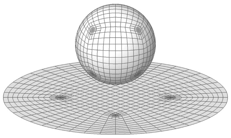
The Bézier elements of the T-spline sphere–plate model. (The sphere is a hollow shell structure.)
The midsurfaces of these shells can be represented exactly using bivariate cubic T-splines [39], allowing an isogeometric discretization. Three T-spline meshes, denoted as M0, M1 and M2, are used in this study. M1 is a global h-refinement of M0, and M2 is an h-refinement of M1. M0, M1 and M2 contain a total of 690, 1565 and 5180 Bézier elements, respectively. The Bézier elements of M1 is shown in Figure 4. The T-spline meshes are generated by the Autodesk T-Splines Plug-in [40] for Rhinoceros [41]. Problems are considered to have reached a static equilibrium configuration when the ℓ∞ norm of the vector of changes in x3-direction displacement unknowns between two time steps is smaller than 10−8. A representative numerical solution is shown in Figure 5. Figure 6a shows the vertical slice cutting through the center of the model, qualitatively demonstrating convergence of the displacement fields.
Figure 5.
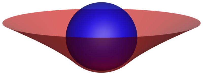
The steady state of the sphere–plate interaction subject to gravitational force.
Figure 6.

Results of mesh independence study of the sphere–plate interaction subject to gravitational force.
To show that quantities of interest associated with contact will converge with mesh refinement, we look at the convergence of the area of the contact region. In our target application of heart valve analysis, area of the contact region, or, the coaptation area (CA), is an important quantitative measure of how effective a valve is at blocking flow [9]. We calculate the CA by integrating the surface area over all Gauss points with nonzero contact forces.5 Figure 6b shows CA as a function of the number of Bézier elements in the model. The relative error in CA satisfies the convergence criterion |CA1 − CA2| < 0.01CA2, where CAi is the CA on mesh Mi.
4.4.2. Sphere–plate impact
It is clear that a spatial semi-discretization of the problem (18) will conserve energy exactly (assuming that B and F derive from potentials, e.g., B from hyperelasticity and F from gravity). To demonstrate that this property can be recovered to a high degree of accuracy in fully discrete solutions, we use a benchmark proposed by Cirak and West [42] and later studied by Vouga et al. [43]. To study energy conservation, we integrate in time with the implicit midpoint rule, which is symplectic [44, Theorem VI.3.5], and can be obtained as a special case of generalized-α integration, with ρ∞ = 1 (i.e., no high-frequency dissipation).
The problem specification is reproduced from [42]. The problem uses the same T-spline mesh M1 as shown in Figure 4, but the sphere and the plate are both free to move. The sphere and the plate initially travel toward one another with a relative velocity of 100. Both objects are modeled as Kirchhoff–Love thin shells of thickness hth = 0.0035. The initial mass density of the shell structures is ρ0 = 0.0785. The constitutive parameters of the sphere and plate are E = 2.1 × 10⁵ and ν = 0.3, as in Section 4.4.1. The parameters used to define the contact potential are p = 4, kc = 10.0, rin/(rout − rmin) = 0.7, rmin/rout = 0.5, and rout = 0.003.
The maximum time step size is set to Δtmax = 10−6. Adaptive time stepping is never triggered for this problem using that time step, even for very small nonlinear convergence tolerances, so Δt = Δtmax in all steps. Several snapshots of the displacement solution are rendered in Figure 7. The kinetic, elastic, contact, and total energies are plotted as functions of time in Figure 8. It is clear that total energy is conserved well. The small proportion of total energy stored as contact potential energy is consistent with the contact potential approximating a workless constraint.
Figure 7.

Snapshots of the sphere–plate impact problem at several time frames.
Figure 8.
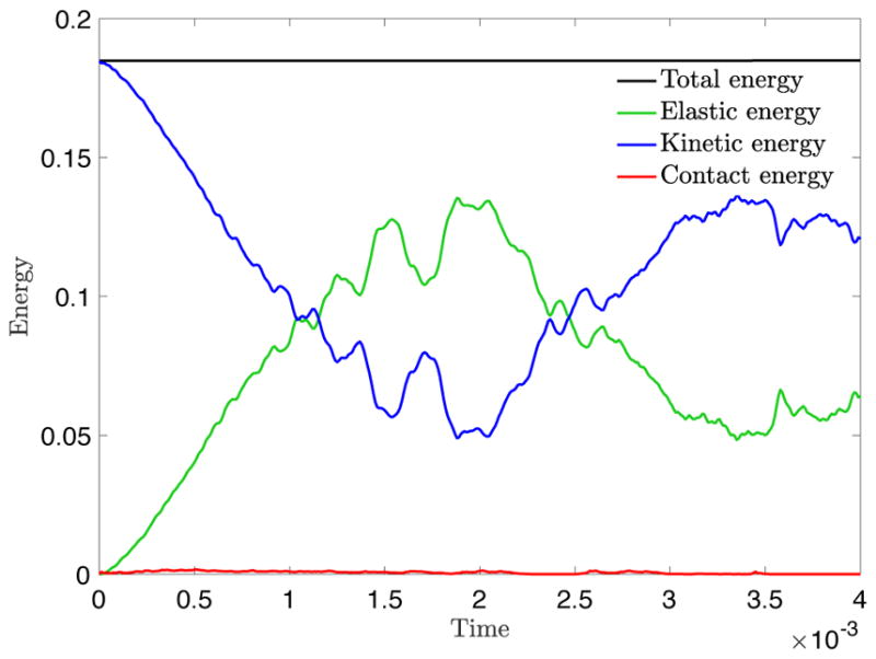
The history of the kinetic, elastic, contact, and total energies for the sphere–plate impact problem.
Remark 5
This benchmark is quite mild from the perspective of nonlinear solution, and the problem can be converged with even larger time steps. However, using too large a time step results in significant energy errors. Energy errors can be induced at the current time step by shrinking the contact length scale rout or increasing the penalty scaling parameter kc (but conservation is still, of course, recovered under refinement in time). Even when using a symplectic integrator, one must use sufficient resolution in time to obtain the oft-cited long-time (near) energy conservation of such methods.6 A way to consistently achieve conservation without tuning of the time step or parameters might be to introduce an additional accuracy-based criterion for time step adaptation, as discussed in Section 3.4, but we have not investigated that possibility thoroughly.
4.4.3. Reef knot
To demonstrate the ability of the proposed approach to handle two-sided self-contact of thin structures with free edges, we introduce a benchmark inspired by the similar reef knot example of [43, Section 8.4]. Two thin 58 cm × 2 cm rectangular ribbons, which consist of 1980 cubic B-spline elements, are positioned as a loosened reef knot. We constrain the ends of the ribbons to move only in the x-direction. To tighten the knot, we prescribe tractions of hnet = ±(104 dyn/cm2)e1 on the regions colored gray in Figure 9. The area of each gray region is 3.2395 cm2, yielding a force (F) with magnitude of 3.2395 × 10⁴ dyn acting on each end of the ribbon. The Young’s modulus of the ribbons is E = 1 × 10⁸ dyn/cm2, the Poisson’s ratio is ν = 0.4, the thickness is 0.004 cm, and the mass density is 1 g/cm3. The parameters defining the contact potential are p = 4, kc = 1.0 × 10⁷ cmp−5s−2g, rin/(rout − rmin) = 0.7, rmin/rout = 0.7, and rout = 0.1 cm. A damping traction of −(10 cm−2s−1g) ẏ is applied to the shell structure midsurface throughout the analysis.
Figure 9.

The reef knot problem setup. Black lines indicate the Bézier elements of the reef knot B-spline surface. This is the stress-free configuration of the ribbons.
Figure 10 shows two snapshot of the reef knot tying simulation at t = 0.08 s and t = 0.4 s. Intersections of the ribbon midsurfaces with a planar slice illustrate the two-sided self-contact of thin structures with free edges. Adaptive time step size over the history of the simulation is shown in Figure 11. It clearly shows that the adaptive subdivision of time step size is triggered when the contact comes into effect. More nonlinear iterations are needed to address the nonlinearity introduced by the numerical contact. As the simulation approaches steady state, the time step size are coarsen until the Δtmax is recovered.
Figure 10.

Results with cross-sectional slices.
Figure 11.
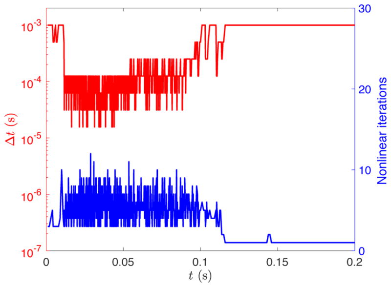
Time step size and number of nonlinear iterations at each time step of the knot-tying simulation.
5. Application to isogeometric analysis of atrioventricular valve dynamics
We now demonstrate the proposed contact methodology, and its integration with isogeometric shell and cable formulations, in the context of a specific application: the structural dynamics of the right atrioventricular valve, also referred to as the tricuspid valve. To focus on issues related to contact, we consider a pure structural mechanics problem, in which the surrounding blood flow is modeled by a pressure load on the valve leaflets and mass-proportional damping.
5.1. Geometrical modeling
We construct an idealized tricuspid valve geometry based on a combination of the model shown in [45] and segmented micro-CT images of porcine tricuspid valves from C.-H. Lee’s lab. The leaflets and chordae are described geometrically by cubic B-spline surfaces and curves. A number of studies have previously found such spline surfaces and curves to be convenient representations of atrioventricular leaflet and chordae geometries extracted from imaging data [14, 46, 47]. The Bézier element meshes of these spline structures are shown in Figure 12. The cross-sectional area of the chordae is about 0.00171 cm2 [45, 48], yielding a chordae radius of 0.023 cm. The leaflet thickness is 0.0396 cm [45, Table 1].
Figure 12.
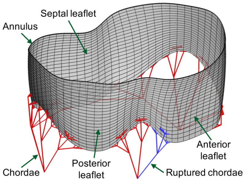
The B-spline surface and elements of the tricuspid valve leaflet and the B-spline chordae.
To demonstrate the capability of the proposed contact methods, we also consider a modification of the geometry described above. We model the atrioventricular valve pathology of prolapse, by severing the chordae highlighted in blue in Figure 12. This pathology is common in the left atrioventricular valve [49], but may also occur in the right side of the heart [50]. Prolapse of atrioventricular valves tends to cause regurgitation (i.e., flow of blood back into the atrium) during systole [1].
5.2. Material modeling
Accurate modeling of tricuspid valve structural mechanics requires careful attention to the constitutive modeling of the leaflet tissue. The extreme nonlinearity of a realistic soft tissue model also serves to test the robustness of the solution algorithm developed in Section 3.4.
5.2.1. Leaflets
To model the leaflet tissue, we assume that the material is incompressible and the second Piola– Kirchhoff stress, S, is computed from the Green–Lagrange strain, E, using an isotropic Fung-type material model, in which the extracellular matrix and fiber stiffness contributions are modeled by neo-Hookean and exponential terms, respectively. Specifically,
| (50) |
where
| (51) |
and
| (52) |
In the above, C = 2E + I is the right Cauchy–Green tensor, p is a Lagrange multiplier enforcing incompressibility7, and c0, c1, and c2 are material parameters. For the tricuspid valve, we use c0 = 10 kPa, c1 = 0.209 kPa, and c2 = 9.046. (c1 and c2 are obtained from [45, Table 2].) The leaflet mass density is 1 g/cm3.
Remark 6
The exponential term in (51) leads to nonlinearities that are especially difficult to resolve. We improve the robustness of our nonlinear solution procedure by assembling the tangent operator (cf. Section 3.4) with a larger value of c0. This requires more iterations, but does not change the converged solution and makes the iterative procedure more robust. In the simulation of valve dynamics, we increase the c0 of the tangent operator to 200 kPa.
Remark 7
Native valve tissue is typically anisotropic, due to collagen fibers being oriented in a preferred direction. Material anisotropy is easily handled by Kirchhoff–Love shell formulations [51–53], but obtaining collagen fiber orientation data, incorporating it into an adequate constitutive model, and calibrating the parameters of that model are challenging research topics outside the scope of the present work, which is primarily focused on contact mechanics.
5.2.2. Chordae
As mentioned in Section 4.2, we restrict the cable material to a simple St. Venant–Kirchhoff model. The St. Venant–Kirchhoff model is typically a poor choice for the stress–strain relation of biological soft tissue about its true reference configuration. However, it can be justified in the case of modeling the tensile response of chordae tendineae, if the reference configuration of the cable is understood to have already been stretched through the chordae’s soft “pre-transition” regime, in which most of the collagen fibers remain slackened and contribute no tensile stiffness. The Young’s modulus of the cable model is then selected to approximate the stiffer “post-transition” regime, in which most of the collagen fibers are recruited. Pre- and post-transition stiffness values for porcine mitral chordae were calculated by fitting ex vivo experimental data in [54, Table 1]. The cited work found that the pre-transition stiffness is several orders of magnitude smaller than the post-transition stiffness. Based on this data, we follow [55] and [56] in neglecting pre-transition stiffness and considering the stress-free reference configuration of the chordae to include tensile strain up to the transition point. For our model of the tricuspid valve, we select a moderately higher effective post-transition stiffness of Eca = 4 × 10⁸ dyn/cm2, in recognition of the fact that tricuspid chordae are typically stiffer [48] than the mitral chordae considered in the cited studies.
5.3. Boundary conditions
Contact in the atrioventricular valves is primarily a concern during systole, when these valves are closed. We simulate valve closure by applying a pressure follower load to the ventricular side of the leaflets. The pressure load as a function of time is
| (53) |
where the ramp-up time scale T is set to T = 0.01 s. The magnitude after time T is representative of normal tricsupid valve pressure gradients during systole [57]. Loss of energy to the surrounding blood is modeled with mass damping, in both the leaflets and the chordae. The damping coefficients Csh and Cca are both 2000 (dyn/g)/(cm/s). The shell structure subproblem is subject to a pinned boundary condition at the annulus. The connections of the chordae to the papillary muscles are subject to strongly-enforced homogeneous Dirichlet boundary conditions on displacement.
5.4. Computational setup
The B-spline surface and curves defining the leaflet and chordal geometry are directly used as an isogeometric computational model. The leaflets consist of 1540 cubic B-spline elements and the chordae contain 373 cubic B-spline elements. The pinned boundary condition at the valve annulus is enforced strongly in the discrete model by fixing the first row of control points. Adaptive time stepping is used with a maximum time step size of Δtmax = 10−4 s. The parameters defining the contact potential are p = 4, kc = 1.0 × 10⁶ g cmp−5 s−2, rin/(rout − rmin) = 0.7, rmin/rout = 0.2, and rout = 0.05 cm.
5.5. Results
The closing behavior of the model with intact chordae is illustrated through a series of snapshots in Figure 13. The complex folding of the valve leaflets is clearly outside the scope of geometries like [4, Figure 20] for which our earlier contact approach was designed, but the potential-based method remains effective. While the closed configuration exhibits creases separating three general “leaflets” (to which the tricuspid valve owes its name), the divisions between these parts of the shell structure are not clear-cut, and self-contact is essential. Figure 14 visualizes the pinballs (Gauss points) on the chordae that are involved in contact. The shell–cable contact and the cable– cable contact are clearly shown. The steady-state configuration shown in Figure 13f is compared, in Figures 15 and 16, with the steady-state configuration resulting from removal of chordae tethering the anterior leaflet. The valve with ruptured chordae clearly exhibits prolapse of the anterior leaflet. The large, visible gap between the leaflets in the prolapsed case clearly illustrates that this pathological condition is associated with regurgitation.
Figure 13.

A series of snapshots illustrating the closing behavior of the tricuspid valve with intact chordae. Color indicates maximum in-plane eigenvalues of E (MIPE) on the atrial side of the leaflets.
Figure 14.
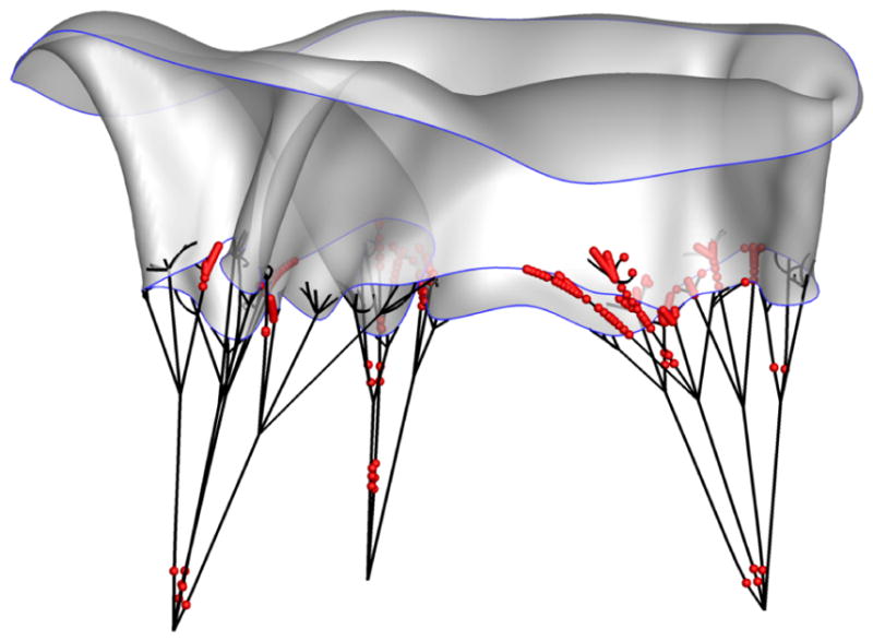
Cable pinballs with nonzero contact forces are highlighted in red, illustrating shell–cable and cable–cable contact. (Recall that pinballs near one another in the reference configuration do not interact.)
Figure 15.

Comparison of coaptation in normal and prolapsing valves.
Figure 16.

Comparison of MIPE contours in normal and prolapsing valves.
Remark 8
The sharp curvature near the free edge of the prolapsed anterior leaflet (visible in Figures 15 and 16) is likely an artifact of our use of a pressure follower load on the ventricular side of the leaflet. This potentially-unphysical solution feature highlights the importance of incorporating fluid–structure interaction into atrioventricular valve prolapse models, as we plan to do in future studies.
6. Conclusion
The contact procedures that we developed in [4, Section 5.2] for isogeometric and immerso-geometric analysis of aortic valves are not suitable for analysis of the more complicated atrioventricular valves. To develop a more versatile formulation, we build on the ideas outlined in [15] and find that, for a particular choice of quadrature and a potential function of limited range, one obtains a discrete scheme with some similarities to the pinball algorithm [20]. Singularities in our new formulation require specialized nonlinear solution and time stepping procedures for reliable convergence. The main limitation of the present study is the need for an ad hoc selection of parameters defining both the contact potential and the solution algorithm. In future extensions, we plan to develop a more principled procedure for selecting parameters. This will reduce computational cost, by avoiding unnecessary refinement in time and/or damping of the nonlinear iteration.
This will enable future immersogeometric fluid–structure interaction (FSI) simulations of atrioventricular valves using the technologies described in this paper for the structural subproblem. As mentioned in Remark 2, we consider the contact methodology discussed in this paper especially well suited for use in conjunction with immersed numerical approaches. However, additional research is required to determine how best to combine the nonlinear solution and adaptive time stepping algorithms described in Section 3.4 with existing FSI solution procedures.
The versatile formulation developed in this paper could also be applied to other challenging problems. The demonstrated effectiveness of our formulation for shell-against-shell contact looks promising in the context of studying damage resulting from impacts against thin composite structures, which some of us have recently become interested in [58]. The formulation’s compatibility with point cloud geometry descriptions also leads us to consider applying it to meshfree discretizations of structures fragmenting after blast loading [59, 60], but the use of an unbounded potential function in explicit computations may lead to difficulties, warranting modifications to the present framework, such as reverting to a non-singular force–separation law.
Acknowledgments
D. Kamensky and Y. Bazilevs were supported through AFOSR Award No. FA9550-16-1-0131. F. Xu and M.-C. Hsu were supported by NIH/NHLBI Award No. R01HL129077. C.-H. Lee was supported by the start-up funds from the AME School at the University of Oklahoma (OU) and the American Heart Association Scientist Development Grant Award (16SDG27760143). The micro-CT scanning service provided by Dr. Hong Liu at the OU Advanced Medical Imaging Core Facility is greatly acknowledged. The assistance from Katie Kramer for image segmentation of the tricuspid valve geometry is greatly appreciated.
Footnotes
Another interesting approach to avoiding nonlocal interactions is to store contact potential energy as elastic potential energy of a fictitious material filling the void between objects [18, 19].
Asymptotic notation in this section follows standard computer science conventions. See, e.g., [27].
Note that, in the present document, this is distinguished from “big 𝒪” asymptotic notation by font.
This structure is inspired by the cluster maps used in FAT file systems.
Tacit in this definition of CA is the assumption that rout is small relative to the overall length scale of the structure geometry. If rout were large relative to the structure, the entire surface of the structure would carry contact forces, and convergence of CA would be trivial.
It is possible to conserve energy exactly [44, Section IV.4], but this can actually disrupt the good qualitative behavior of symplectic integration that is frequently (and perhaps misleadingly) attributed to good long-time energy conservation [44, Example IV.4.4].
For shell analysis, one can use the plane stress condition, S33 = 0, to analytically determine the Lagrangian multiplier p (see Kiendl et al. [34, Section 5.1] for details).
Publisher's Disclaimer: This is a PDF file of an unedited manuscript that has been accepted for publication. As a service to our customers we are providing this early version of the manuscript. The manuscript will undergo copyediting, typesetting, and review of the resulting proof before it is published in its final citable form. Please note that during the production process errors may be discovered which could affect the content, and all legal disclaimers that apply to the journal pertain.
References
- 1.Hayek E, Gring CN, Griffin BP. Mitral valve prolapse. The Lancet. 2005;365(9458):507–518. doi: 10.1016/S0140-6736(05)17869-6. [DOI] [PubMed] [Google Scholar]
- 2.Chandran KB. Role of computational simulations in heart valve dynamics and design of valvular prostheses. Cardiovascular Engineering and Technology. 2010;1(1):18–38. doi: 10.1007/s13239-010-0002-x. [DOI] [PMC free article] [PubMed] [Google Scholar]
- 3.Kheradvar A, Groves EM, Falahatpisheh A, Mofrad MK, Hamed Alavi S, Tranquillo R, Dasi LP, Simmons CA, Grande-Allen KJ, Goergen CJ, Baaijens F, Little SH, Canic S, Griffith B. Emerging trends in heart valve engineering: Part IV. Computational modeling and experimental studies. Annals of Biomedical Engineering. 2015;43(10):2314–2333. doi: 10.1007/s10439-015-1394-4. [DOI] [PubMed] [Google Scholar]
- 4.Kamensky D, Hsu M-C, Schillinger D, Evans JA, Aggarwal A, Bazilevs Y, Sacks MS, Hughes TJR. An immersogeometric variational framework for fluid–structure interaction: Application to bioprosthetic heart valves. Computer Methods in Applied Mechanics and Engineering. 2015;284:1005–1053. doi: 10.1016/j.cma.2014.10.040. [DOI] [PMC free article] [PubMed] [Google Scholar]
- 5.Hsu M-C, Kamensky D, Bazilevs Y, Sacks MS, Hughes TJR. Fluid–structure interaction analysis of bioprosthetic heart valves: significance of arterial wall deformation. Computational Mechanics. 2014;54:1055–1071. doi: 10.1007/s00466-014-1059-4. [DOI] [PMC free article] [PubMed] [Google Scholar]
- 6.Hsu M-C, Kamensky D, Xu F, Kiendl J, Wang C, Wu MCH, Mineroff J, Reali A, Bazilevs Y, Sacks MS. Dynamic and fluid–structure interaction simulations of bioprosthetic heart valves using parametric design with T-splines and Fung-type material models. Computational Mechanics. 2015;55:1211–1225. doi: 10.1007/s00466-015-1166-x. [DOI] [PMC free article] [PubMed] [Google Scholar]
- 7.Kamensky D, Hsu M-C, Yu Y, Evans JA, Sacks MS, Hughes TJR. Immersogeometric cardiovascular fluid–structure interaction analysis with divergence-conforming B-splines. Computer Methods in Applied Mechanics and Engineering. 2017;314:408–472. doi: 10.1016/j.cma.2016.07.028. [DOI] [PMC free article] [PubMed] [Google Scholar]
- 8.Aggarwal A, Sacks MS. An inverse modeling approach for semilunar heart valve leaflet mechanics: exploitation of tissue structure. Biomechanics and Modeling in Mechanobiology. 2016;15(4):909–932. doi: 10.1007/s10237-015-0732-7. [DOI] [PubMed] [Google Scholar]
- 9.Morganti S, Auricchio F, Benson DJ, Gambarin FI, Hartmann S, Hughes TJR, Reali A. Patient-specific isogeometric structural analysis of aortic valve closure. Computer Methods in Applied Mechanics and Engineering. 2015;284:508–520. [Google Scholar]
- 10. [Accessed 17 July 2016];LS-DYNA Finite Element Software: Livermore Software Technology Corp. http://www.lstc.com/products/ls-dyna.
- 11. [Accessed 6 April 2017];Simulia. http://www.3ds.com/products-services/simulia/
- 12.Lee C-H, Amini R, Gorman RC, Gorman JH, Sacks MS. An inverse modeling approach for stress estimation in mitral valve anterior leaflet valvuloplasty for in-vivo valvular biomaterial assessment. J Biomech. 2014;47(9):2055–2063. doi: 10.1016/j.jbiomech.2013.10.058. [DOI] [PMC free article] [PubMed] [Google Scholar]
- 13.Lee C-H, Amini R, Sakamoto Y, Carruthers CA, Aggarwal A, Gorman RC, Gorman JH, Sacks MS. Mitral valves: A computational framework. In: De S, Hwang W, Kuhl E, editors. Multiscale Modeling in Biomechanics and Mechanobiology. Springer; London: 2015. pp. 223–255. [Google Scholar]
- 14.Lee C-H, Rabbah JP, Yoganathan AP, Gorman RC, Gorman JH, Sacks MS. On the effects of leaflet microstructure and constitutive model on the closing behavior of the mitral valve. Biomechanics and Modeling in Mechanobiology. 2015;14(6):1281–1302. doi: 10.1007/s10237-015-0674-0. [DOI] [PMC free article] [PubMed] [Google Scholar]
- 15.Sauer RA, De Lorenzis L. A computational contact formulation based on surface potentials. Computer Methods in Applied Mechanics and Engineering. 2013;253(0):369–395. [Google Scholar]
- 16.Barnes J, Hut P. A hierarchical O(N log N) force-calculation algorithm. Nature. 1986;324(6096):446–449. [Google Scholar]
- 17.Rokhlin V. Rapid solution of integral equations of classical potential theory. Journal of Computational Physics. 1985;60(2):187–207. [Google Scholar]
- 18.Wriggers P, Schröder J, Schwarz A. A finite element method for contact using a third medium. Computational Mechanics. 2013;52(4):837–847. [Google Scholar]
- 19.Bog T, Zander N, Kollmannsberger S, Rank E. Normal contact with high order finite elements and a fictitious contact material. Computers & Mathematics with Applications. 2015;70(7):1370–1390. [Google Scholar]
- 20.Belytschko T, Neal MO. Contact-impact by the pinball algorithm with penalty and Lagrangian methods. International Journal for Numerical Methods in Engineering. 1991;31(3): 547–572. [Google Scholar]
- 21.Sauer RA. PhD thesis. University of California, Berkeley; Berkeley, California: 2006. An Atomic Interaction based Continuum Model for Computational Multiscale Contact Mechanics. [Google Scholar]
- 22.Guan PC, Chi SW, Chen JS, Slawson TR, Roth MJ. Semi-Lagrangian reproducing kernel particle method for fragment-impact problems. International Journal of Impact Engineering. 2011;38(12):1033–1047. [Google Scholar]
- 23.Peskin CS. Flow patterns around heart valves: A numerical method. Journal of Computational Physics. 1972;10(2):252–271. [Google Scholar]
- 24.Sulsky D, Chen Z, Schreyer HL. A particle method for history-dependent materials. Computer Methods in Applied Mechanics and Engineering. 1994;118(1):179–196. [Google Scholar]
- 25.Baaijens FPT. A fictitious domain/mortar element method for fluid–structure interaction. International Journal for Numerical Methods in Fluids. 2001;35(7):743–761. [Google Scholar]
- 26.Kadapa C, Dettmer WG, Perić D. A stabilised immersed boundary method on hierarchical b-spline grids for fluid–rigid body interaction with solid–solid contact. Computer Methods in Applied Mechanics and Engineering. 2017;318:242–269. [Google Scholar]
- 27.Cormen TH, Stein C, Rivest RL, Leiserson CE. Introduction to Algorithms. 2. McGraw-Hill Higher Education; 2001. [Google Scholar]
- 28.Belytschko T, Yeh IS. The splitting pinball method for general contact. Proceedings of the 10th International Conference on Computing Methods in Applied Sciences and Engineering on Computing Methods in Applied Sciences and Engineering; Commack, NY, USA. Nova Science Publishers, Inc; 1991. pp. 73–87. [Google Scholar]
- 29.Belytschko T, Yeh IS. The splitting pinball method for contact-impact problems. Computer Methods in Applied Mechanics and Engineering. 1993;105(3):375–393. [Google Scholar]
- 30.Casadei F, Aune V, Valsamos G, Larcher M. Technical Report JRC101013. European Commission: Joint Research Centre; 2016. Generalization of the pinball contact/ impact model for use with mesh adaptivity and element erosion in EUROPLEXUS. [Google Scholar]
- 31.Livermore Software Technology Corporation. LS-DYNA keyword user’s manual R8.0. 2015;I [Google Scholar]
- 32.Bazilevs Y, Calo VM, Hughes TJR, Zhang Y. Isogeometric fluid–structure interaction: theory, algorithms, and computations. Computational Mechanics. 2008;43:3–37. [Google Scholar]
- 33.Gomez H, Hughes TJR. Provably unconditionally stable, second-order time-accurate, mixed variational methods for phase-field models. Journal of Computational Physics. 2011;230(13):5310–5327. [Google Scholar]
- 34.Kiendl J, Hsu M-C, Wu MCH, Reali A. Isogeometric Kirchhoff–Love shell formulations for general hyperelastic materials. Computer Methods in Applied Mechanics and Engineering. 2015;291:280–303. doi: 10.1016/j.cma.2015.05.006. [DOI] [PMC free article] [PubMed] [Google Scholar]
- 35.Temizer İ, Wriggers P, Hughes TJR. Contact treatment in isogeometric analysis with NURBS. Computer Methods in Applied Mechanics and Engineering. 2011;200(9):1100–1112. [Google Scholar]
- 36.Temizer İ, Wriggers P, Hughes TJR. Three-dimensional mortar-based frictional contact treatment in isogeometric analysis with NURBS. Computer Methods in Applied Mechanics and Engineering. 2012;209:115–128. [Google Scholar]
- 37.De Lorenzis L, Temizer İ, Wriggers P, Zavarise G. A large deformation frictional contact formulation using NURBS-based isogeometric analysis. International Journal for Numerical Methods in Engineering. 2011;87(13):1278–1300. [Google Scholar]
- 38.Raknes SB, Deng X, Bazilevs Y, Benson DJ, Mathisen KM, Kvamsdal T. Isogeometric rotation-free bending-stabilized cables: Statics, dynamics, bending strips and coupling with shells. Computer Methods in Applied Mechanics and Engineering. 2013;263:127–143. [Google Scholar]
- 39.Sederberg TW, Cardon DL, Finnigan GT, North NS, Zheng J, Lyche T. T-spline simplification and local refinement. ACM Transactions on Graphics. 2004;23(3):276–283. [Google Scholar]
- 40.Autodesk T-Splines Plug-in for Rhino. 2015 http://www.tsplines.com/products/tsplines-for-rhino.html.
- 41.Rhinoceros. [Accessed 19 July 2016]; http://www.rhino3d.com/
- 42.Cirak F, West M. Decomposition contact response (DCR) for explicit finite element dynamics. International Journal for Numerical Methods in Engineering. 2005;64(8):1078–1110. [Google Scholar]
- 43.Vouga E, Harmon D, Tamstorf R, Grinspun E. Asynchronous variational contact mechanics. Computer Methods in Applied Mechanics and Engineering. 2011;200(2528):2181– 2194. [Google Scholar]
- 44.Hairer E, Wanner G, Lubich C. Geometric Numerical Integration: Structure-Preserving Algorithms for Ordinary Differential Equations. Springer Berlin Heidelberg; Berlin, Heidelberg: 2006. [Google Scholar]
- 45.Stevanella M, Votta E, Lemma M, Antona C, Redaelli A. Finite element modelling of the tricuspid valve: A preliminary study. Medical Engineering & Physics. 2010;32(10):1213–1223. doi: 10.1016/j.medengphy.2010.08.013. [DOI] [PubMed] [Google Scholar]
- 46.Drach A, Khalighi AH, ter Huurne FM, Lee C-H, Bloodworth C, Pierce EL, Jensen MO, Yoganathan AP, Sacks MS. Population-averaged geometric model of mitral valve from patient-specific imaging data. Journal of Medical Devices. 2015;9(3):030952-1–030952-3. [Google Scholar]
- 47.Khalighi AH, Drach A, Bloodworth CH, Pierce EL, Yoganathan AP, Gorman RC, Gorman JH, Sacks MS. Mitral valve chordae tendineae: Topological and geometrical characterization. Annals of Biomedical Engineering. 2017;45(2):378–393. doi: 10.1007/s10439-016-1775-3. [DOI] [PMC free article] [PubMed] [Google Scholar]
- 48.Lim KO. Mechanical properties and ultrastructure of normal human tricuspid valve chordae tendineae. The Japanese Journal of Physiology. 1980;30(3):455–464. doi: 10.2170/jjphysiol.30.455. [DOI] [PubMed] [Google Scholar]
- 49.Freed LA, Levy D, Levine RA, Larson MG, Evans JC, Fuller DL, Lehman B, Benjamin EJ. Prevalence and clinical outcome of mitral-valve prolapse. New England Journal of Medicine. 1999;341(1):1–7. doi: 10.1056/NEJM199907013410101. [DOI] [PubMed] [Google Scholar]
- 50.Raichlen JS, Brest AN. Tricuspid valve prolapse. Cardiovascular Clinics. 1987;17(2): 97–109. [PubMed] [Google Scholar]
- 51.Buganza Tepole A, Kabaria H, Bletzinger K-U, Kuhl E. Isogeometric kirchhoff–love shell formulations for biological membranes. Computer Methods in Applied Mechanics and Engineering. 2015;293:328–347. doi: 10.1016/j.cma.2015.05.006. [DOI] [PMC free article] [PubMed] [Google Scholar]
- 52.Roohbakhshan F, Sauer RA. Efficient isogeometric thin shell formulations for soft biological materials. Biomechanics and Modeling in Mechanobiology. 2017;16(5):1569–1597. doi: 10.1007/s10237-017-0906-6. [DOI] [PubMed] [Google Scholar]
- 53.Wu MCH, Zakerzadeh R, Kamensky D, Kiendl J, Sacks MS, Hsu M-C. An anisotropic constitutive model for immersogeometric fluid–structure interaction analysis of bioprosthetic heart valves. Journal of Biomechanics. 2017 doi: 10.1016/j.jbiomech.2018.04.012. In review. [DOI] [PMC free article] [PubMed] [Google Scholar]
- 54.Kunzelman KS, Cochran RP. Stress/strain characteristics of porcine mitral valve tissue: parallel versus perpendicular collagen orientation. Journal of Cardiac Surgery. 1992;7(1): 71–78. doi: 10.1111/j.1540-8191.1992.tb00777.x. [DOI] [PubMed] [Google Scholar]
- 55.Krishnamurthy G, Ennis DB, Itoh A, Bothe W, Swanson JC, Karlsson M, Kuhl E, Miller DC, Ingels NB. Material properties of the ovine mitral valve anterior leaflet in vivo from inverse finite element analysis. American Journal of Physiology–Heart and Circulatory Physiology. 2008;295(3):H1141–H1149. doi: 10.1152/ajpheart.00284.2008. [DOI] [PMC free article] [PubMed] [Google Scholar]
- 56.Rausch MK, Famaey N, Shultz TO, Bothe W, Miller DC, Kuhl E. Mechanics of the mitral valve: a critical review, an in vivo parameter identification, and the effect of prestrain. Biomechanics and Modeling in Mechanobiology. 2013;12(5):1053–1071. doi: 10.1007/s10237-012-0462-z. [DOI] [PMC free article] [PubMed] [Google Scholar]
- 57.Aessopos A, Farmakis D, Taktikou H, Loukopoulos D. Doppler-determined peak systolic tricuspid pressure gradient in persons with normal pulmonary function and tricuspid regurgitation. Journal of the American Society of Echocardiography. 2000;13(7):645–649. doi: 10.1067/mje.2000.104535. [DOI] [PubMed] [Google Scholar]
- 58.Pigazzini M, Bazilevs Y, Benson D, Kim H, Ellison A. Isogeometric analysis of damage and residual-strength in aerospace composite structures subjected to low-velocity impact. Proceedings of the American Society for Composites: Thirty-First Technical Conference; 2016. [Google Scholar]
- 59.Bazilevs Y, Kamran K, Moutsanidis G, Benson DJ, Oñate E. A new formulation for air-blast fluid–structure interaction using an immersed approach. Part I: basic methodology and FEM-based simulations. Computational Mechanics. 2017;60(1):83–100. [Google Scholar]
- 60.Bazilevs Y, Moutsanidis G, Bueno J, Kamran K, Kamensky D, Hillman MC, Gomez H, Chen JS. A new formulation for air-blast fluid–structure interaction using an immersed approach: Part II—coupling of IGA and meshfree discretizations. Computational Mechanics. 2017;60(1):101–116. [Google Scholar]