Realistic modeling of deep brain stimulation implants for electromagnetic MRI safety studies

Abstract

We propose a framework for electromagnetic (EM) simulation of deep brain stimulation (DBS) patients in radiofrequency (RF) coils. We generated a model of a DBS patient using post-operative head and neck computed tomography (CT) images stitched together into a “virtual CT” image covering the entire length of the implant. The body was modeled as homogeneous. The implant path extracted from the CT data contained self-intersections, which we corrected automatically using an optimization procedure. Using the CT-derived DBS path, we built a model of the implant including electrodes, helicoidal internal conductor wires, loops, extension cables, and the implanted pulse generator. We also built four simplified models with straight wires, no extension cables and no loops to assess the impact of these simplifications on safety predictions. We simulated EM fields induced by the RF birdcage body coil in the body model, including at the DBS lead tip at both 1.5 Tesla (64 MHz) and 3 Tesla (123 MHz). We also assessed the robustness of our simulation results by systematically varying the EM properties of the body model and the position and length of the DBS implant (sensitivity analysis). The topology correction algorithm corrected all self-intersection and curvature violations of the initial path while introducing minimal deformations (open-source code available at http://ptx.martinos.org/index.php/Main_Page). The unaveraged lead-tip peak SAR predicted by the five DBS models (0.1 mm resolution grid) ranged from 12.8 kW/kg (full model, helicoidal conductors) to 43.6 kW/kg (no loops, straight conductors)at 1.5 T (3.4-fold variation) and 18.6 kW/kg (full model, straight conductors) to 73.8 kW/kg (no loops, straight conductors)at 3 T (4.0-fold variation). At 1.5 T and 3 T, the variability of lead-tip peak SAR with respect to the conductivity ranged between 18% and 30%. Variability with respect to the position and length of the DBS implant ranged between 9.5% and 27.6%.

Introduction

Deep brain stimulation (DBS) is a neuromodulation approach used to treat severe Parkinson disease and other movement disorders (Deuschl et al., 2006; Weaver et al., 2009; Vidailhet et al., 2005). Although the clinical benefits of DBS are well established for movement disorders, its mechanisms of action are not well understood (McIntyre et al., 2004; Widge et al., 2015; Widge and Dougherty, 2015; Herrington et al., 2016). DBS has been suggested as a possible therapy for intractable psychiatric disorders such as treatment-resistant depression (TRD) (Mayberg et al., 2005; Malone Jr et al., 2009; Schlaepfer et al., 2007; Bewernick et al., 2010; Puigdemont et al., 2011) and obsessive-compulsive disorder (Greenberg et al., 2006; Denys et al., 2010; Huff et al., 2010) but the lack of a clear understanding of its mechanisms of action is a major hurdle to large-scale clinical adoption (Widge et al., 2015; Widge and Dougherty, 2015). Of all the clinical imaging modalities, MRI is unique in that it allows mapping both the anatomical (diffusion MRI) and functional (functional MRI, fMRI) brain networks. In addition, MRI has great grey matter-white matter contrast, which can be helpful for localization of the DBS electrodes (anatomical, diffusion and functional scans can be obtained in a single session).

Despite these strengths, MRI is often counter-indicated in DBS patients because of the risk of thermal injury (Henderson et al., 2005). This is due to electromagnetic (EM) coupling between the MRI radiofrequency (RF) coil and the DBS metallic leads (Yeung and Atalar, 2001; Finelli et al., 2002; Park et al., 2005; Park et al., 2007; Angelone et al., 2008; Neufeld et al., 2009; Bottomley et al., 2010; Acikel and Atalar, 2011; Eryaman et al., 2011; Bonmassar et al., 2013; Iacono et al., 2013; Acikel et al., 2016; Golestanirad et al., 2016a). As a result, MRI is seldom used in DBS patients. Until recently, the guidelines for safe MR imaging of patients implanted with Medtronic DBS systems required using a 1.5 T scanner and a global SAR (=average SAR) smaller than 0.1 W/kg (Medtronics, 2015), which is 30x smaller than the IEC recommended power limit for patients with no implants (Commission, 2010). The most recent version of these guidelines prescribes a maximum root mean square B1+ (the right-handed circularly polarized component of the magnetic field projected onto the transverse plane) value of 2 μT for the whole scan – it is not clear yet how this limit compares with the former global SAR limit. For high-SAR clinical sequences such as fluid attenuated inversion recovery (De Coene et al., 1992) and turbo spin echo (Hennig et al., 1986), this low-power requirement may negatively impact image quality. From a research standpoint, the Medtronic guidelines restriction to 1.5 T scanning is a significant constraint, because the study of the neural networks affected by the DBS treatment using functional MRI would be best performed at higher field strengths such as 3 T or 7 T. Indeed, the signal-to-noise ratio (SNR) and BOLD contrast (ΔR2*/R2*) are both 2x greater at 3 T than at 1.5 T, resulting in a 4-fold increase of the contrast-to-noise ratio (CNR) of fMRI studies. At 7 T, the BOLD CNR is 22x greater than at 1.5 T. These dramatic gains in fMRI precision and sensitivity at ultra-high fields have been used to study the fine-scale structure (<1 mm) of cortical layer activations in patients without implants (Polimeni et al., 2010). Similar high-resolution fMRI studies in DBS patients could reveal detailed maps of the functional networks modulated by the DBS treatment -- in contrast, current fMRI studies of DBS patients at 1.5 T are typically limited to ~4 mm linear resolution (Figee et al., 2013).

EM simulations are useful to study the RF interactions between the DBS implant and the MRI coil. Despite the relatively large body of literature on this topic, to our knowledge most previously published studies have simulated highly simplified DBS implant models. For example, the geometrical path modeled often does not include lead loops (whereas in reality DBS leads are coiled over the skull) (Park et al., 2005; Neufeld et al., 2009; Angelone et al., 2010; Eryaman et al., 2011; Mohsin, 2011; Eryaman et al., 2012; Bonmassar et al., 2013; Cabot et al., 2013; Iacono et al., 2013; Eryaman et al., 2014; Serano et al., 2014), no extension cable (Mohsin et al., 2008; Neufeld et al., 2009; Angelone et al., 2010; Eryaman et al., 2011; Mohsin, 2011; Eryaman et al., 2012; Iacono et al., 2013; Cabot et al., 2013; Eryaman et al., 2014; Golestanirad et al., 2016b; Golestanirad et al., 2016a) and have straight internal wires instead of the helicoidal wiring used in commercially available systems (Park et al., 2005; Mohsin et al., 2008; Neufeld et al., 2009; Angelone et al., 2010; Mohsin, 2011; Eryaman et al., 2011; Eryaman et al., 2012; Bonmassar et al., 2013; Iacono et al., 2013; Eryaman et al., 2014; Serano et al., 2014; Golestanirad et al., 2016b; Golestanirad et al., 2016a). These simplifications may lead to incorrect estimates of the implant electrical length, and ultimately of the SAR and temperature predictions.

In this work, we develop a patient-specific DBS-MRI EM simulation methodology with accurate modeling of the geometrical path of the DBS implant as well as most of its internal structure. Our methodology allows efficient (<5 hours) generation of DBS models based on patient CT images that include loops, extension cables, and the implanted pulse generator (IPG). A key component of the method is a topology correction algorithm that automatically removes self-intersections and curvature violations in the path estimated from the CT data (code available at http://ptx.martinos.org/index.php/Main_Page). We model the RF interactions between the DBS implant and the MRI coil using a simulation strategy based on the field solver HFSS (Kozlov and Turner, 2009; Guérin et al., 2014; Guérin et al., 2015), which allows efficient modeling of the smallest implant details (simulation time ~6 hours). We find that detailed modeling of the DBS implant path and internal components has a large impact on the SAR induced at the electrode-tissue interface tip by the MRI RF coil. We hope that this simulation methodology can be helpful to other researchers to further study the interaction between the MRI RF coil and the DBS implant. We apply our framework to the simulation of a bilateral DBS patient inside a body birdcage coil operating at 1.5 and 3 Tesla. We evaluate the impact of several simplifications of the DBS lead model on SAR predictions. Although these results cannot be extrapolated into universal trends (this would require simulation of hundreds of patients and MRI coil configurations), they show the importance of accurate modeling of the DBS path and internal components for robust, DBS patient-specific SAR prediction.

Methods

Extraction of the DBS implant path from CT images

We created a model of a 70 year-old male who received DBS of the subthalamic nucleus at Massachusetts General Hospital (PATIENT 1). As per usual clinical procedure, this patient received a high-resolution head computer tomography (CT) scan after the first surgery (implantation of the DBS leads) and an X-ray after the second (implantation of the extension cables and IPG). Years later, the patient received a high-resolution neck CT scan for reasons unrelated to his DBS treatment. The field-of-view (FOV) of the head CT volume extended from the upper jaw to the top of the head, whereas that of the neck CT extended from the upper lungs to the frontal lobe. None of these volumes completely covered the entire length of the implant, therefore we co-registered them manually using FreeView (https://surfer.nmr.mgh.harvard.edu/fswiki/FreeviewGuide) and stitched them together to obtain a composite, full DBS-length CT volume (Fig. 1, STEP #1). The seamline was located around the mid-head level (red arrows on Fig. 1, STEP #1) since in this area anatomical structures do not move as much as in the jaw region.

Fig 1.

Process for semi-automatic extraction of the DBS lead path from CT data. STEP #1: If a single CT scan is not available that covers the entire path of the DBS implant, we stitch the head and neck CT volumes into a single “virtual CT” volume. STEP #2: The CT voxels corresponding to the DBS leads are segmented by simple thresholding followed by manual cleanup. STEP #3: The “skeleton” of the thresholded DBS path is reconstructed, which is a 1-voxel thick representation of the connected branches forming the DBS path. STEP #4: The branches corresponding to the left (L) and right (R) DBS leads are connected in a continuous path manually. Care must be taken that the loops in the model are coiled in the same way as in the CT volume. STEP #5: The L/R DBS leads are smoothed and resampled. STEP #6: The distances between every pair of segments belonging to the L/R DBS leads are computed. Black thick lines correspond to segment pairs that are closer than the minimal distance, which is the diameter of the DBS external insulation layer. STEP #7: Our automatic topology correction algorithm is run to correct all path intersections and resolve unphysical curvatures.

We segmented the DBS cables by thresholding (Fig. 1, STEP #2). Manual cleanup of the resulting DBS mask was required because the skull and metal screws have Hounsfield units very similar to that of the DBS cables. We then extracted the centerline of the segmented DBS volume using the skeletonization algorithm in FIJI (https://fiji.sc/, Fig. 1, STEP #3). This resulted in a set of disconnected segments, which we connected manually (Fig. 1, STEP #4). Finally, we smoothed the left and right DBS paths to minimize CT voxelization artefacts (staircasing) and resampled them using the Ramer-Douglas-Peucker algorithm (Douglas and Peucker, 1973). This last step was applied to yield path representations with many points in regions of high tortuosity and few points in regions with little variation (Fig. 1, STEP #5).

Automatic topology correction of the DBS path

In this paper, we denote vectors and matrices in bold and scalars in regular type. The path representation obtained after Fig. 1, STEP #5 is a collection of 3D points connected by straight lines. This path representation contained topological defects such as self-intersections (i.e., two segments closer than the cable diameter) and curvature violations (i.e., local curvature smaller than 1/R, where R is the cable diameter). Fig. 1, STEP #6 consists in detecting these defects. We parameterize the linear segments joining points x and y as L(x, y)={(y – x) t + x | t ∈ [0;1]}, where t is the free parameter. Moreover, we define the distance D(L₁, L₂) between the segments L₁ and L₂ as the smallest distance between any two points belonging to these segments. This distance definition is, in general, different from the distance between the two extreme points of the segments (Fig. 4, “a” and “b”). D(·) is computed by solving the following constrained optimization problem:

$$\begin{gathered} D{\left\{L\left({\mathbf{x}}_1,{\mathbf{y}}_1\right),L\left({\mathbf{x}}_2,{\mathbf{y}}_2\right)\right\}}^2=\underset{t_1,t_2}{min}{\Vert \left[\left({\mathbf{y}}_1-{\mathbf{x}}_1\right)t_1+{\mathbf{x}}_1\right]-\left[\left({\mathbf{y}}_2-{\mathbf{x}}_2\right)t_2+{\mathbf{x}}_2\right]\Vert }^2\text{s.t.}0\le t_1,t_2\le 1 \\ =\underset{t_1,t_2}{min}\left\{{\Vert \mathbf{a}\Vert }^2{t}_1^2+{\Vert \mathbf{c}\Vert }^2{t}_2^2-2t_1{t}_2\mathbf{a}·\mathbf{c}+2t_1\mathbf{a}·\mathbf{\Delta }-2t_2\mathbf{c}·\mathbf{\Delta }+{\Vert \mathbf{\Delta }\Vert }^2\right\}\text{s.t.}0\le t_1,t_2\le 1, \end{gathered}$$ [1]

where a = y₁ – x₁, c = y₂ – x₂, Δ = x₁ – x₂ and t₁ and t₂ are the free parameters of linear segments L(x₁, y₁) and L(x₂, y₂), respectively. This problem is easily solved by first solving analytically the unconstrained quadratic minimization problem and then checking the boundary conditions (there are only four cases to check: t₁ = 0, t₁ = 1, t₂ = 0 and t₂ = 1). In order to detect all possible intersections of the path, including those between segments of the left lead and segments of the right lead, we concatenated the left and right DBS lead paths and ran the distance calculation on this composite path.

Fig. 4.

A: Picture of the five 3D-printed DBS tubular models. B: Close-up of one of the 3D-printed model. The central copper wire is inserted in the central groove of the hollow tube. The picture also shows clearly the ladder of vertical filaments supporting the tube. C: Picture of a 3D-printed model in a plastic sphere partially filled with agar gel. After the track was placed on the solidified agar, the sphere was closed and sealed and hot liquid agar gel was poured through a small hole. D: RMSD, minimum and maximum distance between the reconstructed and reference DBS path (all quantities are expressed in mm). The bar graph shows the averaged quantities for the five 3D-printed DBS models and the error bars show the standard deviation. E: Visualization of the five reference (red) and reconstructed paths (blue).

Once we determined the intersecting path locations, we corrected them by solving the following optimization problem (Fig. 1, STEP #7):

$$\begin{gathered} \widehat{\mathbf{X}}=\underset{\mathbf{X}}{argmin}{\Vert \mathbf{X}-{\mathbf{X}}_0\Vert }^2 \\ \text{subject}\text{to:} \\ (\mathrm{a})K_i\le \raisebox{1ex}{$1$}\!\left/ \!\raisebox{-1ex}{$R$}\right.\forall i \\ (\mathrm{b})D\{L({\mathbf{x}}_i,{\mathbf{x}}_{i+1}),L({\mathbf{x}}_i,{\mathbf{x}}_{i+1})\}\ge 2R\forall k\ge i+i_{min}, \end{gathered}$$ [2]

where X̂ and X₀ are the optimized and the initial (derived from the CT data) path representations, respectively (those N×3 matrices, where N is the number of points in the path). The objective function in Eq. [2] forces the corrected path to be as close as possible to the initial path estimate. Constraints (a) impose that the path curvature at every point of the path (K_i) is smaller than the inverse of the DBS cable radius (R), which is a physical constraint. Constraints (b) impose that the distance between any pair of segments is greater than the cable diameter 2R (note that this is imposed for segments number separated by i_min, with i_min > 1 since consecutive segments are touching and therefore have, by definition, D = 0). We solve this optimization problem using the active-set algorithm without derivatives as implemented in Matlab (“fmincon”). This Matlab code is available online at http://ptx.martinos.org/index.php/Main_Page.

Modeling of the DBS internal structure

The non-intersecting left and right DBS paths obtained in Fig. 1, STEP #7 form the skeleton of the DBS implant model (in this work, we modeled the Medtronic lead 3387 which has four 1.5 mm-long electrodes separated by 1.5 mm gaps). We straightened the tip of the left and right DBS leads because Medtronic electrode tips are rigid (Fig. 2, STEP #1). We then segmented the left and right DBS cables into two portions: The lead cable (defined as the first 40 cm of the path, starting from the electrode tip) and the extension cable (remaining 40 cm of the path). This was required since the lead and extension cables have different diameters and their internal conductive wires are laid out differently.

Fig. 2.

Creation of the full DBS implant model from the non-intersecting DBS path. STEP #1: The wireframe DBS model is straightened at the electrode tips since the lead is rigid at this location. STEP #2: Four cable conductors are created around the main DBS path. The four conductor wires are braided in the lead region and run parallel in the extension cable region of the implant. STEP #3: The IPG (green box) is added to the model as well as small line segments connecting the four main conductor paths to the electrodes (top zoom box) and the IPG (bottom zoom box). STEP #4: All the line segments are imported in HFSS and are thickened to their physical diameter. This allows creation of the electrodes, conductor paths and insulation sleeves. The four main conductor paths are connected to the IPG via 2000 Ω resistors modeling the input impedance of the IPG.

The next step was to add the internal wiring (Fig. 2, STEP #2). In Medtronic devices, internal wires have tightly wound helicoidal trajectories that are braided (lead cable) or run in parallel to each other (extension cable). For the lead cable, we generated four co-axial braided helices using the “helix along curve” tool in Sketchup. For the extension cable, we first created four paths separated by 1 mm and running parallel to the main path and then wound helices around these. In this work, we modeled helices with 2 mm pitch for both the lead and extension cables. This is much greater than the pitch of helicoidal wires in the Medtronic lead 3387 (~0.33 mm), however we have found it difficult to model tightly wound helices along arbitrary paths in HFSS (see Discussion section).

The third step (Fig. 2, STEP #3) was to add small linear segments to the conductive wires for connection to the electrodes and the IPG. Finally (Fig. 2, STEP #4), we added the electrodes to the model and created the insulation sleeve for the lead (diameter=1.27 mm) and extension cables (diameter=2.43 mm). Most of the operations described in this section were scripted within Ansys HFSS using Visual Basic, resulting in fast generation of the implant computational model from the main path geometry.

Using this basic strategy, we created five DBS implant models:

• MODEL A: Full-length representation DBS model (electrode leads (EL) + extension cable (EC) + IPG) with 2 mm-pitch helicoidal conducting internal wires. Each electrode is connected to the IPG via its own helicoidal wire.

• MODEL B: Full-length DBS model (EL+EC+IPG) with straight internal wires. Each electrode is connected to the IPG via its own straight wire.

• MODEL C: Full-length DBS model (EL+EC+IPG) with a single straight internal wire. All the electrodes are connected to the IPG by the same straight wire (i.e., they are connected in series).

• MODEL D: Reduced-length DBS model (EL only, no extension cable nor IPG modeled) with straight internal wires. Each electrode is connected to its own straight wire.

• MODEL E: Reduced-length DBS model (modified EL with no loops+EC+IPG) with straight internal wires. Each electrode is connected to the IPG via its own straight wire.

The conductive wires of the DBS implants were modeled as perfect electrical conductors while the DBS insulation sleeve was modeled as an insulator (ε_r = 3 and σ = 0 S/m).

Body model

We modeled the patient body as an electrically homogeneous structure, which was obtained by thresholding the “virtual CT” volume. The EM properties assigned to the body were similar to the ones of muscle tissue (ε_r=73.1 and σ = 0.69 @ 64 MHz; ε_r=64.3 and σ = 0.72 @ 123 MHz) (Gabriel, 1996). We also simulated grey matter and white matter EM properties to assess the variability of SAR prediction with respect to the conductivity and permittivity (see Sensitivity Analysis sub-section below). Note that the limited field-of-view of the CT scans used to create the virtual CT only allowed modeling the patient head and torso (including the shoulders but not the arms), not the whole body.

Electromagnetic simulation

We simulated a 32-rung high-pass body birdcage coil (diameter=711 mm, length=457 mm) tuned at 64 MHz (1.5 T) and 123 MHz (3 T) and loaded with each of the five DBS implants models (landmark between the eyes). We used a co-simulation approach based on HFSS (ANSYS, Canonsburg PA) for the electromagnetic (EM) field calculation and ADS (Agilent, Santa Clara CA) for the circuit simulation (Kozlov and Turner, 2009; Guérin et al., 2014; Guérin et al., 2015).

First, we performed a quick simulation (~15 min.) of the coil with low mesh resolution and a simple spherical load to determine the value of the tuning capacitors placed on the end rings (Fig. 3). The tuning capacitor values were not known at this point so they were all replaced by ports, to be modeled as capacitor at a later stage in the circuit simulator. The output of the HFSS simulation was a 64×64 (32 ports per end-rings × 2 end-rings = 64 ports) scattering matrix that we loaded in the circuit simulator ADS. Tuning capacitors were reinstated in the S-matrix electrical model of the coil (Kozlov and Turner, 2009; Guérin et al., 2014; Guérin et al., 2015). All these capacitors were assigned the same value, which was optimized using the gradient routine of ADS to achieve resonance of the uniform birdcage mode at the Larmor frequency. The whole process took less than 1 hour. This process was done twice: At 64 MHz (1.5 T) and 123 MHz (3 T).

Fig. 3.

A: Side view of the high-pass body birdcage coil loaded with a DBS patient model. B: 3D visualization of DBS patient model. C: Zoom onto the left and right DBS lead tips (insulation layers are in red and green, the electrodes are in black). Also shown are cylindrical (diameter=6 mm, length=12 mm) and spherical (diameter=3 cm) volumes centered on the lead tips inside of which minimum mesh sizes of 0.5 mm and 3 mm are imposed, respectively. This is done because the electric field is known to vary very rapidly close to the tissue-boundary interface, therefore the FEM mesh resolution needs to increase close to the electrodes. D: Plot of the FEM mesh around the tissue-electrode interface showing the adaptive mesh behavior imposed by the constraints show in panel B.

Once the tuning capacitor values were known, these were modeled as actual capacitors (as opposed to ports) in the HFSS simulation that included the DBS patient model. Doing so reduced the number of ports modeled in this simulation from 64 to 2 (i.e., the two quadrature ports driving the coil). This dramatically reduced the RAM and CPU requirements of the DBS models HFSS simulations since scattering parameters and EM fields are computed and stored for every port in HFSS, but not for capacitors. In order to accurately capture EM field variations in the patient model, minimum mesh size constraints were applied to the HFSS model in the entire head/torso (mesh size < 15 mm) and around the DBS electrodes (mesh size < 3 mm in 3 cm-diameter spheres centered on the lead tips; mesh size < 0.5 mm in 6 mm-diameter/12 mm-long cylinders centered on the leads, see Fig. 3C). Since the metric of interest in this work is the SAR at the DBS electrode-tissue interface, convergence of the HFSS adaptive meshing process was assessed by tracking the absorbed power around the DBS electrode tips at each iteration. Convergence was reached when this metric varied by less than 3%.

Once the EM simulation over, we exported the magnetic and electric fields on a 2 mm resolution grid covering the entire volume of the body model (131×128×193 voxels). Additionally, since it is known that the electric field varies very quickly close to the tissue-electrode interface, we exported the electric field on a 0.1 mm resolution grid (725×285×300 voxels). Exporting the electric field at this high resolution in the entire model would lead a very large matrix size (approximately 2620×2560×3860), which would lead to very long processing times and would be impractical to work with. Therefore, this high resolution grid covered only a small portion of the model centered on both the left and right lead tips.

SAR and B1+ maps were derived from the electric and magnetic fields, respectively (for SAR, a uniform density of 1000 kg/m³ was assumed). The driving voltage of the coil was calibrated to obtain a 2 ms-duration, 180° inversion pulse with 33% duty-cycle; these parameters correspond to a fast turbo spin-echo sequence, which is typically one of the most SAR intensive sequence.

Validation of DBS path reconstruction methodology

We assessed the accuracy of our DBS path reconstruction methodology summarized on Fig. 1 using the following strategy. First, we found three DBS patients with matching CT head scans in the Research Patient Data Registry of the Massachusetts General Hospital, as approved by the Institutional Review Board of the Hospital. These patients were different from PATIENT A, whose data was used to build the DBS model mentioned in the previous sections. We did not build complete DBS implant models for these three additional patients, instead we only used their head CT scan to estimate the lead path (STEPS #2 to #7, Fig. 1). Because the patients were implanted bi-laterally, we thus obtained initially six DBS path trajectories. Because one DBS path proved to be exceedingly complex, we removed it from the study, thus yielding five final DBS paths. Next, we modified the five paths to make them printable using a 3D printer. This involved increasing distance between closeby segments of the path, which was done by running the topology-correction algorithm of Eq. [2] with R=5 mm (which is greater than the DBS insulation layer diameter). We call these paths the “reference paths”.

Using the reference paths, we designed “paths skeletons” which are 3D tubular structures supported by a ladder of vertical filaments of printing material and that follow exactly the reference path (Fig. 4A–C). These tubes were printed hollow as they included a 1 mm-diameter central groove used to insert a 0.75 mm-diameter copper wire. This was necessary since the 3D printer resin material is relatively low density and thus not clearly visible on the CT image, whereas the copper wire mimics well the high density CT artifact due to the DBS implant. The tubular structures were printed on a high resolution stereolithography 3D printer (Formlab, Somerville MA; 0.25 mm layer resolution setting). We then placed each tubular structure, with the copper wire, in 20 cm-diameters spheres which we filled with hot agar gel (2% agar and 4% sodium fluoride mouthwash to inhibit bacterial growth). As the hot agar gel cooled down, it solidified thus “trapping” the 3D-printed DBS implant models inside the sphere and preventing it to move around.

The spheres were then CT scanned at 0.65 mm resolution, which is the standard resolution used for post-surgery DBS patient assessment. The paths were reconstructed using the resulting CT images following STEPS #2–7 of Fig. 1 and were spatially registered to the reference paths by finding the optimal 3D rotation and translation minimizing the root mean square distance (RMSD) between the reconstructed and the reference paths. The RMSD is defined as $\mathit{RMSD}=\sqrt{{\displaystyle \sum _i}min\left\{{\displaystyle \sum _j}D{\left(P_i,P_j^0\right)}^2\right\}}$, where P_i is segment i of the reconstructed path, $P_j^0$ is segment j of the reference path and D is the segment-segment distance defined in Eq. [1]. Indices i and j run over the number of segments in the reconstructed and reference path, respectively. The min{·} operator in the definition of the RMSD simply picks the segment of the reference path that is the closest to P_i. Spatial registration was performed by unconstrained minimization of the RMSD using Matlab’s fminunc function with numerical derivative estimates, where the optimization variables were the 3D rotation and translation parameters of the rigid transformation (7 parameters to be optimized).

Variability of SAR results with respect to EM properties and DBS model variations (sensitivity analysis)

In order to put the SAR and power safety metrics computed in this work into context, we assessed the variability of these metrics with respect to changes in the EM properties of the uniform body model as well as small changes of the DBS implant position and length.

Variability with respect to EM property changes was assessed using DBS model B (full model, straight leads). Three values of the conductivity and permittivity were considered, corresponding to the EM properties of muscle, grey matter (GM) and white matter (WM) as shown in Table 1. For each field strength, 9 simulations were performed corresponding to every possible combination of ε_ri / σ_i, where i,j = {muscle, GM, WM} (18 simulations total). We computed the peak SAR and absorbed power at the lead-tip as described in the “Electromagnetic simulation” sub-section. The variability of these metric with respect to ε_r and σ was computed as the standard deviation divided by the mean of all simulated values across the parameter of interest (i.e., either ε_r or σ).

TABLE 1.

PERMITTIVITY (A.U.) / CONDUCTIVITY (S/M) VALUES OF MUSCLE, GM AND WM AT 1.5T AND 3T

	1.5 Tesla (64 MHz)	3 Tesla (123 MHz)
Muscle	73/0.68	64/0.72
Grey matter	100/0.51	76/0.58
White matter	69/0.29	54/0.34

Similarly, we assessed the sensitivity of the peak SAR and absorbed power metrics with respect to small changes in the DBS implant model by simulating translated (i.e., implant length preserved) and scaled (i.e., implant length not preserved) version of the DBS model B. Variability with respect to translation was assessed by translating the DBS model by +/− 1 mm in the X, Y and Z directions (9 simulations per field strength, 18 simulations total). Variability with respect to small changes in the implant length was assessed by scaling the DBS model by 0.9985 and 1.0015, which lead to implant length respectively 1 mm shorter and longer than the original model (2 simulations per field strength, 4 simulations total).

Results

Fig. 4 shows the results of our assessment of the proposed DBS path reconstruction methodology using the 3D-printed, copper wire DBS implant models. Fig. 4D shows that the RMSD was below 1 mm for all five DBS paths and that the maximum distance between reference and reconstructed paths was smaller than 3 mm for all DBS implant models.

Fig. 5 shows the result of the automatic DBS path topology correction for PATIENT A. The regions labeled as “a” in Fig. 5B indicate areas of the path where the correction process separated parallel wires running too close to each other in two clearly separate wires. Regions “b” are areas where the correction algorithm created bridges to prevent intersections between crossing segments. Examination of the segment-segment distance matrices before and after the topology correction process shows that all intersections were resolved by the algorithm.

Fig. 5.

A. Segment model of the DBS implant path of PATIENT A before topology correction. The first column shows the entire implant. The second and third columns are zooms in regions with many intersections. Intersecting segment pairs (i.e., segments that are closer than the insulation layer diameter) are connected by a thick black line. The last column shows the distance-distance matrix between all segment pairs in log scale. The entries of this matrix are the distance (in mm) between any two segment of the entire DBS implant path (the left and right leads are concatenated to capture all possible intersections). The color scale corresponds to segment-segment pairs that are too close to each other (constraint violations). The grey scale corresponds to distance smaller than the minimum tolerated (non-intersecting segments). B: Wireframe model of the DBS implant after topology correction. All intersections have been removed, which is visible on the zoomed panels (columns 2 & 3) and the segment-segment distance matrix.

The results of the EM simulation of PATIENT A are shown in Fig. 6 and 7. Specially, we compare the flip-angle and unaveraged SAR maps simulated with models A, B, C, D and E at 1.5 T (Fig. 6) and 3 T (Fig. 6). Flip-angle maps display the characteristic B1+ pattern created by the DBS wires on the transverse imaging slice (the artifact is absent from Fig. 6D and 7D because model D does not have extension cables crossing the imaging slice at that location). A first observation is that the peak SAR determined on the 2 mm voxel grid does not correlate well with the peak SAR determined on the 0.1 mm grid. For example, in the 1.5 T simulations, the 2 mm-peak SAR increased from 687 W/kg in model E to 3799 W/kg in model C, whereas the 0.1 mm-peak SAR in fact decreased from 43.6 kW/kg (model E) to 40.3 kW/kg (model C).

Fig. 6.

1.5 Tesla flip-angle, whole-head SAR and lead-tip SAR maps for five DBS models with decreasing levels of complexity. The flip-angle map is a transverse slice through the frontal lobe. The SAR maps are coronal maximum intensity projections. A: Full-length DBS model (electrode leads + extension cable + IPG) with helicoidal internal wiring (2 mm pitch). Each electrode is connected to the IPG via its own helicoidal wire. B: Full-length DBS model with straight internal wiring. Each electrode is connected to the IPG via its own straight wire. C: Full-length DBS model with single straight internal wire. All the electrodes are connected to the IPG by the same straight wire (i.e., they are connected in series). D: Reduced-length DBS model (electrode leads only). Each electrode is connected to the IPG via its own straight wire. E: Reduced-length DBS model (modified electrode leads path with no loops + extension cable + IPG). Each electrode is connected to the IPG via its own straight wire.

Fig. 7.

3 Tesla flip-angle, whole-head SAR and unaveraged lead-tip SAR maps for five DBS models with decreasing levels of complexity. The flip-angle map is a transverse slice through the frontal lobe. The SAR maps are coronal maximum intensity projections. A: Full-length DBS model (electrode leads + extension cable + IPG) with helicoidal internal wiring (2 mm pitch). Each electrode is connected to the IPG via its own helicoidal wire. B: Full-length DBS model with straight internal wiring. Each electrode is connected to the IPG via its own straight wire. C: Full-length DBS model with single straight internal wire. All the electrodes are connected to the IPG by the same straight wire (i.e., they are connected in series). D: Reduced-length DBS model (electrode leads only). Each electrode is connected to the IPG via its own straight wire. E: Reduced-length DBS model (modified electrode leads path with no loops + extension cable + IPG). Each electrode is connected to the IPG via its own straight wire.

At 1.5 T (Fig. 6), the different DBS model simulations predicted 0.1 mm-peak SAR values ranging from 12.8 kW/kg to 43.6 kW/kg (3.4-fold variation) when controlling for the flip-angle (i.e., all simulation were scaled so as to achieve a mean 180° flip-angle across the transverse slice as explained in the Methods section). The 0.1 mm-peak SAR variation between models was even more pronounced at 3 T, ranging from 18.6 kW/kg to 73.8 kW/kg (4.0-fold variation). Controlling the flip-angle was essentially equivalent to controlling input power as the B1+ efficiencies were almost identical for all the DBS models at both 1.5 T and 3 T. Specifically, B₁⁺ efficiencies were 31.8, 31.3, 31.6, 32.5 and 31.2 nT/V for models A, B, C, D and E, respectively, at 1.5 T; and they were 26.0, 26.0, 26.8, 26.0 and 25.9 nT/V for models A, B, C, D and E, respectively, at 3 T (by definition, the B₁⁺ efficiency is the strength of the right-handed circularly-polarized component of the magnetic field created per unit voltage across the driving port of the coil).

At 1.5 T, all DBS models predicted the peak SAR to occur at the right DBS electrode. The greater SAR around the right electrode may be due to the reduced number of loops in the right lead compared to the left lead. Although both leads are roughly the same length, the left lead is closer to the IPG, therefore more of the cabling needs to be coiled into loops than for the right lead. Studies by Golestanirad et al (Golestanirad et al., 2016a) and Baker et al (Baker et al., 2005) showed that extracranial loops tend to reduce induced SAR at the electrode-tissue interface, so our results are consistent with these studies. The fact that lead-tip SAR is not necessarily greater at 3 T than 1.5 T for the different DBS models indicates that SAR at the electrodes-tissue interface does not vary linearly with field strength, which is due to the wavelength or antenna effect. The length of the DBS implant with respect to the wavelength of RF radiation is indeed a key parameter in determining lead-tip SAR, because as the frequency changes, the wavelength may become closer to the implant length, thus leading to a non-linear resonance effect. This in turn results in higher induced currents along the leads and thus a much larger SAR at the tip of the lead.

Fig. 8 shows that the right DBS lead was associated with greater peak SAR and total absorbed power for all models and field strength, except for model A at 3 T. The ranking of models in term of peak SAR at 1.5 T is A<B<D<C<E (from the smallest peak SAR power to the greatest). The ranking at 3 T is B<C<A<D<E. The difference in ranking at 1.5 T and 3 T again emphasizes the non-linearity of lead-tip SAR with field strength.

Fig. 8.

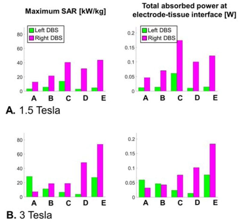
A: Unaveraged peak SAR and total absorbed power for the left and right DBS electrodes-tissue interfaces of models A, B, C, D and E simulated at 1.5 Tesla (see text for model descriptions). The total absorbed power is computed in a small cylindrical volume (diameter=10 mm, length=15 mm) surrounding the left and right lead tips (see Fig. 3C). B: Same results at 3 Tesla.

The variability of lead-tip and whole-head peak SAR and global SAR with respect to EM properties (permittivity and conductivity) variations are shown in Fig. 9 (1.5 T) and 10 (3 T). The SAR metrics at the lead-tip were computed in two small cylinders (10 mm diameter, 16 mm length) centered on the right and left DBS electrodes. SAR metrics reported for the whole head were computed in the entire body model however in which the left and right DBS leads were masked out. Whole-head SAR is usually characterized by the global SAR, not the total absorbed power, therefore for consistency we report global SAR for both the lead-tip and whole head instead of the absorbed power at the lead-tip as in Fig. 8. In this uniform body model, global SAR (GSAR) and total absorbed power (P) in the volume V are proportional:

$$\mathit{GSAR}=\frac{P}{\rho V},$$ [3]

Fig. 9.

Sensitivity of SAR predictions at 1.5 Tesla (64 MHz) with respect to variations of the conductivity and permittivity of the uniform body model. All simulations were performed using the DBS model B (full model, straight wires). First & second columns: Peak SAR and global SAR computed for 9 possible combinations of the permittivity and conductivity values for muscle, grey matter and white matter tissues at 1.5T. Third & fourth column: Variability of the peak SAR and global SAR metrics, computed as the standard deviation divided by the mean of all simulations across the parameter of interested (i.e., either the conductivity or the permittivity). A: All metrics are computed in a small cylindrical volume centered on the left and right DBS lead tips (left and right). B: All metrics are computed in the whole head, minus the left and right DBS leads.

Where ρ is the density of the medium (for human soft tissues, ρ≈1000 kg/m³). Thus the percent variability of GSAR is the same as that of P.

At the lead-tips, both peak SAR and global SAR decrease with increasing conductivity of the surrounding medium. In contrast, in the whole head these metrics increase with conductivity. This is due to the fact that the DBS lead-tip is located deep in the brain of the subject, therefore increasing the conductivity results in more and more shielding of the DBS lead-tip from the coil (this equivalent to saying that the skin depth becomes smaller and smaller, thus the total electric field, and therefore SAR, at deep locations decreases). In contrast, when considering the whole head, the locus of peak SAR is always close to the skin so that shielding is not a factor: Instead increasing the conductivity results in increased SAR because of its linear dependence on the conductivity.

At both 1.5 T and 3 T, the peak SAR and global SAR variability with respect to the conductivity was greater than that with respect to the permittivity. This is expected since SAR depends explicitly on the conductivity but only indirectly, via the electric field, on the permittivity. In addition, at both field strengths, the variability of peak SAR and global SAR with respect to the permittivity was greater around the lead-tip than in the rest of the head. This is also expected since the electrical length of the DBS implant, which has a large impact on the current induced in the lead and hence on lead-tip induced SAR, depends directly on the permittivity (increasing ε_r results in a smaller in-vivo wavelength and therefore a larger electrical length of the implant with respect to the wavelength).

In Fig. 11, we show the percent variability of absorbed power (AP, as shown in Eq. [3] the percent variety of AP is the same as that of global SAR) and peak SAR (PS in this figure) with respect to small translations (conserve the length) and scaling (does not conserve the length) of the DBS implant. At both 1.5T and 3T, the variability of AP with respect to small translations and scaling ranged from 1.0% to 8.2%. The variability of peak SAR was much greater, ranging from 19.4% to 27.6%. This is expected since the AP is an average metric that is more robust to changes in the model than peak SAR.

Fig. 11.

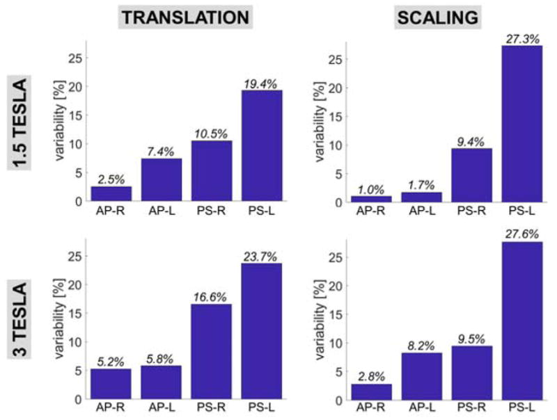
Variability of the peak SAR and absorbed power metrics with respect to +/− 1mm translation of the entire DBS implant model in the X, Y and Z directions (length is conserved) and with respect to scaling of the entire implant model (length is not conserved but does not vary more than 1 mm). All simulations were performed using the DBS model B (full model, straight wires). AP-R and AP-L mean “absorbed power, right lead” and “absorbed power, right lead”, respectively. PS-R and PS-L mean “peak SAR, right lead” and “peak SAR, left lead”, respectively.

Discussion

Simulation time

Table 2 shows processing times for each step of the proposed simulation workflow. For the patient-specific computational model used in this study, total processing time was ~11 hours. This includes DBS model generation, EM simulation at a single frequency and field export.

TABLE 2.

PROCESSING TIME FOR EACH COMPONENT OF THE SIMULATION WORKFLOW

DBS implant + uniform body model generation	~5 hours
EM simulation (model C @ 1.5 T on 13 processing cores)	Total time=259 min, solve time=150 min, peak RAM=310 GB
EM simulation (model C @ 3 T on 13 processing cores)	Total time=209 min, solve time=111 min, peak RAM=291 GB
Tuning & matching	A few seconds
Field export & conversion to Matlab format	~2 hour
TOTAL	~11 hours

Generation of the DBS implant model took ~5 hours. The bottleneck of the implant model generation was the manual reconstruction of the left and right DBS paths from the unconnected segments generated by the skeletonization algorithm (Fig. 1, STEP #4).

The use of an FEM solver for the field calculation (e.g., the HFSS solver used herein) was essential for fast simulation of the small details of the DBS implant. Using a large memory (1.5 TB), 30 processors machine, the EM simulation step was ~6 hours for all DBS models simulated in this. This is an order or magnitude faster than simulation times reported by other authors who used FDTD (the reported simulation times for this type of problem with FDTD are 24–48 hours, even when using GPU acceleration (Iacono et al., 2013; Cabot et al., 2013)).

Impact of field strength on DBS lead-tip peak SAR

For similar flip-angle distributions, we found that lead-tip peak SAR values were not generally greater at 3 T than at 1.5 T (lead-tip SAR was greater art 3 T than 1.5 T for models A, D and E; however the reverse was true for models B and C). This is against the tacit common wisdom that SAR increases monotonically with field strength. Although this may be true in patients without metallic implants, in DBS patients this “rule” is not correct because the electric length of the DBS implant relative to the in-vivo wavelength of the RF radiation is a key parameter influencing the coupling between the MRI coil and the DBS implant. This antenna effect is fundamentally a resonance mechanism, and it is not a priori obvious which frequencies (=field strength) will create a strong resonance.

Impact of model complexity on SAR

The five levels of DBS model complexity simulated in this work yielded different unaveraged peak SAR predictions. This shows the importance of detailed modeling of the DBS implant for accurate DBS-MRI safety assessment using EM simulation. For the patient simulated in this study, modeling the helicoidal geometry of the DBS internal wires (model A, as in actual implants) yielded a 1.7-fold smaller peak SAR than when modeling straight wires (model B) at 1.5 T. At 3 T, lead-tip peak SAR of the helicoidal model was 1.5-fold greater than lead-tip peak SAR in the straight model. These results are at odds with those of Cabot and al (Cabot et al., 2013), who found that tip SAR in their helicoidal wires model was ~22x smaller than in a straight-wire model. The discrepancy is likely due to the fact that the helices modeled in our study have a 2 mm pitch, which is much greater than the 0.33 mm pitch simulated by Cabot et al. Bottomley et al also found that densely wound (small pitch) helices resulted in smaller peak SAR and temperature (Bottomley et al., 2010) than loosely wound helices. If it is generally the case that tightly wound helices are associated with lower SAR, then straight wire calculations could be used as a simpler, yet conservative, simulation approach. Such a modification dramatically simplifies the EM simulation step, as modeling of tightly wound helices along the full length of the DBS implant is exceedingly difficult. A potential solution to this issue could be to simulate the DBS conductors as straight wires (as in model B), but to increase their inductance by modification of the wire diameter and/or addition of series inductor along the path. Although authors have published lumped element models (also called transmission line models) of DBS implants (Bottomley et al., 2010; Acikel and Atalar, 2011), such models do not allow modeling of the complex DBS path geometry, internal component details and the patient. Ideally, such transmission line models should be combined with FEM simulation, however it is not clear how this can be done at present.

We found that simulation of a single conductive wire for all electrodes (model C) instead of four independent wires (one for each electrode, as in model B) lead to a 1.9-fold increase in predicted peak SAR at 1.5 T and a no change at 3 T. Absence of modeling of the extension cables (model D) led to an increase in peak SAR compared to model B (1.5X at 1.5 T and 2.6X at 3 T). Finally, we found that removing the extracranial DBS loops (model E) was associated to 2.0-fold and 4.0-fold peak SAR increases at 1.5 T and 3 T, respectively (using model B as the reference). This is in agreement with previous studies by Baker et al (Baker et al., 2005) and Golestanirad et al (Golestanirad et al., 2016a) who also found that the presence of extracranial loops in the DBS path reduces peak SAR. We point out that the DBS leads in model E are not 80 cm long, as in models A, B and C (in other words, we did not uncoil the loops, but simply cut them from the model). Therefore, it is not clear whether this result (presence of extracranial loops reduces SAR and temperature) is caused by a smaller overall electrical length or the absence of extracranial loops. This relatively large variation in peak SAR values associated with the different DBS models simulated in this work suggests the need for future simulation work with more patient-specific anatomical models, DBS models, and MR RF coils. Additional models would allow for increased statistical significance and thus more robust determination of the DBS model parameters that have the most impact on SAR.

Finally, peak SAR values evaluated on the 2 mm-resolution voxel grid did not correlate well with peak SAR values evaluated on the 0.1 mm-resolution grid. This is due to significant partial voluming of the rapidly varying SAR distribution around the lead tip at 2 mm resolution, which yields unreliable estimates of peak SAR values. For stable prediction of SAR at the lead tips, we therefore used the high resolution, 0.1 mm-resolution SAR maps. This resolution was small enough to capture rapid field variations around the electrodes, but not too small that it yielded large maps difficult to work with. We point out that, in this work, the resolution of the SAR maps was not related to the FEM mesh size. As shown in Fig. 3D, the FEM mesh is an adaptive tetrahedral mesh that is very dense in regions with rapid electric field variation and less dense elsewhere – the 0.1 mm-resolution refers here to the resolution of the regular rectangular voxel grid used to export the fields for further processing of the electric field maps into SAR maps.

Comparison of SAR metrics with previous work

At 1.5 T we found the tip SAR induced around the right electrodes to be greater than SAR at the left electrodes. At 3 T, the right-lead tip SAR was greater for all models except for model A (full model, helicoidal conductors). This result is consistent with studies by Golestanirad et al (Golestanirad et al., 2016a) and Baker et al (Baker et al., 2005) which show that, in general, the presence of extracranial loops in DBS patients tend to decrease lead-tip SAR. In our model, the left electrode was closer to the IPG than the right electrode because the IPG is implanted on the left side when looking at the patient. Because the length of the left and right leads is the same, this means that the left lead needed to be coiled more than the right lead during surgery. As explained by Baker et al and Golestanirad and al, these additional loops on the left side may explain the systematically smaller lead-tip SAR on this lead.

SAR values reported in different simulations studies are exceedingly difficult to compare. This is due to the fact that different authors normalize their simulations results differently (some use unit input power excitations while other normalize the input global SAR (Angelone et al., 2010) or, like us, the average flip-angle) and use different smoothing of the SAR maps (1g, 10g, or, like in this work, no smoothing at all). Another difficulty is the fact that the SAR distribution around the DBS electrodes varies extremely quickly, therefore the spatial resolution of the SAR map used for post-processing affects dramatically the order of magnitude of the SAR values reported in different studies. Finally, at present there is no agreed way to report local SAR results for patients with DBS implants in the MRI safety community. For example, the IEC standard 60601 (Commission, 2010) is applicable to general MRI for patients without implant (in this case, the peak 10 g SAR is controlled). The ISO specification 10974 on active implantable medical device safety (ISO, 2012) explains how to compute SAR using EM simulations (4 tiers approach) but does not specify hard limits on this metric. The only limit imposed by a standard, ISO 14708 (ISO, 2017), is that the temperature increase at the lead-tip should not exceed 2 degrees. For these reasons, comparing relative trends between studies is likely much more robust than comparing absolute SAR values. We point out that this issue is one of the main reason why the MRI safety community is moving away from SAR and toward temperature limits as an end safety metric, which we plan to study in a subsequent publication.

Variability of SAR with respect to changes in EM properties and DBS implant position and length (sensitivity analysis)

Our simulations show that the variability of absorbed power (which is equal to the variability of global SAR since these two metrics are proportional) with respect to variations of the surrounding medium conductivity (σ) was 30% at 1.5T and 5% at 3T. The variability of peak SAR with respect to σ was 27% at 1.5T and 17% at 3T. These results show that the dependence of lead-tip absorbed power and peak SAR with respect to the conductivity of the surrounding medium are significant (variabilities with respect to the variations of the permittivity were smaller than 6%). Therefore, the choice of the medium conductivity in these simulations should be made carefully keeping in mind that using different values (e.g., different tissue label, different source of data for the same tissue) may have a large impact on safety predictions. We also point out that, although there is little data on this, the normal biological variability of conductivity values in healthy subjects is thought to be very large, on the order of 50% (Gabriel et al., 2009).

We also estimated the variability of the DBS lead-tip safety metrics with respect to small translations (preserves the implant length) and scaling (does not preserve the implant length) of the DBS implant model. Translations were +/− 1 mm in the X, Y and Z directions. Scaling was uniform and resulted in variations of the implant length of +/− 1 mm. We found that the variabilities of absorbed power and peak SAR were similar for both translations and scaling. For the absorbed power metric, the variability ranged from 1% to 8.2%. For the peak SAR metric, the variability ranged from 9.5% to 27.6%. This shows that the absorbed power metric is relatively robust to small changes in the implant model position and length, but that the peak SAR is not. This was expected because the absorbed power is an average metric and is naturally more robust to small changes of the model.

Taken together, these results show that the variability of lead-tip SAR results with respect to conductivity of the surrounding medium, implant position, and implant length are significant. This is especially true for the peak SAR metric, with all variabilities in the 20–30% range. The overall conclusion is to take lead-tip SAR predictions “with a grain of salt” as even a highly detailed DBS implant models may have deviations from the ground truth of more than 30%, especially when combining the different kind of variabilities studied in this work. However, although 30% variability is significant, it is still much less than the large differences observed between the SAR metrics reported for the different models in Figs. 6 and 7. As such, these differences may be significant (as explained in the next paragraph, rigorously establishing statistical significance in this case would require performing many simulations with different coil models and DBS implant geometries, instead of a single MRI coil and a single DBS patient as in this work). Finally, we point out that safety metrics based on temperature (such as peak and mean temperature in a volume of interest or the cumulative equivalent minute, CEM, metric (Sapareto and Dewey, 1984)) may be less sensitive than SAR metrics because temperature is a highly smoothed version of the SAR map.

Limitations of this work

This study shows that detailed modeling of the DBS implant, including its correct geometrical path, the presence of loops, the IPG and extension cables as well as the internal components of the implant, has a large impact on MRI-DBS safety assessment. However, in this work we simulated a single patient and a single coil configuration and therefore we do not claim that the results of Figs. 6 & 7 are applicable to the entire patient population and all scan conditions. A more comprehensive analysis would be extremely valuable for setting clinical guidelines, but would require simulation of multiple anatomical models, implant configurations, coil configurations and scan conditions (e.g., imaging landmarks) to accrue statistical significance. In fact, the large variation of SAR prediction results for the different levels of DBS implant model simplification simulated in this work is a strong motivator for performing more simulation studies with multiple patient anatomical models, DBS geometries, MR RF coils, and imaging landmarks.

Another limitation of this work is that we simulated a uniform body model truncated below the shoulders. Previous simulation work indicates that the impact of a heterogenous versus a homogeneous body model on lead-tip peak SAR is likely small (Angelone et al., 2010; Iacono et al., 2013). Because of this, we focused our investigation on the impact of DBS implant simplifications, and not on the impact of body model simplifications. The CT data used in this work can be used to segment bone and internal air structures. However, preparation of the topologically correct mesh surfaces of these complex structures ready for EM simulation within the Ansys Electronics environment is not straightforward. This is a topic we are currently working on and we will publish about in a separate publication.

Finally, we did not perform temperature modeling in this work. This would allow translation of the RF dosimetry results presented here into biologically a more relevant safety metric such as the Cumulated Equivalent Dose at 43° (Sapareto and Dewey, 1984). Doing so would also allow direct comparison of simulation and measurements of temperature at the lead tip, thus validating the whole simulation pipeline (we plan to do this in future work).

Fig. 10.

Sensitivity of SAR predictions at 3 Tesla (123 MHz) with respect to variations of the conductivity and permittivity of the uniform body model. All simulations were performed using the DBS model B (full model, straight wires). First & second columns: Peak SAR and global SAR computed for 9 possible combinations of the permittivity and conductivity values for muscle, grey matter and white matter tissues at 1.5T. Third & fourth column: Variability of the peak SAR and global SAR metrics, computed as the standard deviation divided by the mean of all simulations across the parameter of interested (i.e., either the conductivity or the permittivity). A: All metrics are computed in a small cylindrical volume centered on the left and right DBS lead tips (left and right). B: All metrics are computed in the whole head, minus the left and right DBS leads.

References

- Acikel V, Atalar E. Modeling of radio-frequency induced currents on lead wires during MR imaging using a modified transmission line method. Medical Physics. 2011;38:6623. doi: 10.1118/1.3662865. [DOI] [PubMed] [Google Scholar]
- Acikel V, Magrath P, Parker SE, Hu P, Wu HH, Finn JP, Ennis DB. RF induced heating of pacemaker/ICD lead-tips during MRI Scans at 1.5 T and 3T: evaluation in cadavers. Journal of Cardiovascular Magnetic Resonance. 2016;18:O121. [Google Scholar]
- Angelone L, Eskandaar E, Bonmassar G. Resistive tapered stripline for deep brain stimulation (DBS) leads at 7 T MRI: Specific absorption rate analysis with high-resolution head model The 24th Progress In Electromagnetics Research Symposium; 2008. p. 421. [Google Scholar]
- Angelone LM, Ahveninen J, Belliveau JW, Bonmassar G. Analysis of the role of lead resistivity in specific absorption rate for deep brain stimulator leads at 3T MRI. Medical Imaging, IEEE Transactions on. 2010;29:1029–38. doi: 10.1109/TMI.2010.2040624. [DOI] [PMC free article] [PubMed] [Google Scholar]
- Baker KB, Tkach J, Hall JD, Nyenhuis JA, Shellock FG, Rezai AR. Reduction of magnetic resonance imaging-related heating in deep brain stimulation leads using a lead management device. Neurosurgery. 2005;57:392–7. doi: 10.1227/01.neu.0000176877.26994.0c. [DOI] [PubMed] [Google Scholar]
- Bewernick BH, Hurlemann R, Matusch A, Kayser S, Grubert C, Hadrysiewicz B, Axmacher N, Lemke M, Cooper-Mahkorn D, Cohen MX. Nucleus accumbens deep brain stimulation decreases ratings of depression and anxiety in treatment-resistant depression. Biological psychiatry. 2010;67:110–6. doi: 10.1016/j.biopsych.2009.09.013. [DOI] [PubMed] [Google Scholar]
- Bonmassar G, Serano P, Angelone LM. Specific absorption rate in a standard phantom containing a Deep Brain Stimulation lead at 3 Tesla MRI. 6th International IEEE/EMBS Conference on Neural Engineering; 2013. pp. 747–50. [Google Scholar]
- Bottomley PA, Kumar A, Edelstein WA, Allen JM, Karmarkar PV. Designing passive MRI-safe implantable conducting leads with electrodes. Medical physics. 2010;37:3828–43. doi: 10.1118/1.3439590. [DOI] [PubMed] [Google Scholar]
- Cabot E, Lloyd T, Christ A, Kainz W, Douglas M, Stenzel G, Wedan S, Kuster N. Evaluation of the RF heating of a generic deep brain stimulator exposed in 1.5 T magnetic resonance scanners. Bioelectromagnetics. 2013;34:104–13. doi: 10.1002/bem.21745. [DOI] [PubMed] [Google Scholar]
- IEC 60601-2-33. Medical electrical equipment–part 2–33: Particular requirements for the basic safety and essential performance of magnetic resonance equipment for medical diagnosis 2010 [Google Scholar]
- De Coene B, Hajnal JV, Gatehouse P, Longmore DB, White SJ, Oatridge A, Pennock J, Young I, Bydder G. MR of the brain using fluid-attenuated inversion recovery (FLAIR) pulse sequences. American journal of neuroradiology. 1992;13:1555–64. [PMC free article] [PubMed] [Google Scholar]
- Denys D, Mantione M, Figee M, van den Munckhof P, Koerselman F, Westenberg H, Bosch A, Schuurman R. Deep brain stimulation of the nucleus accumbens for treatment-refractory obsessive-compulsive disorder. Archives of general psychiatry. 2010;67:1061. doi: 10.1001/archgenpsychiatry.2010.122. [DOI] [PubMed] [Google Scholar]
- Deuschl G, Schade-Brittinger C, Krack P, Volkmann J, Schäfer H, Bötzel K, Daniels C, Deutschländer A, Dillmann U, Eisner W. A randomized trial of deep-brain stimulation for Parkinson’s disease. New England Journal of Medicine. 2006;355:896–908. doi: 10.1056/NEJMoa060281. [DOI] [PubMed] [Google Scholar]
- Douglas DH, Peucker TK. Algorithms for the reduction of the number of points required to represent a digitized line or its caricature. Cartographica: The International Journal for Geographic Information and Geovisualization. 1973;10:112–22. [Google Scholar]
- Eryaman Y, Akin B, Atalar E. Reduction of implant RF heating through modification of transmit coil electric field. Magnetic Resonance in Medicine. 2011;65:1305–13. doi: 10.1002/mrm.22724. [DOI] [PubMed] [Google Scholar]
- Eryaman Y, Guerin B, Akgun C, Herraiz JL, Martin A, Torrado-Carvajal A, Malpica N, Hernandez-Tamames JA, Schiavi E, Adalsteinsson E, Wald LL. Parallel transmit pulse design for patients with deep brain stimulation implants. Magnetic Resonance in Medicine. 2014;73:1896–903. doi: 10.1002/mrm.25324. [DOI] [PMC free article] [PubMed] [Google Scholar]
- Eryaman Y, Turk EA, Oto C, Algin O, Atalar E. Reduction of the radiofrequency heating of metallic devices using a dual-drive birdcage coil. Magnetic Resonance in Medicine. 2012;69:845. doi: 10.1002/mrm.24316. [DOI] [PubMed] [Google Scholar]
- Figee M, Luigjes J, Smolders R, Valencia-Alfonso C-E, van Wingen G, de Kwaasteniet B, Mantione M, Ooms P, de Koning P, Vulink N. Deep brain stimulation restores frontostriatal network activity in obsessive-compulsive disorder. Nature neuroscience. 2013;16:386–387. doi: 10.1038/nn.3344. [DOI] [PubMed] [Google Scholar]
- Finelli DA, Rezai AR, Ruggieri PM, Tkach JA, Nyenhuis JA, Hrdlicka G, Sharan A, Gonzalez-Martinez J, Stypulkowski PH, Shellock FG. MR imaging-related heating of deep brain stimulation electrodes: in vitro study. American journal of neuroradiology. 2002;23:1795–802. [PMC free article] [PubMed] [Google Scholar]
- Gabriel C. Compilation of the Dielectric Properties of Body Tissues at RF and Microwave Frequencies. DTIC Technical Report 1996 [Google Scholar]
- Gabriel C, Peyman A, Grant E. Electrical conductivity of tissue at frequencies below 1 MHz. Physics in medicine & biology. 2009;54:4863. doi: 10.1088/0031-9155/54/16/002. [DOI] [PubMed] [Google Scholar]
- Golestanirad L, Angelone LM, Iacono MI, Katnani H, Wald LL, Bonmassar G. Local SAR near deep brain stimulation (DBS) electrodes at 64 and 127 MHz: A simulation study of the effect of extracranial loops. Magnetic Resonance in Medicine. 2016a;78:1558–1565. doi: 10.1002/mrm.26535. [DOI] [PMC free article] [PubMed] [Google Scholar]
- Golestanirad L, Keil B, Angelone LM, Bonmassar G, Mareyam A, Wald LL. Feasibility of using linearly polarized rotating birdcage transmitters and close-fitting receive arrays in MRI to reduce SAR in the vicinity of deep brain simulation implants. Magnetic resonance in medicine. 2016b;77(4):1701–1712. doi: 10.1002/mrm.26220. [DOI] [PMC free article] [PubMed] [Google Scholar]
- Greenberg BD, Malone DA, Friehs GM, Rezai AR, Kubu CS, Malloy PF, Salloway SP, Okun MS, Goodman WK, Rasmussen SA. Three-year outcomes in deep brain stimulation for highly resistant obsessive–compulsive disorder. Neuropsychopharmacology. 2006;31:2384–93. doi: 10.1038/sj.npp.1301165. [DOI] [PubMed] [Google Scholar]
- Guérin B, Gebhardt M, Cauley S, Adalsteinsson E, Wald LL. Local specific absorption rate (SAR), global SAR, transmitter power, and excitation accuracy trade-offs in low flip-angle parallel transmit pulse design. Magnetic Resonance in Medicine. 2014;71:1446–57. doi: 10.1002/mrm.24800. [DOI] [PMC free article] [PubMed] [Google Scholar]
- Guérin B, Gebhardt M, Serano P, Adalsteinsson E, Hamm M, Pfeuffer J, Nistler J, Wald LL. Comparison of simulated parallel transmit body arrays at 3 T using excitation uniformity, global SAR, local SAR and power efficiency metrics. Magnetic resonance imaging. 2015;73:1137–50. doi: 10.1002/mrm.25243. [DOI] [PMC free article] [PubMed] [Google Scholar]
- Henderson JM, Tkach J, Phillips M, Baker K, Shellock FG, Rezai AR. Permanent neurological deficit related to magnetic resonance imaging in a patient with implanted deep brain stimulation electrodes for Parkinson’s disease: case report. Neurosurgery. 2005;57:E1063. doi: 10.1227/01.neu.0000180810.16964.3e. [DOI] [PubMed] [Google Scholar]
- Hennig J, Nauerth A, Friedburg H. RARE imaging: a fast imaging method for clinical MR. Magnetic Resonance in Medicine. 1986;3:823–33. doi: 10.1002/mrm.1910030602. [DOI] [PubMed] [Google Scholar]
- Herrington TM, Cheng JJ, Eskandar EN. Mechanisms of deep brain stimulation. Journal of neurophysiology. 2016;115:19–38. doi: 10.1152/jn.00281.2015. [DOI] [PMC free article] [PubMed] [Google Scholar]
- Huff W, Lenartz D, Schormann M, Lee S-H, Kuhn J, Koulousakis A, Mai J, Daumann J, Maarouf M, Klosterkötter J. Unilateral deep brain stimulation of the nucleus accumbens in patients with treatment-resistant obsessive-compulsive disorder: Outcomes after one year. Clinical neurology and neurosurgery. 2010;112:137–43. doi: 10.1016/j.clineuro.2009.11.006. [DOI] [PubMed] [Google Scholar]
- Iacono MI, Makris N, Mainardi L, Angelone LM, Bonmassar G. MRI-based multiscale model for electromagnetic analysis in the human head with implanted DBS. Computational and mathematical methods in medicine. 2013;2013 doi: 10.1155/2013/694171. [DOI] [PMC free article] [PubMed] [Google Scholar]
- ISO/TS 10974. Assessment of the safety of magnetic resonance imaging for patients with an active implantable medical device 2012 [Google Scholar]
- ISO 14708-3. Implants for surgery -- Active implantable medical devices -- Part 3: Implantable neurostimulators 2017 [Google Scholar]
- Kozlov M, Turner R. Fast MRI coil analysis based on 3-D electromagnetic and RF circuit co-simulation. Journal of Magnetic Resonance. 2009;200:147–52. doi: 10.1016/j.jmr.2009.06.005. [DOI] [PubMed] [Google Scholar]
- Malone DA, Jr, Dougherty DD, Rezai AR, Carpenter LL, Friehs GM, Eskandar EN, Rauch SL, Rasmussen SA, Machado AG, Kubu CS. Deep brain stimulation of the ventral capsule/ventral striatum for treatment-resistant depression. Biological psychiatry. 2009;65:267–75. doi: 10.1016/j.biopsych.2008.08.029. [DOI] [PMC free article] [PubMed] [Google Scholar]
- Mayberg HS, Lozano AM, Voon V, McNeely HE, Seminowicz D, Hamani C, Schwalb JM, Kennedy SH. Deep brain stimulation for treatment-resistant depression. Neuron. 2005;45:651–60. doi: 10.1016/j.neuron.2005.02.014. [DOI] [PubMed] [Google Scholar]
- McIntyre CC, Savasta M, Kerkerian-Le Goff L, Vitek JL. Uncovering the mechanism (s) of action of deep brain stimulation: activation, inhibition, or both. Clinical neurophysiology. 2004;115:1239–48. doi: 10.1016/j.clinph.2003.12.024. [DOI] [PubMed] [Google Scholar]
- Medtronics. MRI guidelines for Medtronics deep brain stimulation systems 2015 [Google Scholar]
- Mohsin SA. Concentration of the specific absorption rate around deep brain stimulation electrodes during MRI. Progress In Electromagnetics Research. 2011;121:469–84. [Google Scholar]
- Mohsin SA, Sheikh NM, Saeed U. MRI induced heating of deep brain stimulation leads: Effect of the air-tissue interface. Progress In Electromagnetics Research. 2008;83:81–91. [Google Scholar]
- Neufeld E, Kühn S, Szekely G, Kuster N. Measurement, simulation and uncertainty assessment of implant heating during MRI. Physics in medicine and biology. 2009;54:4151. doi: 10.1088/0031-9155/54/13/012. [DOI] [PubMed] [Google Scholar]
- Park S, Kamondetdacha R, Amjad A, Nyenhuis J. MRI safety: RF-induced heating near straight wires. Magnetics, IEEE Transactions on. 2005;41:4197–9. [Google Scholar]
- Park SM, Kamondetdacha R, Nyenhuis JA. Calculation of MRI-induced heating of an implanted medical lead wire with an electric field transfer function. Journal of Magnetic Resonance Imaging. 2007;26:1278–85. doi: 10.1002/jmri.21159. [DOI] [PubMed] [Google Scholar]
- Polimeni JR, Fischl B, Greve DN, Wald LL. Laminar analysis of 7 T BOLD using an imposed spatial activation pattern in human V1. Neuroimage. 2010;52:1334–46. doi: 10.1016/j.neuroimage.2010.05.005. [DOI] [PMC free article] [PubMed] [Google Scholar]
- Puigdemont D, Pérez-Egea R, Portella MJ, Molet J, de Diego-Adeliño J, Gironell A, Radua J, Gómez-Anson B, Rodríguez R, Serra M. Deep brain stimulation of the subcallosal cingulate gyrus: further evidence in treatment-resistant major depression. Int J Neuropsychopharmacol. 2011;15:1–14. doi: 10.1017/S1461145711001088. [DOI] [PubMed] [Google Scholar]
- Sapareto SA, Dewey WC. Thermal dose determination in cancer therapy. International Journal of Radiation Oncology* Biology* Physics. 1984;10:787–800. doi: 10.1016/0360-3016(84)90379-1. [DOI] [PubMed] [Google Scholar]
- Schlaepfer TE, Cohen MX, Frick C, Kosel M, Brodesser D, Axmacher N, Joe AY, Kreft M, Lenartz D, Sturm V. Deep brain stimulation to reward circuitry alleviates anhedonia in refractory major depression. Neuropsychopharmacology. 2007;33:368–77. doi: 10.1038/sj.npp.1301408. [DOI] [PubMed] [Google Scholar]
- Serano P, Angelone LM, Bonmassar G. ISMRM. Milan, Italy: 2014. p. 4867. vol. Series 22) [Google Scholar]
- Vidailhet M, Vercueil L, Houeto J-L, Krystkowiak P, Benabid A-L, Cornu P, Lagrange C, Tézenas du Montcel S, Dormont D, Grand S. Bilateral deep-brain stimulation of the globus pallidus in primary generalized dystonia. New England Journal of Medicine. 2005;352:459–67. doi: 10.1056/NEJMoa042187. [DOI] [PubMed] [Google Scholar]
- Weaver FM, Follett K, Stern M, Hur K, Harris C, Marks WJ, Jr, Rothlind J, Sagher O, Reda D, Moy CS. Bilateral deep brain stimulation vs best medical therapy for patients with advanced Parkinson disease. JAMA: the journal of the American Medical Association. 2009;301:63–73. doi: 10.1001/jama.2008.929. [DOI] [PMC free article] [PubMed] [Google Scholar]
- Widge AS, Arulpragasam AR, Deckersbach T, Dougherty DD. In: Emerging Trends in the Social and Behavioral Sciences. Scott RA, Kosslyn SM, editors. John Wiley & Sons, Inc; 2015. [Google Scholar]
- Widge AS, Dougherty DD. Deep brain stimulation for treatment-refractory mood and obsessive-compulsive disorders. Current Behavioral Neuroscience Reports. 2015;2:187–97. doi: 10.1007/s40473-015-0036-3. [DOI] [PMC free article] [PubMed] [Google Scholar]
- Yeung CJ, Atalar E. A Green’s function approach to local rf heating in interventional MRI. Medical Physics. 2001;28:826. doi: 10.1118/1.1367860. [DOI] [PubMed] [Google Scholar]