An explainable deep machine vision framework for plant stress phenotyping

Significance

Plant stress identification based on visual symptoms has predominately remained a manual exercise performed by trained pathologists, primarily due to the occurrence of confounding symptoms. However, the manual rating process is tedious, is time-consuming, and suffers from inter- and intrarater variabilities. Our work resolves such issues via the concept of explainable deep machine learning to automate the process of plant stress identification, classification, and quantification. We construct a very accurate model that can not only deliver trained pathologist-level performance but can also explain which visual symptoms are used to make predictions. We demonstrate that our method is applicable to a large variety of biotic and abiotic stresses and is transferable to other imaging conditions and plants.

Abstract

Current approaches for accurate identification, classification, and quantification of biotic and abiotic stresses in crop research and production are predominantly visual and require specialized training. However, such techniques are hindered by subjectivity resulting from inter- and intrarater cognitive variability. This translates to erroneous decisions and a significant waste of resources. Here, we demonstrate a machine learning framework’s ability to identify and classify a diverse set of foliar stresses in soybean [Glycine max (L.) Merr.] with remarkable accuracy. We also present an explanation mechanism, using the top-K high-resolution feature maps that isolate the visual symptoms used to make predictions. This unsupervised identification of visual symptoms provides a quantitative measure of stress severity, allowing for identification (type of foliar stress), classification (low, medium, or high stress), and quantification (stress severity) in a single framework without detailed symptom annotation by experts. We reliably identified and classified several biotic (bacterial and fungal diseases) and abiotic (chemical injury and nutrient deficiency) stresses by learning from over 25,000 images. The learned model is robust to input image perturbations, demonstrating viability for high-throughput deployment. We also noticed that the learned model appears to be agnostic to species, seemingly demonstrating an ability of transfer learning. The availability of an explainable model that can consistently, rapidly, and accurately identify and quantify foliar stresses would have significant implications in scientific research, plant breeding, and crop production. The trained model could be deployed in mobile platforms (e.g., unmanned air vehicles and automated ground scouts) for rapid, large-scale scouting or as a mobile application for real-time detection of stress by farmers and researchers.

Conventional plant stress identification and classification have invariably relied on human experts identifying visual symptoms as a means of categorization (1). This process is admittedly subjective and error-prone. Computer vision and machine learning have the capability of resolving this issue and enabling accurate, scalable high-throughput phenotyping. Among machine learning approaches, deep learning has emerged as one of the most effective techniques in various fields of modern science, such as medical imaging applications, that have achieved dermatologist-level classification accuracies for skin cancer (2), in modeling neural responses and population in visual cortical areas of the brain (3), and in predicting sequence specificities of DNA- and RNA-binding proteins (4). Similarly, deep learning-based techniques have made transformative demonstrations of performing complex cognitive tasks such as achieving human level or better accuracy for playing Atari games (5) and even beating a human expert in the game Go (6).

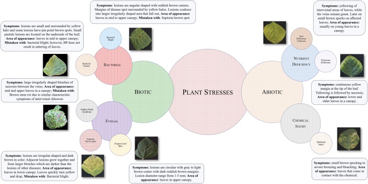
In this paper, we build a deep learning model that is exceptionally accurate in identifying a large class of soybean stresses from red, green, blue (RGB) images of soybean leaves (see Fig. 1). However, this type of model typically operates as a black-box predictor and requires a leap of faith to believe its predictions. In contrast, visual symptom-based manual identification provides an explanation mechanism [e.g., visible chlorosis and necrosis are symptomatic of iron deficiency chlorosis (IDC)] for stress identification. The lack of “explainability” is endemic to most black-box models and presents a major bottleneck to their widespread acceptance (7). Here, we sought to “look under the hood” of the trained model to explain each identification and classification decision made. We do so by extracting the visual cues or features responsible for a particular decision. These features are the top-K high-resolution feature maps learned by the model based on their localized activation levels. These features—which are learned in an unsupervised manner—are then compared and correlated with human-identified symptoms of each stress, thus providing an inside look at how the model makes its predictions.

Fig. 1.

Schematic illustration of foliar plant stresses in soybean grouped into two major categories, biotic (bacterial and fungal) and abiotic (nutrient deficiency and chemical injury) stress. The images were used to develop the DCNN for the following eight stresses: bacterial blight (Pseudomonas savastanoi pv. glycinea), bacterial pustule (Xanthomonas axonopodis pv. glycines), sudden death syndrome (SDS, Fusarium virguliforme), Septoria brown spot (Septoria glycines), frogeye leaf spot (Cercospora sojina), IDC, potassium deficiency, and herbicide injury. For each stress, information such as symptom descriptors, areas of appearance, and most commonly mistaken stresses that exhibit similar symptoms are listed. These particular foliar stresses were chosen because of their prevalence and confounding symptoms.

Materials and Methods

Leaf Sample Collection and Data Generation.

We started with the collection of images of stressed and healthy soybean leaflets in the field. The labeled data were collected following a rigorous imaging protocol using a standard camera (see SI Appendix, Sections 1 and 2 for details). Over 25,000 labeled images (https://github.com/SCSLabISU/xPLNet) were collected to create a balanced dataset of leaflet images from healthy soybean plants and plants exhibiting eight different stresses (Fig. 1). Leaflet images were taken from plants in soybean fields across the state of Iowa, in the United States. This dataset represents a diverse array of symptoms across biotic (e.g., fungal and bacterial diseases) and abiotic (e.g., nutrient deficiency and chemical injury) stresses.

Data Collection.

A total of eight different soybean stresses were selected for inclusion in the dataset, on the basis of their foliar expression and prevalence in the state of Iowa. The eight soybean stresses included the following: bacterial blight, bacterial pustule, Septoria brown spot, SDS, frog-eye leaf spot, herbicide injury, potassium deficiency, and IDC (8). Healthy soybean leaflets were also collected to ensure that the machine learning model can successfully differentiate between healthy and stressed leaves. First, various soybean fields in central Iowa associated with Iowa State University were scouted for the desired plant stresses. Entire plant samples were collected directly from the fields and taken to the Plant and Insect Diagnostic Clinic at Iowa State for official diagnosis by expert plant pathologists; for more information and online access, please follow this link to the online Plant and Insect Diagnostic Clinic (https://www.ent.iastate.edu/pidc/). The exact locations of the sampled soybean plants were recorded at that time. After the stress identities were confirmed by the Plant and Insect Diagnostic Clinic, the desired fields were revisited. Individual soybean leaflets expressing a range of severity levels were then identified and collected manually through destructive sampling. Stresses such as frogeye leaf spot, potassium deficiency, bacterial pustule, and bacterial blight were present at low to medium severity. The leaflets were placed into designated bags and taken to an on-site imaging platform.

Data Preparation and Generation.

The dataset for training, validation, and testing was prepared in the following manner: First, the images of the leaves were segmented out from the raw images (see SI Appendix, Sections 1 and 2) and reshaped into images of pixel size $64\times 64$ [(height) $\times$ (width)] for efficient training of the deep neural network. We used 4,174 images for healthy leaves, 1,511 images for bacterial blight, 1,237 images for brown spot, 1,096 images for frogeye spot, 1,311 images for herbicide injury, 1,834 images for IDC, 2,182 images for potassium deficiency, 1,634 images for bacterial pustule, and 1,228 images for SDS—that is, a total of 16,207 clean images. Refer to SI Appendix, Fig. S2 showing example images for each class.

A standard data augmentation scheme was adopted to enhance the size of the dataset. We augmented 1,096 images for each of the stress classes and augmented 2,192 images from the healthy class. The following augmentations were conducted: horizontal flip, vertical flip, 90° clockwise (CW) rotation, 180° CW rotation, and 270° CW rotation. (see SI Appendix, Fig. S3 for an illustration of the data augmentation scheme) The total dataset consisted of 65,760 images, which were then divided into training, validation, and test sets in a 7:2:1 proportion. Each image in this dataset is associated with an expert marked label indicating a stress class. For a small subset of the images ($\sim$1,000 images), we collected details of the visual symptoms that the expert pathologists used to identify a particular stress. This information was only used to quantify the explainability of the framework and was not used anywhere in the training process.

Deep CNN Model and Explanation Framework

We built a deep convolutional neural network (DCNN)-based supervised classification framework (SI Appendix, Sections 2 and 3 for details). The model (see Fig. 2) that was used for the stress identification, classification, and quantification results reported in this paper is available online (https://github.com/SCSLabISU/xPLNet). DCNNs have shown an extraordinary ability (2–6, 9, 10) to efficiently extract complex features from images and function as a classification technique when provided with sufficient data (see SI Appendix, Section 3). The exhibited accuracy is especially promising, given the multiplicity of similar and confounding symptoms between the stresses in single crop species (see Fig. 1). We associate this classification ability with the hierarchical nature of this model (11), which is able to learn “features of features” from data without time-consuming hand crafting of features (see SI Appendix, Section 2). During deployment of the model for classification inference on a leaf image, we isolate the top-K high-resolution feature maps based on their localized activation levels. These feature maps indicate regions in the leaf that the DCNN model uses to perform the classification.

Fig. 2.

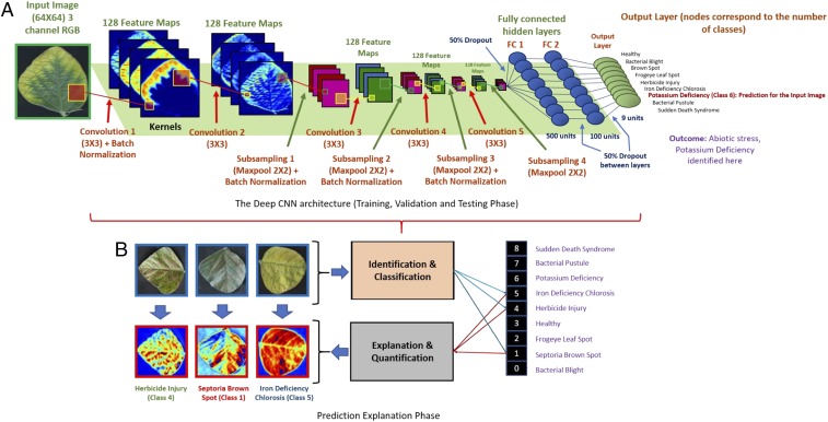
Overall schematic of the xPlNet framework: (A) DCNN architecture used. (B) Explanation phase. The concept of isolating the top-K high-resolution feature maps learned by the model based on their localized activation levels was applied to automatically visualize important image features used by the DCNN model.

Network Parameters.

After an exhaustive exploration of various applicable DCNN architectures and their classification and explanation capabilities (see detailed discussion in SI Appendix, Section 3), we choose the network shown in Fig. 2. This DCNN architecture consists of five convolutional layers ($128$ feature maps of size $3\times 3$ for each layer), $4$ pooling layers (down-sampling by $2\times 2$ max-pooling), and 4 batch normalization layers and $2$ fully connected (FC) layers with $500$ and $100$ hidden units each, sequentially. Three dropout layers were added. Two of these (with a dropout rate of $50\%$ for each) were added after each of the FC layers and another after the Flatten layer (with the same dropout rate). The learning rate was initialized with $0.001$. Training was performed using a total of $\mathrm{53,265}$ samples (with an additional $\mathrm{5,919}$ validation samples), and testing was performed on $\mathrm{6,576}$ samples. The first convolutional layer maps the three channels $(RGB)$ in the input image to $128$ feature maps by using a $3\times 3$ kernel function. Subsequent max-pooling decreases the dimensions of the image. Max-pooling is performed by taking the maximum value in the kernel window that is passed over the image. The stride here is the default stride—that is, 2—which means that the window is moved 2 pixels at a time. This decrease in image dimension not only picks up key features but also reduces computation complexity and time (12). The Rectified Linear Unit ($ReLU$) function is used as the activation function, because of significant advantages over other activation function choices. $ReLU$ increases the speed of training and requires very simple gradient computation. In the context of deep neural networks, the rectifier is an activation function, defined as $f(x)$ = $max(0,x)$, where $x$ is the input to a neuron. A unit using the rectifier is referred to as the $ReLU$. We trained the model using a NVIDIA GeForce GTX TITAN X (12 GB memory) with CUDA 8.0 (and cuDNN 5.1). See SI Appendix, Section 3 for a detailed discussion of training.

DCNN Explanation Framework for Severity Classification and Quantification.

We develop a DCNN explanation approach focused on identifying the visual cues (i.e., stress symptoms) that are used by the DCNN to make predictions. The availability of these visual cues used by the model increases our confidence in the model predictions. In this context, we observe that our DCNN model captures color-based features at the low abstraction levels (i.e., first or second convolution layer), which conforms to the general observation of deep neural networks capturing simple low-complexity but important explainable features at the lower layers (13, 14). Similarly, visual stress symptoms that a human perceives can also be described using color-based features. Therefore, these feature maps from the model can serve as indicators of visual stress symptoms as well as a means of quantifying the stress severity. We provide a brief description of our explanation approach below, with detailed mathematical formulations and algorithms available in SI Appendix, Section 4.

We begin with picking a low-level convolution layer in the model for isolating feature maps with localized activation levels. We compute the probability distribution of mean activation levels of all the feature maps for all of the healthy leaf images.* Assuming this distribution to be Gaussian, we pick a threshold (mean $+3\sigma$), called the stress activation (SA) threshold, on the mean activation levels beyond which the activation levels are considered to be indicators of a stress (similar to the notion of a reference image in explanation techniques such as DeepLIFT) (15). During inference with an arbitrary leaf image, we rank-order the feature maps at the chosen layer based on Feature Importance (FI) metric. This metric is based on the mean activation level of each feature map, computed over those pixels with activation levels above the SA threshold computed earlier. We then consider the $K$ top-ranking feature maps. We observed that most of the activation is captured by the top $2$ or $3$ feature maps among the $128$ feature maps generated at the first convolution layer (see SI Appendix, Section 4 for details). We use $K=3$ in the rest of our results. An explanation map (EM) is then generated by computing a weighted average of the top-K feature maps with the FI metrics as their weights. We find that this EM is highly correlated with the visual cues used by an expert rater to identify symptoms and quantify stress severity. Therefore, the mean intensity of the EM serves as a percentage severity level ($0\%$ being a leaf with no symptoms and a high value indicating significant symptoms), which can be discretized to provide a stress severity class. We consider a standard discretized severity scale—0% to 25%: resistant; 25% to 50%: moderately resistant; 50% to 75%: susceptible; and 75% to 100%: highly susceptible.^†

We schematically summarize the explainable deep learning framework used for plant stress identification, classification, and quantification in Fig. 2 and also provide an algorithmic summary of the overall explainable plant network (xPLNet) framework in algorithm 1.

Algorithm 1 xPlNet

• 1.Training phase: Input: $X_{train}$, $Y_{train}$: $x:$ RGB leaf images, $y:$ class labels.
• 2.Select DCNN architecture and hyperparameters.
• 3.Learn DCNN model parameters using $X_{train}$, $Y_{train}$.
• 4.Testing phase: Input: Trained DCNN model, $X_{test}$.
• 5.Compute DCNN inference for test data $\to$ Plant Stress Identification.
• 6.Explanation phase: Input: Trained DCNN model, choice of explanation layer, $X_{train}$ (only healthy leaf samples), $X_{test}$.
• 7.Generate SA threshold for the chosen explanation layer based on the healthy leaf training images.
• 8.Isolate top-K feature maps from the chosen explanation layer for the test sample using an FI metric based on localized activation levels beyond the reference SA threshold.
• 9.Generate EM via weighted averaging the top-K feature maps using the FI metric as weights.
• 10.Compute mean intensity of the EM (in grayscale) $\to$ Plant Stress Severity Quantification.
• 11.Discretize mean intensity of the EM $\to$ Plant Stress Severity Classification.

Results

Stress Identification.

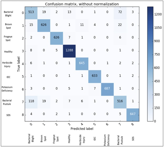
In this section, we present the results based on a DCNN model built after hyperparameter exploration that provides a good balance between high classification accuracy and explainable visual symptoms. We emphasize that the best performing model in terms of classification accuracy need not necessarily provide the best explanation (16). In Fig. 3, we present qualitative results of deploying the trained DCNN for stress identification, classification, and quantification, while quantitative results over the full test dataset are reported in Fig. 4 and Fig. 5. We found a high overall classification accuracy (94.13%) using a large and diverse dataset of unseen test examples (∼6,000 images, with around 600 examples per foliar stress). The confusion matrix revealed that erroneous predictions were predominantly due to confounding stress symptoms that cause confusion even for expert raters (Fig. 4). For example, the highest confusion (17.6% of bacterial pustule test images predicted as bacterial blight and 11.6% of bacterial blight test images predicted as bacterial pustule) occurred between bacterial blight and bacterial pustule; discriminating between these two diseases is challenging even for expert plant pathologists due to confounding symptoms (17).

Fig. 3.

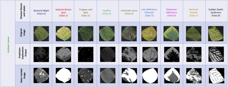
Leaf image examples for each soybean stress correctly identified by the DCNN model. The unsupervised explanation framework is applied to isolate the regions of interest (symptoms) extracted by the DCNN model, which are highly correlated (spatially) with the symptoms marked manually by expert raters.

Fig. 4.

This confusion matrix shows the stress classification results of the DCNN model for eight different stresses and healthy leaves. The overall classification accuracy of the model is 94.13%. The highest confusion among stresses was found among bacterial blight, bacterial pustule, and Septoria brown spot, which can be attributed to the similarities in symptom expression among these stresses.

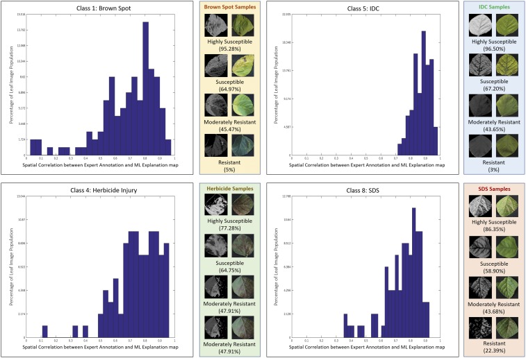
Fig. 5.

Distributions of spatial correlation between human marked symptoms and machine explanations for four stresses: Septoria brown spot, IDC, Herbicide injury, and SDS. As the distributions are significantly skewed toward high-correlation values, they show the success of the DCNN-based severity estimation framework to correctly identify symptoms for these stresses. Shown are a few examples with different severity classes (machine learning explanations on Left, actual images on Right) using a standard discretized severity scale (0% to 25%: resistant; 25% to 50%: moderately resistant; 50% to 75%: susceptible; and 75% to 100%: highly susceptible).

Symptom Explanation and Severity Quantification.

We compare the machine-based EMs with human expert ratings (which can suffer significantly from interrater variability; see SI Appendix, Section 5) by evaluating the spatial correlation function between the expert marked visual cues and the machine EM. Using the spatial correlation function compares not only total intensity but also the spatial localization of the visual cues. Fig. 5 shows the comparison using spatial correlations between the two sets of ratings (both represented in grayscale) for four different stresses (for which we had sufficient number of representative samples across various stress levels)—namely, IDC, SDS, Septoria brown spot, and Herbicide injury. Results show a high level of agreement between the machine and human ratings, which proves the viability of a completely unsupervised severity quantification technique based on an explainable DCNN framework. This allows us to avoid the very expensive pixel-level visual symptom annotations. We remind the reader that we had symptom annotations only to validate the machine-based severity ratings. We show a representative set of examples for each stress along with their EMs and human annotations in Fig. 3. The close similarity between the expert annotation with the EM significantly increases our confidence in the predictive capability of the model. We subsequently use the EMs to compute severity percentages for these examples based on mean intensities of the EMs and compute severity classes by discretizing the severity percentages as described earlier. Please see SI Appendix, Section 5 for more representative examples.^‡

High-Throughput Deployment and Transfer Learning Capability.

Well-trained DCNNs learn to generalize features rather than memorize patterns (18). We explore this characteristic and test whether the DCNN trained with a specific imaging protocol and targeted for soybean stresses could make accurate predictions under other imaging conditions and for other plant species with the same stresses. This capability for “transfer learning” (19) was investigated with several test images with IDC, Potassium deficiency, and SDS symptoms using nondestructive imaging protocols (e.g., canopy imaging with hand-held camera). With $62$ such test examples, we obtain a stress identification accuracy of $90.3\%$ (see details about the data collection strategies and test examples in SI Appendix, Section 6). Such performance of the model under different illumination conditions demonstrates the possibility of deploying this framework for high-throughput phenotyping. We also show anecdotal success for a few nonsoybean leaf image examples (e.g., IDC in cucurbits and Potassium deficiency in oilseed rape) with reasonable quality from the internet (see SI Appendix, Section 6). While such results are very promising, we refrain from drawing any firm conclusions due to the lack of availability of a statistically significant dataset of nonsoybean leaf images with stress symptoms.

Discussion

The identification of human-interpretable visual cues provides users with a formal mechanism ensuring that predictions are useful (i.e., determining whether the visual cues are meaningful). Additionally, the availability of the visual cues allows for the identification of stress types and severity classes that are underperforming (those in which the visual cues do not match the expert-determined symptoms), thus potentially leading to more efficient retraining and targeted data collection. Here, we emphasize that the identification of visual symptoms involves a completely unsupervised process that does not require any detailed rules (e.g., involving colors, sizes, and shapes) to identify the symptomatic regions on a leaf; hence, this process is extremely scalable. Furthermore, the automated identification of visual cues could be used by plant pathologists to identify early symptoms of stress. In the context of plant stress phenotyping, four stages of the problem are defined (20)—namely, identification, classification, quantification, and prediction (ICQP). In this paper, we provide a deep machine vision-based solution to the first three stages. The approach presented here is widely applicable to digital agriculture and allows for more precise and timely phenotyping of stresses in real time. We show that this approach is reasonably robust to illumination changes, thus providing a straightforward approach to high-throughput phenotyping. Similar models can be trained with data from a variety of imaging platforms and on-field protocols [unmanned aerial vehicles (UAVs), ground imaging, satellite] and various growth stages. We envision that this approach could be easily extended beyond plant stresses (i.e., to animal and human diseases) and other imaging modalities (hyperspectral) and scales (ground and air), thereby leading to more sustainable agriculture, food production, and health care.

References

- 1.Bock C, Poole G, Parker P, Gottwald T. Plant disease severity estimated visually, by digital photography and image analysis, and by hyperspectral imaging. Crit Rev Plant Sci. 2010;29:59–107. [Google Scholar]
- 2.Esteva A, et al. Dermatologist-level classification of skin cancer with deep neural networks. Nature. 2017;542:115–118. doi: 10.1038/nature21056. [DOI] [PMC free article] [PubMed] [Google Scholar]
- 3.Yamins DL, DiCarlo JJ. Using goal-driven deep learning models to understand sensory cortex. Nat Neurosci. 2016;19:356–365. doi: 10.1038/nn.4244. [DOI] [PubMed] [Google Scholar]
- 4.Alipanahi B, Delong A, Weirauch MT, Frey BJ. Predicting the sequence specificities of DNA-and RNA-binding proteins by deep learning. Nat Biotechnol. 2015;33:831–838. doi: 10.1038/nbt.3300. [DOI] [PubMed] [Google Scholar]
- 5.Mnih V, et al. Human-level control through deep reinforcement learning. Nature. 2015;518:529–533. doi: 10.1038/nature14236. [DOI] [PubMed] [Google Scholar]
- 6.Silver D, et al. Mastering the game of go with deep neural networks and tree search. Nature. 2016;529:484–489. doi: 10.1038/nature16961. [DOI] [PubMed] [Google Scholar]
- 7.Castelvecchi D. Can we open the black box of AI? Nature. 2016;538:20–23. doi: 10.1038/538020a. [DOI] [PubMed] [Google Scholar]
- 8.Koenning SR, Wrather JA. Suppression of soybean yield potential in the continental United States by plant diseases from 2006 to 2009. Plant Health Prog. 2010;10:1–6. [Google Scholar]
- 9.Sladojevic S, Arsenovic M, Anderla A, Culibrk D, Stefanovic D. Deep neural networks based recognition of plant diseases by leaf image classification. Comput Intell Neurosci. 2016;2016:1–11. doi: 10.1155/2016/3289801. [DOI] [PMC free article] [PubMed] [Google Scholar]
- 10.Ubbens JR, Stavness I. Deep plant phenomics: A deep learning platform for complex plant phenotyping tasks. Front Plant Sci. 2017;8:1190. doi: 10.3389/fpls.2017.01190. [DOI] [PMC free article] [PubMed] [Google Scholar]
- 11.Stoecklein D, Lore KG, Davies M, Sarkar S, Ganapathysubramanian B. Deep learning for flow sculpting: Insights into efficient learning using scientific simulation data. Sci Rep. 2017;7:46368. doi: 10.1038/srep46368. [DOI] [PMC free article] [PubMed] [Google Scholar]
- 12.Dumoulin V, Visin F. 2016. A guide to convolution arithmetic for deep learning. arXiv:1603.07285.
- 13.Shrikumar A, Greenside P, Kundaje A. 2017. Understanding black-box predictions via influence functions. Proceedings of the 34th International Conference on Machine Learning (ICML-17). arXiv:1703.04730v2.
- 14.Balu A, Nguyen TV, Kokate A, Hegde C, Sarkar S. 2017. A forward-backward approach for visualizing information flow in deep networks. Interpretability Symposium at the 31st Neural Information Processing Systems (NIPS-17). arXiv:1711.06221.
- 15.Shrikumar A, Greenside P, Kundaje A. Learning important features through propagating activation differences. PMLR. 2017;70:3145–3153. [Google Scholar]
- 16.Lundberg SM, Lee S-I. 2017. A unified approach to interpreting model predictions. Proceedings of the 31st Neural Information Processing Systems (NIPS-17). arXiv:1705.07874v2.
- 17.Hartman GL, et al. Compendium of Soybean Diseases and Pests. American Phytopathological Society; St. Paul: 2015. [Google Scholar]
- 18.LeCun Y, Bengio Y, Hinton G. Deep learning. Nature. 2015;521:436–444. doi: 10.1038/nature14539. [DOI] [PubMed] [Google Scholar]
- 19.Mohanty SP, Hughes DP, Salathé M. Using deep learning for image-based plant disease detection. Front Plant Sci. 2016;7:1419. doi: 10.3389/fpls.2016.01419. [DOI] [PMC free article] [PubMed] [Google Scholar]
- 20.Singh A, Ganapathysubramanian B, Singh AK, Sarkar S. Machine learning for high-throughput stress phenotyping in plants. Trends Plant Sci. 2016;21:110–124. doi: 10.1016/j.tplants.2015.10.015. [DOI] [PubMed] [Google Scholar]