Digitizing omics profiles by divergence from a baseline

Significance

Technological advances enable increasingly comprehensive profiling of the molecular landscapes of cells, and these data can inform the personalized treatment of complex diseases. Two major obstacles are the complexity of these data and the high degree of person-to-person heterogeneity. We develop a highly simplified, personalized data representation by comparing the profile of an individual to the range of landscapes in a baseline population, thereby mimicking basic clinical diagnostic testing for departures of selected variables from normal levels. Moreover, our method can be applied to any data modality and at any level of granularity, from single features to any subset of features treated as a single entity, for example the gene expression levels in a pathway. Experiments involve both healthy human tissues and various cancer subtypes.

Abstract

Data collected from omics technologies have revealed pervasive heterogeneity and stochasticity of molecular states within and between phenotypes. A prominent example of such heterogeneity occurs between genome-wide mRNA, microRNA, and methylation profiles from one individual tumor to another, even within a cancer subtype. However, current methods in bioinformatics, such as detecting differentially expressed genes or CpG sites, are population-based and therefore do not effectively model intersample diversity. Here we introduce a unified theory to quantify sample-level heterogeneity that is applicable to a single omics profile. Specifically, we simplify an omics profile to a digital representation based on the omics profiles from a set of samples from a reference or baseline population (e.g., normal tissues). The state of any subprofile (e.g., expression vector for a subset of genes) is said to be “divergent” if it lies outside the estimated support of the baseline distribution and is consequently interpreted as “dysregulated” relative to that baseline. We focus on two cases: single features (e.g., individual genes) and distinguished subsets (e.g., regulatory pathways). Notably, since the divergence analysis is at the individual sample level, dysregulation can be analyzed probabilistically; for example, one can estimate the probability that a gene or pathway is divergent in some population. Finally, the reduction in complexity facilitates a more “personalized” and biologically interpretable analysis of variation, as illustrated by experiments involving tissue characterization, disease detection and progression, and disease–pathway associations.

In recent decades, technological advances have enabled global profiling of genetic variants, RNA species, epigenetic marks, proteins, metabolites, and other previously unknown molecular features, enabling the characterization of complex biological systems over distinct molecular domains. These high-dimensional measurements have been made on thousands of samples and are collectively referred to as omics data. Through complex computational and statistical analyses of these data from different cell types and tissues, across individuals and model organisms, and from diseased and healthy conditions, we have substantially enhanced our understanding of molecular mechanisms underlying cell functioning, tissue organization, and organism development. These data are also beginning to impact clinical practice for complex diseases (1–3).

Nevertheless, omics data have yet to significantly inform the standard of care, as was expected when introduced. In part, this limitation arises from insufficient genome-wide characterization of normal variation, impeding progress toward determining whether a single omics profile reflects molecular dysregulation that is indicative of a complex disease. The use of deviation from a normal range is already widely used clinically for low-dimensional laboratory tests and biomarkers, risk assessment, disease diagnosis and prognosis, and therapy selection. Similar approaches are now needed for omics data modalities. Notably, efforts to monitor large-scale omics data in the population are now underway (4). Methods to quantify genome-wide variation, especially techniques to determine where an omics profile falls relative to a baseline, may be essential to fully realize the potential of high-dimensional omics assays; in principle, they provide unprecedented quantification of normal and disease-specific variation, which can inform clinical approaches for diagnosis and prevention of complex diseases.

To develop this high-dimensional analogue to low-dimensional clinical tests, we present a unified framework to characterize normal and nonnormal variation by quantizing high-resolution measurements into a few discrete states based on divergence from a baseline. This simplified data representation is intended to capture most of the important biological information necessary to characterize phenotypes of interest. Briefly, suppose we are given a particular subset of omics features, for example the expression levels of any set of genes; important special cases are a single gene or a functional get set. Suppose also that sample observations of this subset are available from a population declared as the baseline. Then the realization of this subset of features in any sample profile is said to be “divergent” if it lies outside the support of the baseline probability distribution. For instance, if the phenotypes of interest are cancers of a particular tissue, then a natural “baseline” population is normal samples from that tissue. However, if the goal is to determine the unique features of gene regulation in particular (normal) tissue, the baseline could be all other tissues types combined. The novelty of our framework is that it applies to any subset of features and to any new profile by itself.

Divergence is a sample property. In contrast, putative discriminating sets of features, such as “differentially expressed genes,” are defined in terms of population-level distributions. For example, given two classes or phenotypes, a gene is differentially expressed if its distribution differs in the two classes. However, knowing the status of a molecular feature in the context of populations may say very little about the status of that feature for a particular individual. Divergence then enables the prospective analysis of individual samples, as required for applications to precision and personalized medicine. It also enables a probabilistic analysis at the phenotype level, where the probability that a specific feature (say gene), or set of features (say pathway), is divergent is a well-defined concept. Phenotypes can then be characterized based on the corresponding divergence probabilities and predicted for unlabeled samples by examining the divergent set. This approach can be applied to any high-dimensional omics dataset, yielding simplified matrices of digitized values that can be analyzed statistically at the feature, sample, or phenotype level.

Deviation from a “normal” range is a form of “outlier analysis” and as such is related to other work in statistics and genomics (5–12). All of these previous studies involve single features and require standardization of a new sample with respect to multiple other samples from the same class. In contrast, divergence applies to any subprofile, and its determination does not require the availability of other samples from the same class (e.g., disease type); in fact, a new sample profile need not even be labeled. The only normalization is within-sample ranking, and all comparisons with baseline samples occur in the rank space.

Methods

The notion of “divergence” is general: Let $U$ be a random variable assuming values in a space $\mathcal{U}$ and let $P_0$ be a reference or baseline distribution on $\mathcal{U}$ with support $\text{𝑠𝑢𝑝𝑝}(P_0)\subset \mathcal{U}$. Then a value $u\in \mathcal{U}$ is divergent if $\text{𝑢}\notin \text{𝑠𝑢𝑝𝑝}(P_0)$. By definition, if $U$ has distribution $P_0$, then the probability of observing a divergent value is zero; the interest is in quantizing $U$ when it follows alternative distributions and to compare quantized values among alternatives. We are going to apply this to functions $U$ constructed from rank-normalized individual omics profiles. The supports will be estimated from data.

An omics profile is a vector $X=(X_j,j\in \mathcal{J})$ where the index set $\mathcal{J}$ and the values assumed by individual features $X_j$ depend on the particular data modality determined by the measurement technology. Typically, the features are states, counts, or concentrations of biomolecular species. In this paper, we consider gene expression (microarray and RNA-sequencing) and DNA methylation (microarray). This framework is directly applicable to other types of measurements, including single-cell data and other omics modalities (e.g., microRNA and protein expression). Here, for gene expression, $\mathcal{J}$ is the set of genes and $X_j$ is either a microarray value or RNA-seq count for gene $j$ (“bulk” mRNA); in the case of methylation, $\mathcal{J}$ is a set of CpG sites and $X_j$ is the “$\beta$ value” (see SI Appendix).

Quantiles.

In our experiments, each individual profile is transformed into quantile space: Each element of the profile is replaced by its normalized rank with respect to the other elements in the same profile. Define

$$Q_j=Q_j(X)=\frac{|\{i\in \mathcal{J}:0<X_i\le X_j\}|}{|\{i\in \mathcal{J}:0<X_i\}|}.$$ [1]

This definition returns a value $0\le Q_j\le 1$ and implies a separate treatment of ties at 0 (e.g., “nonexpressed genes”). If $X_j=0$, then $Q_j=0$, and positive quantiles are accrued only from positive $X_j$s. This is important for some data modalities, especially gene expression from RNA-seq, for which the many ties that typically occur at 0 may offset standard definitions of quantiles, assigning large quantile values to possibly small, nonzero, expression numbers. Importantly, this definition of quantiles is sample-based (i.e., they are computed across variables measured for a single subject), not population- or cohort-based.

Divergence.

Suppose we are given a reference joint probability distribution $P_0$ of $(X_j,j\in \mathcal{J})$ associated with some baseline phenotype. Of course, in practice, we only observe samples from this distribution where each sample is an omics profile from a single data modality, and the choice of reference phenotype depends on the particular study and data modality. As will be seen in Results, the baseline phenotype need not be a single tissue type or a disease-free phenotype and can be any population that is meaningful under the analysis carried out.

Given an omics profile $X$ and a subset $S\subset \mathcal{J}$, we will apply the definition of divergence to the random vector $U^S=Q^S(X)=(Q_j(X),j\in S)$. We will focus on single features $S=\{j\}$ (e.g., single genes) and on sets $S$ with $1\ll |S|\ll |\mathcal{J}|$ (e.g., gene pathways). Let $m=|S|$, so that $U^S$ takes values in ${[\mathrm{0,1}]}^m$. We describe below how the support ${\mathcal{U}}_0^S\subset {[\mathrm{0,1}]}^m$ of $U^S$ can be estimated from the data, resulting in a set ${\widehat{\mathcal{U}}}_0^S$ that is explicitly defined. When presented with a new sample $X$, we define a binary variable by

$$Z=\{\begin{array}{cc}\hfill 1& \text{if}\hspace{0.17em}{Q}^S(X)\notin {\widehat{\mathcal{U}}}_0^S,\hfill \\ \hfill 0& \text{otherwise}.\hfill \end{array}$$

We will then say that the set $S$ is divergent (for the considered sample) if and only if $Z=1$.

Support Estimation.

The support of the random vector $U^S=Q^S(X)$ under $P_0$ is estimated by a “covering” of the observed baseline samples. Covering methods for the estimation of the support of a multivariate density were introduced in ref. 13, with a goal similar to ours of detecting abnormal behavior. The estimator ${\widehat{\mathcal{U}}}_0^S$ that we propose is a variation of the one proposed in that paper. Let $d$ be a metric on ${[\mathrm{0,1}]}^m$ (we will use the Euclidean distance). Assume that $n_0$ independent and identically distributed (i.i.d.) samples of $X$ are observed under $P_0$, resulting in i.i.d. samples $U^S(1),\mathrm{\dots },U^S(n_0)$; these are now $n_0$ points in ${[\mathrm{0,1}]}^m$. We will define an increasing sequence of empirical supports indexed by a “smoothing” parameter $\gamma \in [\mathrm{0,1}]$; the determination of $\gamma$ is described later. Let $l=l(\gamma )=[\gamma n_0]$, the greatest integer less than or equal to $\gamma n_0$. For each $k\in \{1,\mathrm{\dots },n_0\}$, let $r_k$ denote the distance between $U^S(k)$ and its $l$th nearest neighbor. We define

$${\widehat{\mathcal{U}}}_0^S={[\mathrm{0,1}]}^m\cap \bigcup _{k=1}^{n_0}B(U^S(k),r_k),$$ [2]

where $B(U^S(k),r_k)$ denotes the closed ball of center $U^S(k)$ and radius $r_k$. In other terms, a point $u\in {[\mathrm{0,1}]}^m$ belongs to ${\widehat{\mathcal{U}}}_0^S$ if and only if there exists $k\in \{1,\mathrm{\dots },n_0\}$ such that $U^S(k)$ is closer to $u$ than to its $l$th nearest neighbor. The smoothing parameter $\gamma$ corresponds to the “bandwidth” in multivariate density estimation (14), and our estimator, based on nearest neighbor distances, implements what is commonly referred as an “adaptive bandwidth” method in this literature.

The estimate of the support in Eq. 2 is very conservative: Every subprofile $S$ is nondivergent for every sample from the baseline population. This is unrealistic, not only in view of possible outliers among the baseline samples, but also because these baseline samples may in fact contain a small proportion of nonbaseline cell types. Another drawback is that $\gamma$ is yet to be specified. We address these two issues simultaneously. Again, let $r_1,\mathrm{\dots },r_{n_0}$ be the radii of the balls centered at baseline samples. Now let $\overline{r}$ be the $95$th percentile of these radii. Instead of covering all of the baseline samples, we remove the $5\%$ for which $r_k>\overline{r}$ before computing the support. That is, the support is constructed as in Eq. 2 but with the union over all $k=1,\mathrm{\dots },n_0$ replaced by the union over $\{k:r_k\le \overline{r}\}$. Notice that some “left-out” samples may still lie in the support, but in general some will not, and therefore, some features will be declared divergent for some baseline samples. The smaller is $\gamma$, the more baseline divergence.

For $m=1$, say $S=\{j\}$, the estimated support is simply a union of intervals centered at the quantile values of a subset of baseline samples with interval lengths determined by $\gamma$. In nearly all cases of interest, this union is itself an interval; that is, there are no “gaps.” Making this assumption (or replacing the support by its convex hull), it suffices to compute its upper and lower bounds. This can be done by first computing the smallest and largest values among the (retained) baseline samples $U^j(k)$ for $r_k\le \overline{r}$, denoted respectively by $m_j$ and $M_j$, and then estimating the baseline support of feature $j$ by ${\widehat{\mathcal{U}}}_0^j=[l_j^0,u_j^0]\subset [\mathrm{0,1}]$, where $l_j^0=\max (0,m_j-d_1)$ [respectively, $u_j^0=\min (1,M_j+d_2)$] and $d_1$ (respectively, $d_2$) is the distance from the smallest sample (respectively, the largest) to its $l$th nearest neighbor among the retained baseline samples.

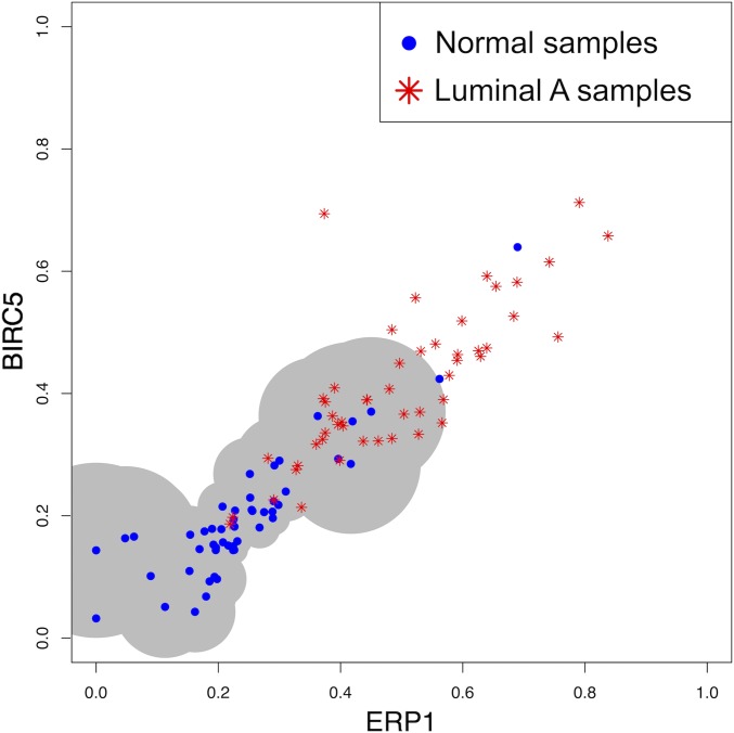
An example of the estimated support for two genes ($|S|=2$) and $\gamma =.1$ is shown in Fig. 1. The data are gene expression values for 50 samples of normal breast tissue, and the two genes—“ERP1” and “BIRC5”—are clearly correlated. Since there are $n_0=50$ normal samples, the estimated support is the union of 47 disks, where the radius of the disk centered at each pair of quantile values is the Euclidean distance to its fifth nearest neighbor ($[.1(50)]=5$). The extent of coverage obviously depends on $\gamma$.

Fig. 1.

2D baseline support. Fifty normal samples (blue points) and 50 luminal A samples (red stars) were chosen at random from The Cancer Genome Atlas (TCGA) breast cancer data. The area of support computed using the normal samples is shown by the gray shade; the samples falling outside the support are declared divergent.

We will apply the definition of divergence in two scenarios: (i) All single features are considered, so divergence is determined for $S=\{j\}$ for every $j\in \mathcal{J}$; (ii) divergence is applied to collections of sets $S_1,\mathrm{\dots },S_N$—for example, pathways or functional gene sets (FGSs)—where the sets may be overlapping and of different dimensions. In our experiments, we use FGSs retrieved from the Broad Institute Molecular Signature Database (MSigDB) (15). The divergent set is denoted by $𝐃(X)=\{j:Z_j\ne 0\}$, where $𝐃\subset \mathcal{J}$ in case i and $𝐃\subset \{1,\mathrm{\cdots },N\}$ in case ii. In all cases, $𝐃$ is a random set—that is, is sample-dependent. For single features, where the supports are intervals $[l_j^0,u_j^0]$, the definition can be refined:

$$Z_j=\{\begin{array}{cc}-1,\hfill & \text{if}{Q}^j(X)<l_j^0\hfill \\ \mathrm{\hspace{0.17em}\hspace{0.17em}1},\hfill & \text{if}{Q}^j(X)>u_j^0\hfill \\ \mathrm{\hspace{0.17em}\hspace{0.17em}0},\hfill & \text{otherwise}\hfill \end{array}.$$

We will then say that $j$ is lower divergent if $Z_j=-1$ and upper divergent if $Z_j=1$, and let ${𝐃}^l(X)=\{j:Z_j=-1\}$ and ${𝐃}^u(X)=\{j:Z_j=1\}$ denote the set of lower divergent and upper divergent features.

Parameters.

Returning to the choice of $\gamma$, a natural way to control the level of baseline divergence is to limit on the average fraction $\alpha$ of divergent features in the baseline population, namely $E_0\left(\frac{|𝐃|}{M}\right)$, where $M=|\mathcal{J}|$ for single features and $M=N$ for a family of $N$ subsets. We then select the smallest $\gamma$, which achieves this fraction $\alpha$, where the same $\gamma$ is used for every support estimator. Therefore, once $\alpha$ is fixed, there are no other parameters to specify. This is because $\alpha$ determines $\gamma$ and $\gamma$ determines the radii $r_1,\mathrm{\dots },r_{n_0}$, which in turn determine the estimated supports. In our experiments with single-feature divergence, we select $\alpha \equiv .01$; with functional gene sets, we take either $\alpha =.01$ or $\alpha =.001$ (see Results).

Results

Divergence of Tumor Profiles from a Normal Baseline.

We measured $|𝐃|$, the degree of divergence, for single features in gene expression (microarray and RNA-seq) and DNA methylation profiles of tumor samples from various tissues, using the corresponding normal counterpart as the baseline. We also measured $|𝐃|$ at the gene set level using data from The Cancer Genome Atlas (TCGA) (16) and the MSigDB Hallmark FGS collection; again, the baseline is normal tissue. As described in Methods, for any given sample profile, a set of features $S$ is defined as divergent if the assumed quantile value(s) fall outside the estimated baseline support.

In measuring the extent of divergence in tumor samples, for each tissue and omics data type, half of the available normal samples were randomly selected to estimate the baseline support. Then divergence was determined for the left-out normal and all tumor samples (see SI Appendix, Methods for details).

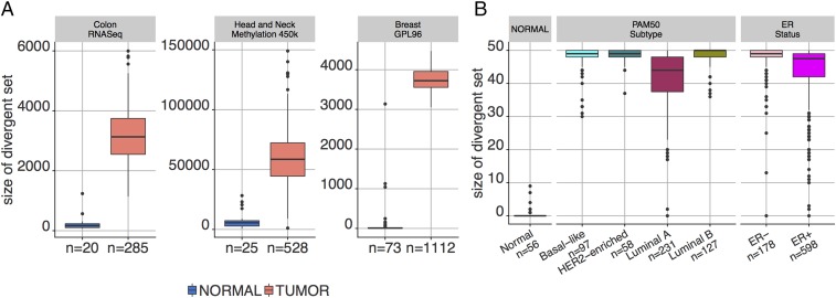
Overall, for single features, typically thousands are divergent in tumors for both gene expression and DNA methylation, irrespective of the platform used to generate the data and the tissue type. In all cases, the difference in the level of divergence between normal and tumor samples in each tissue and platform cohort is highly significant (Wilcoxon P value < ${10}^{-6}$; see Fig. 2). In fact, the differences in $|𝐃|$ are sufficiently large to allow for near-perfect separation without even taking into consideration the identity of the features in $𝐃$. Similar results were also obtained for additional tumor types, as measured by RNA-seq in TCGA or using other microarray platforms (see SI Appendix, Fig. S1 A–C). The same pattern persisted when the divergent set $𝐃$ was replaced by the upper and lower divergent sets ${𝐃}^u$ and ${𝐃}^l$.

Fig. 2.

Degree of divergence in tumor and normal sample populations. (A) Single features for RNA-seq gene expression, CpG methylation, and microarray expression. (B) The 50 FGSs in MSigDB “Hallmark” collection. Note that, by design, the level of divergence in the normal populations is extremely small. In both cases, divergence is learned from a separate normal population.

Turning to the divergence of gene sets, the divergent set $𝐃$ is now a sample-specific set of pathways. For the breast cancer subtypes, the sizes $|𝐃|$ for our TCGA samples are shown in Fig. 2B. As with single features, this sample statistic appears to be highly discriminating in separating normal and tumor samples. In fact, training a linear support vector machine (SVM) classifier (effectively just thresholding the size of $𝐃$) on half the data from each group and testing on the other half yields test accuracies $99.2\%,100\%,100\%,100\%,98.3\%,99.5\%$, respectively, for normal vs. luminal A, luminal B, basal-like, HER2-enriched, ER+, and ER– tumors.

Probabilities of Divergence Across Populations.

We estimated the probability $P(Z_j=1|Y=y)=P(j\in 𝐃|Y=y)$ that a sample from phenotype $y$ is divergent. We did this both for single features $j$ and for gene sets $S_j$, and for both breast cancer molecular subtypes in TCGA and a large variety of normal samples from distinct tissue types obtained from the GTEx project (17). All probability estimates are relative frequencies in training data.

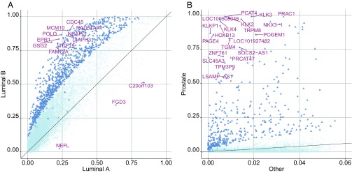
For single features, we compared ternary feature-level divergence profiles between luminal A and luminal B breast cancer. For most genes, luminal B samples are more likely to be divergent than luminal A tumors. In particular, almost all of the genes identified as significantly “differentially divergent” (${\chi }^2$ test, Bonferroni corrected P value $\le 0.05$) and had higher probabilities of divergence in luminal B (see Fig. 3A). Of note, our finding of a greater degree of dysregulation (i.e., greater divergence from the baseline) associated with luminal B is consistent with the more aggressive behavior of this subtype compared with luminal A, characterized by multiple factors portending a poorer prognosis, including higher grade, larger size, and spreading to lymph nodes (18–20).

Fig. 3.

Differentially divergent genes between tumor phenotypes. (A) Scatter plot of divergence probabilities of genes for 231 luminal A and 127 luminal B breast cancer samples in TCGA. After Bonferroni correction, 941 genes (blue triangles) have an adjusted P value $\le 0.05$ for a ${\chi }^2$ test comparing the two subtypes using ternary digitized data. Among these, the genes with the smallest P values are labeled. (B) Scatter plot of divergence probabilities of genes for 106 prostate and 4216 nonprostate samples in Genotype-Tissue Expression (GTEx) with respect to a nonprostate baseline. After Bonferroni correction, 433 genes (blue triangles) have an adjusted P value $\le 0.05$ in a ${\chi }^2$ test comparing the two groups. The 20 genes with the smallest P values and higher divergence probability in prostate are labeled.

We also analyzed RNA-Seq data from GTEx to identify genes showing highly tissue-specific expression patterns. To this end, we compared divergence probabilities between a given normal tissue of interest, say $T$, and the remaining ones. First, we computed a multitissue baseline profile from 50% of available non-$T$ samples, and then, estimated divergence probabilities separately from all of the $T$ samples and the remaining half of non-$T$ samples. For example, to identify prostate-specific genes, we used half of nonprostate samples pooled together to estimate a nonprostate baseline. This analysis yielded 433 prostate-specific significant genes (Bonferroni-adjusted P value $\le 0.05$), encompassing many known prostate markers including KLK3 (a.k.a. the prostate specific antigen; see Fig. 3B). Then, we reversed the roles: We took tissue $T$ as the baseline, with support estimated from 50% of the $T$ samples and probabilities estimated as described above. This reverse approach also identified phenotype-specific genes (see SI Appendix, Figs. S2 and S3).

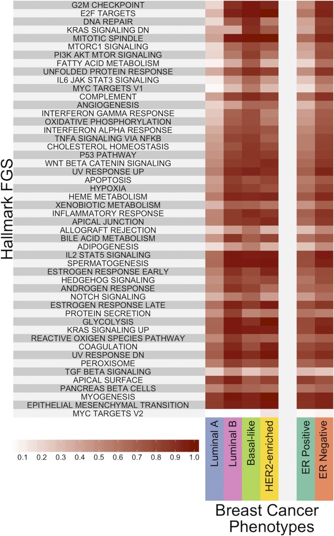
For gene sets, we considered the breast cancer subtypes and the 50 Hallmark gene sets. Since we are estimating only a limited number of supports, we imposed virtually zero normal divergence by selecting $\alpha =.001$, with the risk of underestimating cancer subtype divergence probabilities if in fact the normal breast samples are contaminated. Fig. 4 shows a heat map of the probabilities of divergence for each of the 50 pathways. The full table of values is in SI Appendix, Table S1.

Fig. 4.

Divergent probabilities for Hallmark FGSs. The heat map shows the divergence probabilities, as coded in the color scheme above, for the Hallmark FGS collection across breast cancer phenotypes.

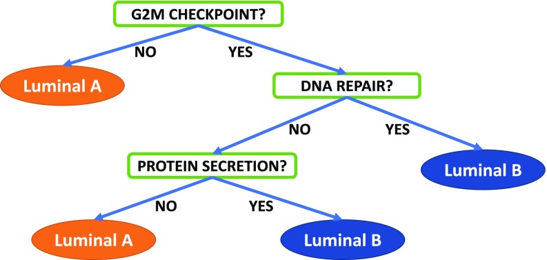
In addition, given the large differences in divergent probabilities observed among subtypes for certain pathways, we built a single decision tree to distinguish between luminal A and luminal B subtypes using half the samples for learning the tree and the other half for estimating the accuracy. Each question in the tree is of the form “Is pathway X divergent?”, where $X$ can be any of the 50 hallmark pathways. This experiment in classification is merely an illustration of the different types of analysis that can be performed within our framework; more accurate trees could be induced by regarding $\alpha$ as a parameter to be optimized in cross-validation. Notice the considerable gain in interpretability that can be achieved with multidimensional divergence relative to black box predictors: Even using only three pathways, the test accuracy is $81\%$ (see Fig. 5).

Fig. 5.

Decision tree for separating luminal A and B breast cancer subtypes. For each individual sample, the answer to the question is “YES” if the indicated pathway (e.g., “G2M CHECKPOINT”) is divergent and “NO” otherwise.

Comparing Divergence Profiles Across Tissue Types.

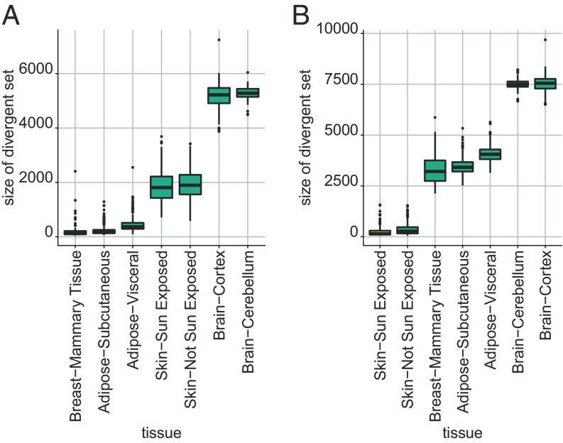
We also used the GTEx data to compare normal samples across tissue types. For each tissue, we randomly selected half of the samples as the baseline and then computed the divergence sets for the left-out samples from the same tissue as well as all of the samples from other tissues. Fig. 6 shows the results obtained for two tissue subtypes used as the baseline (breast and skin) on a selection of seven tissue subtypes. As expected, in all cases, the remaining samples of the tissue subtype declared as the baseline showed the least divergence, while the samples from the different subtypes displayed varying degrees of divergence; SI Appendix, Fig. S4 shows additional results with the full list of available GTEx tissues.

Fig. 6.

Divergence profile comparison between normal tissue types. Using (A) breast and (B) sun-exposed skin tissue as baselines, divergence sets are computed for multiple normal tissue subtypes available in GTEx with RNA-seq gene expression profiles. Half of the available samples were used to estimate a normal subtype-specific profile, and the divergence of all remaining samples was computed with respect to this baseline.

The relative degrees of divergence depend on how related the tissue types are Samples from other tissues that share common cell types with the baseline have fewer divergent features (e.g., breast and adipose tissue in Fig. 6A) than those that do not (e.g., skin and brain in Fig. 6B). This suggests that tissue-specific gene expression baselines could be used to predict the tissue type of samples of unknown type. To test this hypothesis, we analyzed 48 tissue types in GTEx, deriving tissue-specific baselines using 50 randomly selected samples from each tissue type and then classifying the tissue-type of the remaining samples. A sample is classified as the tissue type that provides the smallest number of divergent genes. In general, accuracies above 90% were observed. Moreover, incorrect predictions of tissue type always reflected cell type composition and tissue origin. For instance, the fact that virtually all misclassified breast samples were labeled as adipose tissue might be expected since the mammary glands contain substantial amounts of adipose cells. Similarly, different regions of the brain share the same embryological origin and cellular types (see SI Appendix, Fig. S5).

Comparison of Divergence Profiles Between Disease Phenotypes.

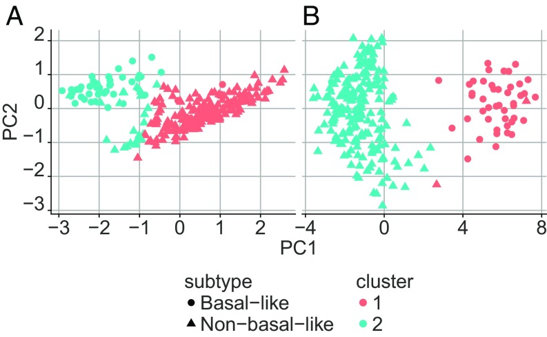
Next, we considered the effect of the divergence transform on unsupervised learning. In particular, we compared the results of spectral clustering for the quantile data and the ternary data. As above, all normal (baseline) and tumor samples were taken from TCGA, and the mean fraction of normal divergence was controlled at $\alpha =.01$ relative to the entire transcriptome. Samples were randomly and evenly divided into training and test. Based on the training data, we determined the 100 most differentially expressed genes for the four breast cancer subtypes (luminal A, luminal B, HER2-enriched, and basal-like); we used the Kruskal–Wallis test for the quantile data and the ${\chi }^2$ test for the ternary data. We applied spectral clustering to the aggregated training data, both quantile and ternary. In both cases, we obtain two major, well-separated clusters, one dominated by basal-like samples and the other by non–basal-like samples (see Fig. 7). Clearly, by this criterion, the discriminating information is retained in the divergence profiles.

Fig. 7.

Clustering digitized data. Results of spectral clustering of Breast TCGA RNA-seq data in (A) quantile form and (B) digitized form. The resulting clusters discriminate basal-like samples from all other subgroups. Digitized data preserve biological information separating the different subtypes similarly to quantile data.

Furthermore, we compared divergence profiles across multiple clinically relevant, and progressively more pathogenic, cancer phenotypes. This revealed an increasing trend in average divergence from the normal baseline, strongly suggesting that divergence analysis can efficiently capture the global dysregulation associated with cancer progression or risk factor exposure. For instance, gene expression divergence increased in prostate cancer with increasing Gleason grade: the average size of the divergent set was $883$ for tumors with a primary Gleason grade of 3, $1241$ for a primary Gleason grade of 4, and $1490$ for a primary Gleason grade of 5. Similar results were also observed in breast cancer with increasing grade, in the progression from colon adenoma to carcinoma, and for DNA CpG methylation divergence in lung cancer, which increased with tobacco-smoke exposure (see SI Appendix, Fig. S6 A–D). Notably, the level of deviation from the normal baseline is strongly correlated between distinct omics modalities derived from the same biological samples, suggesting global genome-wide dysregulation in both DNA and RNA in cancer; see, for example, the case of prostate cancer gene expression and methylation in SI Appendix, Fig. S7A (Spearman correlation $0.59$). Repeating this analysis with breast cancer data yielded a Spearman correlation of $0.51$ (SI Appendix, Fig. S7B). Overall, these results suggest that the divergence framework is capturing a sparse yet biologically meaningful snapshot of an omics sample and its dysregulation from a healthy state, which can be observed across distinct omics data modalities.

Discussion

Combing through large datasets to make meaningful biological inferences has become the raison d’être for much of the current work in bioinformatics. Often the goal is the discovery of biomarkers or molecular signatures (e.g., gene sets) of clinical utility, and a great many of these based primarily on gene expression have been proposed over the last 15 years. However, many high-throughput omics classifiers are learned from relatively small cohorts of samples using population-level estimates that are highly sensitive to variability, and therefore, the resulting biomarkers are often difficult to reproduce and validate (21–23). As a result, leveraging such “gene signatures” has proven difficult; in fact, the majority of such biomarkers are unable to meet the rigorous criteria required to be admitted to clinical use. The work here is aimed at ameliorating some of these barriers.

Sensitivity to platform and preprocessing is one important barrier. Divergence coding begins with the initial conversion of raw feature values to within-sample ranks to minimize preprocessing and batch effects. This is also the first step in “quantile normalization” (24) and in the work on “relative expression analysis.” The latter includes the top scoring pair (TSP) and k-TSP algorithms for distinguishing between two disease phenotypes based on the expression ordering between two genes (25) and between k pairs of genes (26, 27), as well as the “RankComp” approach (28), which aims at identifying dysregulated gene pairs starting from a pool of stable pairs precompiled using normal samples. Within-profile rank normalization was extended to “differential variation” between pathways using Hamming distance to a phenotype-specific rank template (29) and using the Kendall-tau or “swap” distance between rank vectors (30, 31).

Concerning “outliers” in omics data, an early example is “Cancer Outlier Profile Analysis” (COPA) (6, 7) for gene expression: First, each gene is standardized across samples from a phenotype of interest, and then those genes that display an outlier profile over a subset of samples are selected. This COPA framework can also be extended to model heterogeneity in integrated data modalities, and separate gene set statistics can be applied to determine whether outliers are enriched in multidimensional gene sets (11).

All of the current methods to quantify dysregulation require prior knowledge of the sample phenotypes and a population of samples from each phenotype. Divergence is a sample-level property that can be applied to a single sample without knowledge of phenotype and thus is not directly comparable to these methods. The approach perhaps most closely related to divergence is the “Anti-Profiles” method introduced in refs. 10, 32 and applied to cancer diagnosis; genes that deviate from a normal profile are identified after standardization across samples and after prefiltering for hypervariability with respect to normal samples. In contrast, our method requires no across-sample standardization or prefiltering, making it amenable to the analysis of individual samples prospectively collected. Moreover, similar to outlier analysis, the antiprofile approach requires subsequent set statistics for pathway analysis. Divergence applies to any subset of features treated as a single entity using the same statistical theory. Both of these differences further limit direct comparison of divergence to the antiprofile approach.

Enormous biological variation is another barrier. It has been consistently observed that in many disease conditions there is a high degree of variation in the omics profiles from sample to sample. Observations of individual samples and genomic features at high-resolution may obscure patterns of dysregulation. Furthermore, omics studies usually focus on population-level statistics derived from samples from two or more classes. The features measured (e.g., transcript levels, CpG methylation) are treated as random variables, and properties of their distributions are estimated from the data and compared between classes of interest. For instance, statistical testing is used to identify a set of genes for which the marginal distribution is significantly altered from one phenotype to another. In contrast, in the work here, “differential expression” is a sample property.

Estimating of the support of a distribution in high dimensions with unions of balls is a complex problem; in particular, the accuracy will depend heavily on the “effective” number of dimensions. When the data are supported by a neighborhood of a small-dimensional manifold of a large-dimensional space, our support estimator will be much more likely to resemble the ground truth. Preliminary experiments suggest that this is indeed the case, but this topic requires further study.

When using a small number of baseline samples, our definition of divergence will definitely lack precision and, because of large interpoint distances, will probably err on the side of being overconservative, with a corresponding loss of power. However, our results show that the divergence signal is so strong in cancer that even being overconservative allows for a large number of out-of-support samples. A loss of power might also result from analyzing high-dimensional subsets of features. A related issue is the complexity of the baseline distribution, especially how to accommodate heterogeneous baseline populations. Such populations may require refinements such as linking divergence to covariates. This issue will also be the subject of future research.

Finally, the complexity and black box nature of many bioinformatics methods often prevents reconciling the statistical findings and decision rules with any underlying biological mechanism. In contrast, capturing and quantifying the deviation of a disease sample from the normal, physiologic state is directly meaningful, inherently interpretable, and well-suited for applications to precision and personal medicine, including clinical risk assessment and therapy selection.

Conclusion

The concept of divergence from a baseline requires making robust and meaningful comparisons from profile to profile. Here, we begin by converting every raw profile of interest to a quantile space by normalizing within-sample ranks. Then, given sufficiently many samples from a suitable baseline population, defining divergence boils down to the ability to estimate the support of the underlying baseline probability distribution. Importantly, divergence labeling of any given sample requires no further standardization with respect to other samples of the same class. Estimation of the baseline support is straightforward for scalar random variables such as individual omics features (e.g., the expression of a single gene) since the baseline support is simply an interval; for random vectors assuming values in an m-dimensional space (e.g., the expression of all genes in a pathway), we have estimated the support using a metric-based covering argument. In both cases, by construction, the divergence transform provides a massive reduction in complexity. We have demonstrated that, nonetheless, a great deal of important biological information is preserved.

We have focused on applications to human disease, primarily cancer. The emphasis on patient-level molecular dysregulation is in line with many accepted paradigms of pathogenesis. Cancer is particularly subject to such molecular heterogeneity. Stimulating cell proliferation, inducing abnormality in metabolic pathways, and genome instability are considered to be hallmarks of cancer progression and can collectively, along with many of the remaining hallmarks, be considered dysregulation of normal cell behavior. Therefore, a method that can quantify the presence of dysregulation in a disease sample is directly meaningful and appropriate for assessing risk.

The analytical framework presented here could be applied to the study of other complex human diseases that display high levels of interpersonal heterogeneity. As shown here with cancer, we expect that genomic and epigenomic divergence are pervasive and that the extent of divergence is often associated with relative gravity. Future work will center on the major challenge of adapting a patient-level divergence profile to individualized patient care.

Data and Code Availability

All data analyzed here are available from luigimarchionni.org/divergence.html, and the necessary packages and code can be obtained from github.com/wikum/DivergenceAnalysis.

References

- 1.Li Xj, et al. A blood-based proteomic classifier for the molecular characterization of pulmonary nodules. Sci Transl Med. 2013;5:207ra142. doi: 10.1126/scitranslmed.3007013. [DOI] [PMC free article] [PubMed] [Google Scholar]
- 2.Ross AE, et al. Tissue-based genomics augments post-prostatectomy risk stratification in a natural history cohort of intermediate- and high-risk men. Eur Urol. 2016;69:157–165. doi: 10.1016/j.eururo.2015.05.042. [DOI] [PubMed] [Google Scholar]
- 3.Saade GR, et al. Development and validation of a spontaneous preterm delivery predictor in asymptomatic women. Am J Obstet Gynecol. 2016;214:633.e1–633.e24. doi: 10.1016/j.ajog.2016.02.001. [DOI] [PubMed] [Google Scholar]
- 4.Price ND, et al. A wellness study of 108 individuals using personal, dense, dynamic data clouds. Nat Biotechnol. 2017;35:747–756. doi: 10.1038/nbt.3870. [DOI] [PMC free article] [PubMed] [Google Scholar]
- 5.Parmigiani G, Garrett-Mayer ES, Anbazhagan R, Gabrielson E. A statistical framework for expression-based molecular classification in cancer. J R Stat Soc Ser B Stat Methodol. 2002;64:717–736. [Google Scholar]
- 6.Tomlins SA, et al. Recurrent fusion of TMPRSS2 and ETS transcription factor genes in prostate cancer. Science. 2005;310:644–648. doi: 10.1126/science.1117679. [DOI] [PubMed] [Google Scholar]
- 7.Tibshirani R, Hastie T. Outlier sums for differential gene expression analysis. Biostatistics. 2006;8:2–8. doi: 10.1093/biostatistics/kxl005. [DOI] [PubMed] [Google Scholar]
- 8.Zilliox MJ, Irizarry RA. A gene expression bar code for microarray data. Nat Methods. 2007;4:911–913. doi: 10.1038/nmeth1102. [DOI] [PMC free article] [PubMed] [Google Scholar]
- 9.McCall MN, Uppal K, Jaffee HA, Zilliox MJ, Irizarry RA. The gene expression barcode: Leveraging public data repositories to begin cataloging the human and murine transcriptomes. Nucleic Acids Res. 2011;39:D1011–D1015. doi: 10.1093/nar/gkq1259. [DOI] [PMC free article] [PubMed] [Google Scholar]
- 10.Dinalankara W, Bravo HC. Gene expression signatures based on variability can robustly predict tumor progression and prognosis. Cancer Inform. 2015;14:71–81. doi: 10.4137/CIN.S23862. [DOI] [PMC free article] [PubMed] [Google Scholar]
- 11.Ochs MF, et al. Outlier gene set analysis combined with top scoring pair provides robust biomarkers of pathway activity. In: Ngom A, Formenti E, Hao JK, Zhao XM, van Laarhoven T, editors. Pattern Recognition in Bioinformatics. Springer Berlin Heidelberg; Berlin: 2013. pp. 47–58. [Google Scholar]
- 12.Afsari B, Geman D, Fertig EJ. Learning dysregulated pathways in cancers from differential variability analysis. Cancer Inform. 2014;13:61–67. doi: 10.4137/CIN.S14066. [DOI] [PMC free article] [PubMed] [Google Scholar]
- 13.Devroye L, Wise GL. Detection of abnormal behavior via nonparametric estimation of the support. SIAM J Appl Math. 1980;38:480–488. [Google Scholar]
- 14.Scott DW. Multivariate Density Estimation: Theory, Practice, and Visualization. John Wiley & Sons; Hoboken, NJ: 2015. [Google Scholar]
- 15.Liberzon A, et al. The molecular signatures database hallmark gene set collection. Cell Syst. 2015;1:417–425. doi: 10.1016/j.cels.2015.12.004. [DOI] [PMC free article] [PubMed] [Google Scholar]
- 16.Weinstein JN, et al. The cancer genome atlas pan-cancer analysis project. Nat Genet. 2013;45:1113–1120. doi: 10.1038/ng.2764. [DOI] [PMC free article] [PubMed] [Google Scholar]
- 17.Lonsdale J, et al. The genotype-tissue expression (gtex) project. Nat Genet. 2013;45:580–585. doi: 10.1038/ng.2653. [DOI] [PMC free article] [PubMed] [Google Scholar]
- 18.Haque R, et al. Impact of breast cancer subtypes and treatment on survival: An analysis spanning two decades. Cancer Epidemiol Biomarkers Prev. 2012;21:1848–1855. doi: 10.1158/1055-9965.EPI-12-0474. [DOI] [PMC free article] [PubMed] [Google Scholar]
- 19.Metzger-Filho O, et al. Patterns of recurrence and outcome according to breast cancer subtypes in lymph node-negative disease: Results from international breast cancer study group trials VIII and IX. J Clin Oncol. 2013;31:3083–3090. doi: 10.1200/JCO.2012.46.1574. [DOI] [PMC free article] [PubMed] [Google Scholar]
- 20.Voduc KD, et al. Breast cancer subtypes and the risk of local and regional relapse. J Clin Oncol. 2010;28:1684–1691. doi: 10.1200/JCO.2009.24.9284. [DOI] [PubMed] [Google Scholar]
- 21.Committee on the Review of Omics-Based Tests for Predicting Patient Outcomes in Clinical Trials et al. Evolution of Translational Omics: Lessons Learned and the Path Forward. National Academies Press; Washington, DC: 2012. [PubMed] [Google Scholar]
- 22.Simon R, Radmacher MD, Dobbin KK, McShane LM. Pitfalls in the use of DNA microarray data for diagnostic and prognostic classification. J Natl Cancer Inst. 2003;95:14–18. doi: 10.1093/jnci/95.1.14. [DOI] [PubMed] [Google Scholar]
- 23.Kern SE. Why your new cancer biomarker may never work: Recurrent patterns and remarkable diversity in biomarker failures. Cancer Res. 2012;72:6097–6101. doi: 10.1158/0008-5472.CAN-12-3232. [DOI] [PMC free article] [PubMed] [Google Scholar]
- 24.Bolstad BM, Irizarry RA, Astrand M, Speed TP. A comparison of normalization methods for high density oligonucleotide array data based on variance and bias. Bioinformatics. 2003;19:185–193. doi: 10.1093/bioinformatics/19.2.185. [DOI] [PubMed] [Google Scholar]
- 25.Geman D, d’Avignon C, Naiman DQ, Winslow RL. Classifying gene expression profiles from pairwise mRNA comparisons. Stat Appl Genet Mol Biol. 2004;3:Article19. doi: 10.2202/1544-6115.1071. [DOI] [PMC free article] [PubMed] [Google Scholar]
- 26.Tan AC, Naiman DQ, Xu L, Winslow RL, Geman D. Simple decision rules for classifying human cancers from gene expression profiles. Bioinformatics. 2005;21:3896–3904. doi: 10.1093/bioinformatics/bti631. [DOI] [PMC free article] [PubMed] [Google Scholar]
- 27.Marchionni L, Afsari B, Geman D, Leek JT. A simple and reproducible breast cancer prognostic test. BMC Genomics. 2013;14:336. doi: 10.1186/1471-2164-14-336. [DOI] [PMC free article] [PubMed] [Google Scholar]
- 28.Wang H, et al. Individual-level analysis of differential expression of genes and pathways for personalized medicine. Bioinformatics. 2015;31:62–68. doi: 10.1093/bioinformatics/btu522. [DOI] [PubMed] [Google Scholar]
- 29.Eddy JA, Hood L, Price ND, Geman D. Identifying tightly regulated and variably expressed networks by Differential Rank Conservation (DIRAC) PLoS Comput Biol. 2010;6:e1000792. doi: 10.1371/journal.pcbi.1000792. [DOI] [PMC free article] [PubMed] [Google Scholar]
- 30.Afsari B, Geman D, Fertig EJ. Learning dysregulated pathways in cancers from differential variability analysis. Cancer Inform. 2014;13(Suppl 5):61–67. doi: 10.4137/CIN.S14066. [DOI] [PMC free article] [PubMed] [Google Scholar]
- 31.Kelley DZ, et al. Integrated analysis of whole-genome ChIP-Seq and RNA-Seq data of primary head and neck tumor samples associates HPV integration sites with open chromatin marks. Cancer Res. 2017;77:6538–6550. doi: 10.1158/0008-5472.CAN-17-0833. [DOI] [PMC free article] [PubMed] [Google Scholar]
- 32.Corrada Bravo H, Pihur V, McCall M, Irizarry RA, Leek JT. Gene expression anti-profiles as a basis for accurate universal cancer signatures. BMC Bioinformatics. 2012;13:272. doi: 10.1186/1471-2105-13-272. [DOI] [PMC free article] [PubMed] [Google Scholar]
Associated Data
This section collects any data citations, data availability statements, or supplementary materials included in this article.
Data Availability Statement