Spatio-temporal Modeling of Connectome-Scale Brain Network Interactions via Time-evolving Graphs

Abstract

Many recent literature studies have revealed interesting dynamics patterns of functional brain networks derived from fMRI data. However, it has been rarely explored how functional networks spatially overlap (or interact) and how such connectome-scale network interactions temporally evolve. To explore these unanswered questions, this paper presents a novel framework for spatio-temporal modeling of connectome-scale functional brain network interactions via two main effective computational methodologies. First, to integrate, pool and compare brain networks across individuals and their cognitive states under task performances, we designed a novel group-wise dictionary learning scheme to derive connectome-scale consistent brain network templates that can be used to define the common reference space of brain network interactions. Second, the temporal dynamics of spatial network interactions is modeled by a weighted time-evolving graph, and then a data-driven unsupervised learning algorithm based on the dynamic behavioral mixed-membership model (DBMM) is adopted to identify behavioral patterns of brain networks during the temporal evolution process of spatial overlaps/interactions. Experimental results on the Human Connectome Project (HCP) task fMRI data showed that our methods can reveal meaningful, diverse behavior patterns of connectome-scale network interactions. In particular, those networks’ behavior patterns are distinct across HCP tasks such as motor, working memory, language and social tasks, and their dynamics well correspond to the temporal changes of specific task designs. In general, our framework offers a new approach to characterizing human brain function by quantitative description for the temporal evolution of spatial overlaps/interactions of connectome-scale brain networks in a standard reference space.

1. Introduction

Recently, increasing evidence from neuroscience research has suggested that functional brain networks are intrinsically dynamic on multiple timescales. Even in the resting state, the brain undergoes dynamical changes of functional connectivity (Chang and Glover, 2010; Smith et al., 2012; Majeed et al., 2011; Gilbert and Sigman, 2007; Ekman et al., 2012; Zhang et al., 2013; Keilholz, 2014;Li et al., 2014; Zhang et al., 2014). Thus, computational modeling and characterization of time-dependent functional connectome dynamics and elucidating the fundamental temporal attributes of these connectome-scale interactions are of great importance to better understand the brain’s function. In the literature, a variety of approaches have been proposed to examine the dynamics of functional brain connectivities, such as ROI-based methods (e.g., Zhu et al., 2012; Li et al., 2014; Zhang et al., 2013; Ou et al., 2014; Zhang et al., 2014; Kucyi et al., 2015; Shakil et al., 2016; Xu et al., 2016; Thompson and Fransson, 2015; Kennis et al., 2016) and independent component analysis (ICA) based methods (e.g., Calhoun et al., 2001; Kiviniemi et al., 2011; Damoiseaux et al., 2006; Allen et al., 2014). In these approaches, the time series of pre-selected ROIs or brain network components extracted from ICA are employed to model temporal brain dynamics. For instance, based on the ROIs defined by the Dense Individualized and Common Connectivity-based Cortical Landmarks (DICCCOL) (Zhu et al., 2012), functional connectomes based on resting-state fMRI data have been divided into temporally quasi-stable segments via a sliding time window approach. Then, dictionary learning and sparse representation were used to identify common and different functional connectomes across healthy controls and PTSD patients (Li et al., 2014) and to differentiate the brain’s functional status into task-free or task performance states (Zhang et al., 2013).

Despite that previous studies have revealed interesting dynamics patterns of functional brain networks themselves, however, it has been rarely explored how functional networks spatially overlap or interact with each other, and it has been largely unknown how such connectome-scale network interactions temporally evolve. In the neuroscience field, a variety of recent studies suggested that spatial overlap of functional networks derived from fMRI data is a fundamental organizational principle of the human brain (e.g., Fuster, 2009; Harris and Mrsic-Flogel, 2013; Xu et al, 2016). In general, the fMRI signal of each voxel reflects a highly heterogeneous mixture of functional activities of the entire neuronal assembly of multiple cell types in the voxel. In addition to the heterogeneity of neuronal activities, the convergent and divergent axonal projections in the brain and heterogeneous activities of intermixed neurons in the same brain region or voxel demonstrate that cortical microcircuits are not independent and segregated in space, but they rather overlap and interdigitate with each other (Harris and Mrsic-Flogel, 2013; Xu et al, 2016). For instance, researchers have explicitly examined the extensive overlaps of large-scale functional networks in the brain (Hermansen et al., 2007; Fuster, 2009; Fuster and Bressler, 2015). Several research groups have reported that task-evoked networks, such as in emotion, gambling, language and motor tasks, have large overlaps with each other (e.g., Hermansen et al., 2007; Fuster, 2009; Fuster and Bressler, 2015; Xu et al., 2016). Thus, development of effective computational methods that can faithfully reconstruct and model the spatial overlap patterns of connectome-scale functional networks is of significant importance.

Recently, in order to effectively decompose the fMRI signals into spatially overlapping network components, we developed and validated a computational framework of sparse representations of whole-brain fMRI signals (Lv et al., 2015a; Lv et al., 2015b) and applied it to the HCP (Human Connectome Project) fMRI data (Q1 release) (Barch et al., 2013). The basic idea of our framework is to aggregate all of the hundreds of thousands of fMRI signals within the whole brain of one subject into a big data matrix (e.g., a quarter million voxels × one thousand time points), which is subsequently factorized into an over-complete dictionary basis matrix (each atom representing a functional network) and a reference weight matrix (representing this network’s spatial volumetric distribution) via an efficient online dictionary learning algorithm (Mairal et al., 2010). Then, the time series of each over-complete basis dictionary represents the functional activities of a brain network and its corresponding reference weight vector stands for the spatial map of this brain network. A particularly important characteristic of this framework is that the reference weight matrix naturally reveals the spatial overlap and interaction patterns among those reconstructed brain networks. Our extensive experiments (Lv et al., 2015a; Lv et al., 2015b) demonstrate that this novel methodology can effectively and robustly uncover connectome-scale functional networks, including both task-evoked networks (TENs) and resting-state networks (RSNs) from task-based fMRI (tfMRI) data that can be well-characterized and interpreted in spatial and temporal domains. Extensive experiments also demonstrated the superiority of this methodology over other popular fMRI data modeling methods such as ICA and GLM (general linear model) (Lv et al., 2015a; Lv et al., 2015b). Experimental results on the HCP Q1 data show that these well-characterized networks are quite reproducible across different tasks and individuals and they exhibit substantial spatial overlap with each other, thus forming the Holistic Atlases of Functional Networks and Interactions (HAFNI) (Lv et al., 2015a; Lv et al., 2015b). This computational framework of sparse representation of whole-brain fMRI data provides a solid foundation to investigate the temporal dynamics of connectome-scale network interactions derived by sparse dictionary learning algorithms in this paper.

To leverage the dictionary learning and HAFNI methods’ superiority in reconstructing spatially overlapping functional networks while significantly advancing them towards modeling temporal brain dynamics, this paper presents a novel framework for spatio-temporal modeling of connectome-scale functional brain network interactions via two main effective computational schemes. First, we designed a novel group-wise dictionary learning framework to derive connectome-scale consistent brain network templates that can be used to define the common reference space of brain networks and their interactions across fMRI scans and across different brains, in order to integrate, pool and compare these corresponding brain networks across individuals and their cognitive states under task performances. Second, the temporal dynamics of spatial network overlaps or interactions is computationally modeled by a weighted time-evolving graph, and then a data-driven unsupervised learning algorithm based on the dynamic behavioral mixed-membership model (DBMM) (Rossi et al., 2013) is adopted to identify behavioral patterns of brain networks during the temporal evolution processes of spatial overlaps/interactions. Extensive experimental results on four different HCP task fMRI datasets showed that our methods can effectively reveal meaningful, diverse behavior patterns of connectome-scale network interactions. In particular, those networks’ behavior patterns are distinct across four HCP tasks including motor, working memory, language and social tasks, and their dynamics well correspond to the temporal changes of specific task designs. In general, our framework offers a new approach to characterizing human brain function by quantitative description for the temporal evolution of spatial overlaps/interactions of connectome-scale brain networks in a standard reference space.

2. Materials and Methods

2.1. Overview

As shown in Fig.1, the computational pipeline of the proposed framework consists of five main steps. In the first step, the whole-brain tfMRI time series of each subject are segmented into multiple overlapped sliding windows (Agcaoglu et al., 2016; Li et al., 2014), in order to capture the temporal dynamics of functional brain networks. Then, the tfMRI data in each window from each subject in HCP Q1 release are temporally concatenated to obtain corresponding group-wise tfMRI time series segments. In the second step, based on the temporally concatenated sparse coding (Lv et al., 2016), we extract the group-wise local temporal dynamics and the corresponding spatial profiles of functional brain networks at the same time, represented by the dictionary and the sparse weighting coefficients, respectively. In the third step, an affinity propagation (AP)-based hierarchical clustering method is proposed to generate the common group-wise functional networks (GFNs) from the spatial maps (or network components) learned in the second step. In the fourth step, spatio-temporal dynamics of functional interactions among brain networks is modeled by a weighted time-evolving graph that incorporates connectivity relationships of the brain networks into a hierarchical structure, where each layer describes the spatial interactions among the GFNs in each sliding window and the sequence of layers represents dynamic change of the network interactions over time. At last, the behavioral roles of each GFN are identified by the effective DBMM-based role detection algorithm (Rossi et al., 2013), to model and characterize its spatio-temporal dynamic behaviors.

Fig.1.

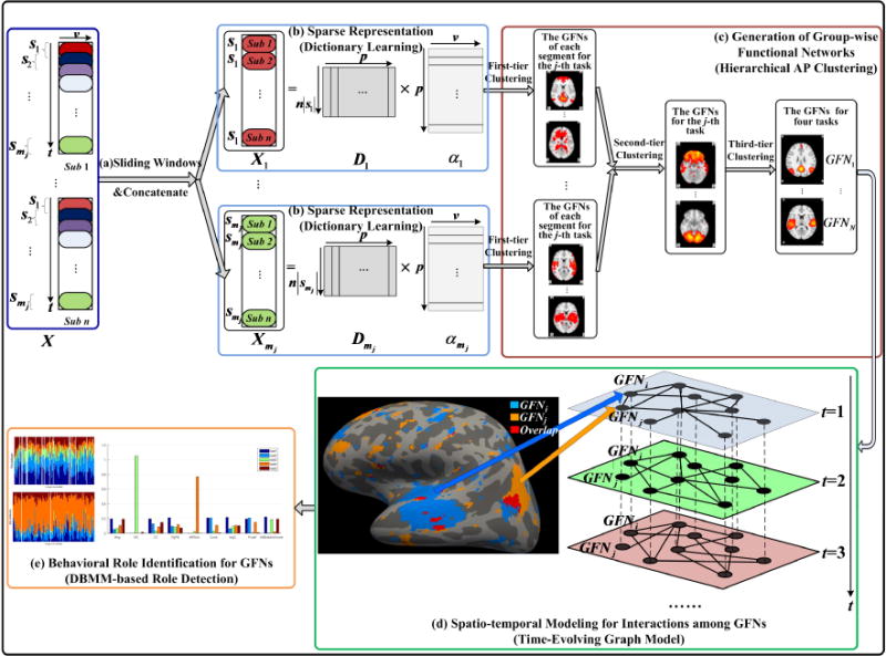
Overall computational pipeline of the proposed framework. (a) The tfMRI data of each subject are divided into multiple overlapped sliding windows and then concatenated to yield group-wise tfMRI temporal segments. (b) The group-wise temporal dynamics and the corresponding spatial maps of brain network components are obtained by the dictionary learning and sparse representation. (c) Common group-wise functional networks (GFNs) are generated by a three-tier affinity propagation (AP) clustering. (d) Spatio-temporal brain network interactions are modeled via time-evolving graphs, where the vertices and edges denote the GFNs and their spatial interactions, respectively. (e) Behavioral roles of the GFNs are identified by the effective DBMM-based role detection algorithm.

For the detailed description of the proposed methods in this paper, the following definitions and notations are used.

si(i = 1,2,⋯mj)	The i-th sliding window.
|si|	The size of si.
Xi(i = 1, 2,⋯mj)	Concatenated input matrix for si.
Di = [d1, d2⋯dP], (i = 1, 2,⋯mj)	Dictionary.
dq(q = 1,2, ⋯ p)	Atom in the dictionary.
αi(i = 1, 2,⋯mj)	Coefficient matrix.
GFNj	The j-th group-wise functional network.
FNCk,p	The p-th functional network component occurring in sk.
TEG = (V, F)	Time-evolving graph with vertex set V and edge set E.
$e_k^{ij}$	Edge between the vertices GFNi and GFNj in the k-th layer of TEG.
$w_k^{ij}$	Weight of the edge $e_k^{ij}$.
Fk ∈ ℝN×f (k = 1, 2, ⋯ M)	Feature matrix of the k-th layer of TEG.
Gk ∈ ℝN×r (k = 1, 2, ⋯ M)	Role membership matrix.
H ∈ ℝr×f	Projection matrix from the role space to the feature space.
Qk ∈ ℝN×I	Measure matrix.
E ∈ ℝr×I	Contribution matrix of the measure index to the roles.
$N_i=\{GN{F}_j|e_k^{ij}\in E\}$	Neighbor vertices of GNFi.
${\overline{N}}_i=V\backslash \left(\left\{GN{F}_i\right\}\cup N_i\right)$	Vertex set that does not contain GNFi and Ni.
‖·‖1	l-1 norm.
‖·‖F	F norm.

2.2. Data Acquisition and Pre-processing

In this paper, we use the publicly released high quality tfMRI data in Human Connectome Project (HCP) (Q1release) to develop and evaluate the proposed pipeline. Four task-based fMRI datasets including motor, working memory, language and social tfMR data collected from 68 subjects are adopted as the test bed for method development and evaluation. The main acquisition parameters of tfMRI data are as follows: 90×104×72 dimension, 220mm FOV, 72 slices, TR=0.72s, TE=33.1ms, flip angle = 52°, BW=2290 Hz/Px, in-plane FOV = 208×180 mm, 2.0mm isotropic voxels. The total time points of the four tasks are 284, 405, 316 and 274, respectively. The tfMRI data preprocessing is performed using the FSL tools including motion correction, spatial smoothing, temporal pre-whitening, slice time correction and global drift removal (Barch et al., 2013; Smith et al., 2013).

2.3. Concatenated Sparse Representation of tfMRI Data

As shown in Fig.1, in order to accurately capture the dynamic characteristics of brain activities, we firstly use a sliding time window to segment the input time series (of dimension t × v, where t is the number of timepoints and v is the number of voxels) of each subject in the j-th (j = 1, 2, 3, 4) task into m_j number of overlapping temporal segments $\{s_1,s_2,\cdots s_{m_j}\}$, with the window length of W. In this work, the overlapping segment between two consecutive windows contains 4W/5 time points, while the overlapping length can be changed. Then, the tfMRI data from the i-th window s_i(i = 1, 2, ⋯ m_j) of the j-th task across all subjects are concatenated to yield a group-wise input signal matrix X_i(i = 1, 2, ⋯ m_j). The concatenated input matrix X_i is decomposed by a l-1 regularized online dictionary learning algorithm (Mairal et al., 2010) to learn a dictionary D_i and a corresponding weighting coefficient matrix α_i. Dictionary learning aims to create a sparse representation for the input signal X_i = [x₁, x₂ ⋯ x_v]. The main process of dictionary learning is to learn an over-complete, representative basis set D_i = [d₁, d₂⋯ d_P], termed as “dictionary” and composed of “atoms” d_q(q = 1,2, ⋯ p), such that each input signal vector x_j(j = 1,2, ⋯ v) could be modeled as the form of a linear combination of basis signals (atoms) in the learned dictionary, i.e., x_j ≈ D_iα_i,j or x_i ≈ D_iα_i. In brief, the problem of dictionary learning can be viewed as a matrix factorization problem, equivalently represented by a minimization problem.

$$f\left(D_i,{\alpha }_i\right)={min}_{D_i\epsilon C_i,{\alpha }_i\epsilon {\text{ℝ}}^{p\times v}}\frac{1}{2}{\Vert D_i{\alpha }_i-X_i\Vert }_F+\mathrm{\lambda }{\Vert {\alpha }_i\Vert }_1$$ (1)

$$C_i\triangleq \{D_i\epsilon {\text{ℝ}}^{n\left|s_i\right|\times p},s.t.\forall q=1,2,\cdots p,d_q^T{d}_q\le 1\}$$ (2)

The loss function f(D_i, α_i) contains the reconstruction error term ‖D_iα_i − X_i‖_F and a sparsity penalty term ‖α_i‖₁. By imposing sparsity constraint on the coefficient matrix α_i, we can obtain sparse representation of the input signal X_i. p is the pre-defined number of dictionary atoms. λ regularizes the trade-off between sparsity (measured by l-1 norm of α_i) and the reconstruction error. |s_i| is the size of the i-th temporal segment s_i and n|s_i| is the number of rows of the dictionary D_i. In this work, the online dictionary learning method (Mairal et al., 2010) is employed for solving the minimization problem in Eq.(1) with the constraint in Eq.(2). The resultant dictionary D_i and the coefficient matrix α_i characterize the underlying temporal variation patterns and the spatial maps of functional network components of X_i, respectively (Lv et al., 2015a). As a result, p number of functional network components for each window of one task and $p\times {\displaystyle {\sum }_{j=1}^4{m}_j}$ network components for all windows of the total n number of subjects across four task scans are achieved.

2.4. Generation of Group-wise Functional Networks

We cluster all the $p\times {\displaystyle {\sum }_{j=1}^4{m}_j}$ functional network components to identify representative and common group-wise consistent functional brain networks across four tasks of all subjects. In the sparse representation of whole-brain fMRI signals, each functional network component can be represented by a high dimensional (more than 200 thousands) vector. To reduce the computational cost of the entire clustering process and produce meaningful intermediate results, a hierarchical AP clustering is employed. AP clustering is based on the concept of “message passing” between data points. Unlike other clustering algorithms, AP creates clusters by sending messages between pairs of samples until convergence. A dataset is described using a small number of exemplars (cluster centers), which are identified as those most representative of other samples. The messages sent between pairs represent the suitability for one sample to be the exemplar of the other, which is updated in response to the values from other pairs. This updating is performed iteratively until convergence, at which point the final exemplars are chosen, and hence the final clustering is given. More details are referred to (Frey and Dueck, 2007). Compared with other clustering algorithms, such as k-means or k-medoids, the AP clustering (Frey and Dueck, 2007) does not require the number of clusters to be pre-specified before running it. The cluster number can be automatically generated based on the data to be clustered. In addition, the AP clustering can achieve lower clustering errors than other algorithms and its results do not depend on the initialization (Frey and Dueck, 2007).

Based on the AP, we design a hierarchical clustering algorithm that can group the $p\times {\displaystyle {\sum }_{j=1}^4{m}_j}$ network components to obtain their common GFNs. The proposed algorithm contains three tiers. In the first tier, the AP is applied to cluster the p number of network components learned from each concatenated segment in one task across all subjects to obtain GFNs of each segment. In the second tier, the resultant cluster centers of all concatenated segments for one task are pooled together and further clustered via the AP to yield GFNs of this task. In the third tier, using the resultant cluster centers of the second tier as the inputs, common group-wise functional networks {GNF₁, GNF₂, ⋯ GNF_N} across all four tasks are obtained via the AP algorithm again. In this three-tier AP clustering, the similarity between two networks (or network components) (GNF₁, GNF₂) is measured by the spatial overlap rate (SOR), i.e., the Jaccard similarity coefficient (Lv et al., 2015b). The Jaccard similarity coefficient is defined as the size of the intersection divided by the size of the union of the two sets SM₁ and SM₂.

$$J(S{M}_1,S{M}_2)=\frac{|S{M}_1\cap S{M}_2|}{|S{M}_1\cup S{M}_2|}$$ (3)

where SM₁ and SM₂ denote the spatial maps of the two networks GFN₁ and GFN₂, respectively.

Note that, the AP clustering is performed hierarchically for two reasons. First, sparse representation of tfMRI data produces $p\times {\displaystyle {\sum }_{j=1}^4{m}_j}$ functional network components. In the experiments, p = 400, m₁ = 90, m₂ = 131, m₃ = 101 and m₄ = 87. Each network component is denoted by a 205,832-dimensional vector. If we directly perform the AP clustering for these $p\times {\displaystyle {\sum }_{j=1}^4{m}_j}$ network components, the similarity matrix contains ${(p\times {\displaystyle {\sum }_{j=1}^4{m}_j})}^2\approx 2.7\times {10}^{10}$ entries, which incurs a quite huge computational cost. Thus, we decompose the entire AP clustering into three levels, which perform network-component-level, time-window-level and task-level clustering, respectively. As a result, the computational complexity can be significantly reduced. Second, the results for clustering all network components simultaneously cannot be reused, if the number of time windows increases or more tasks are considered. As a result, re-clustering for all the samples has to be performed. In contrast, in our method, the intermediate clustering results of each level of the hierarchical AP can be directly reused in the above two cases. Thus, the proposed hierarchical structure has higher reusability.

2.5. Modeling of Temporal Evolution of Spatial Interactions among Group-wise Functional Networks

It has been shown in (Lv et al., 2015a) that multiple functional networks are simultaneously distributed in different neuroanatomic areas and substantially spatially overlapping with each other, which jointly response to external stimuli. As examples, Fig.2 shows spatial overlap/interaction relationships of three GFNs. It can be observed that different networks interact with each other with a high proportion of spatial overlaps within a specific cognitive or functional task.

Fig.2.

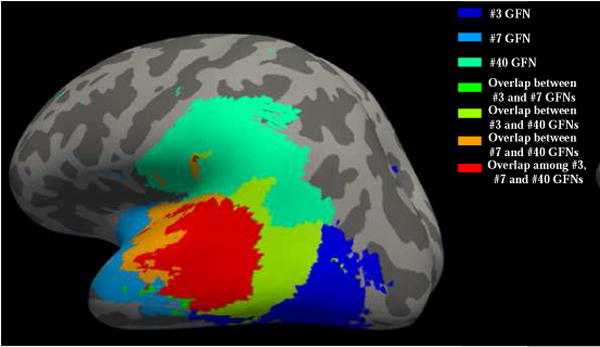
Spatial overlaps/interactions among three GFNs are plotted on the inflated cortical surface. The three networks (#3, #7 and #40) are color coded by three colors, respectively. They overlap with each other and the red area is jointly covered by all three networks. The color coding schemes are on the top right.

Furthermore, spatial interactions of the networks exhibit remarkably dynamic characterizations, which have not been examined in our prior works (Lv et al., 2015a; Lv et al., 2015b). Fig.3 gives an example, where the overlapping area between two network components corresponding to the visual network and default mode network (DMN), respectively, changes over time, although overall distributions of the spatial maps of two components are relatively stable across three time windows.

Fig.3.

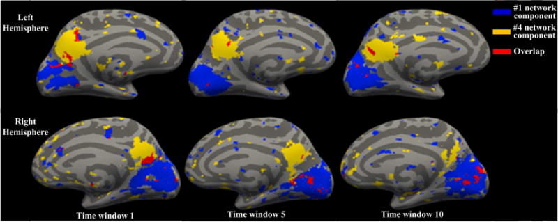
Temporal evolution of the interaction between two network components in the language task. #1 and #4 network components correspond to RSN 1 and RSN 4 (Lv et al., 2015a) and are denoted by the blue and yellow areas, respectively. The red color represents the overlapping area between the two components. Their spatial interactions present different patterns across time windows. The color coding schemes are on the top right.

To quantitatively describe the time-varying brain network dynamics, we propose a time-evolving graph based approach to model temporal evolution of spatial interactions among the obtained group-wise brain networks. The time-evolving graph, a special type of the multilayer network, is a sequence of graphs over time denoted by multiple layers, respectively. We denote the time-evolving graph by TEG = (V, E), where V is the set of vertices and E is the set of edges. Let TEG_k = (V_k, E_k) (k = 1, 2, ⋯ M) denote the k-th layer of TEG, where $V_k=\left\{v_k^i\right\}$ are the vertices in TEG_k and $E_k=\{e_k^{ij}|v_k^i,v_k^j\in V_k\}$ are the edges active in TEG_k, as shown in Fig.4. In this study, the vertex sets are the same across the different layers, i.e., V_k = V_l = V for all k and l.

Fig.4.

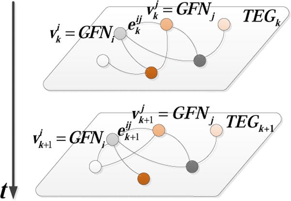
Time-evolving graph model for the representation of interaction relationships among functional networks. In each layer, the vertices denote the GFNs and the edges denote spatial overlaps/interactions between the networks. The weights of the edges measure the interaction strength between two networks.

For each task, we model temporal evolution of spatial interactions among {GFN₁, GFN₂, ⋯ GFN_N} by a undirected weighted time-evolving graph, which contains M (M = m_j for the j-th task) layers and each of them represents the interaction relationship of {GFN₁, GFN₂, ⋯ GFN_N} within the corresponding sliding time window. In each layer, the vertices represent N number of GFNs, i.e., V = {GFN_i, i = 1, 2, ⋯ N}, as shown in Fig.4. The edge $e_k^{ij}$ between two vertices GFN_i and GFN_j represents spatial interaction between them. Its weight $w_k^{ij}$ measures to what extent GFN_i and GFN_j spatially overlap in TEG_k (corresponding to the k-th sliding time window s_k). To compute $w_k^{ij}$, we first find the two functional network components (spatial maps) from the current window s_k, which have the highest similarity with the network templates GFN_i and GFN_j, respectively, and denote them by FNC_k,p and FNC_k,q. Then, we compute the normalized spatial overlap between FNC_k,p and FNC_k,q and use it as the weight $w_k^{ij}$.

$$w_k^{ij}=\frac{\left|FN{C}_{k,p}\cap FN{C}_{k,q}\right|}{v}$$ (4)

The weight $w_k^{ij}$ of the edge $e_k^{ij}$ measures to what extent spatial interaction occurs between each pair of networks at the current time window and reflects the strength of functional interaction between them.

Note that, the brain network templates (GFNs) are time independent. They are obtained by clustering all functional network components of all 68 subjects across four tasks. That is, they represent averaged and general brain activation states over time, subjects and tasks. Thus our premise is that those GFNs are not varying (as they are aggregated measurement across independent datasets), and can be used as “templates” for the nodes in TEG graphs. When computing the weight $w_k^{ij}$ of the edge $e_k^{ij}$ between two vertices GNF_i and GNF_j, spatial overlap rate of the two network components FNC_k,p and FNC_k,q, which have the highest similarity with the two templates (GNF_i and GNF_j), are used for the measurement.

Compared with other state-of-the-art graph-based brain connectivity models (e.g., Van Den Heuvel and Hulshoff Pol, 2010; Xu et al., 2016; Thompson and Fransson, 2015; Eddin et al., 2013; Marrelec et al., 2006; Cassidy et al., 2015; De Domenico et al., 2016), a notable characteristic of the proposed time-evolving graph based brain dynamic model is that it quantifies evolution of the spatial interactions among brain networks over time (layers), and thus can comprehensively describe the temporally dynamic changes of the functional interactions of brain networks.

2.6. Identifying Behavioral Roles of Functional Networks from Topology of Time-varying Spatial Interactions

From Fig.2, it can be observed that different functional networks have significantly diverse spatial overlap rates. On the other hand, as shown in Fig.3, the same connection between two specific networks changes over time. Therefore, the functional networks play different behavioral roles involved in functional brain interactions in the sense of time-varying topology of these networks. Thus, identification for behavioral role patterns of the brain networks is of particular importance for revealing the functional principles of the human brain.

To characterize and model the roles’ temporal dynamics of individual functional networks, we adopt the DBMM-based role detection algorithm (Rossi et al., 2013) to identify the behavioral roles of the vertices in the time-evolving graph. The DBMM is essentially an unsupervised learning algorithm. It is fully automatic (no user-defined parameters), data-driven (no specific functional form or parameterization) and interpretable (identifies explainable patterns), and thus it can automatically learn and discover behavioral roles of the vertices (GFNs). One of the main focuses of the DBMM is to discover different behavioral patterns of the vertices (GFNs) and model how these patterns change over time. The DBMM uses “roles” to represent behavioral patterns of the vertices. Intuitively, two vertices belong to the same role if they have similar structural behaviors in the graph. “Roles” can be viewed as sets of vertices that are more structurally similar to vertices inside the set than outside. The DBMM is a scalable, fully automatic, data-driven, interpretable and unsupervised learning approach to detecting roles from a time-evolving graph. Role identification contains two main steps, that is, feature extraction and role discovery.

In the feature extraction step, we describe each vertex as a feature vector. Any set of structural features deemed important can be used. In this paper, we choose three types of features, i.e., degree (refers to weighted degree, which is the weighted variant of the degree and defined as the sum of all neighboring edge weights (Rubinov et al, 2010)), egonet measures (Rossi et. al, 2013) and betweenness centrality (Freeman, 1977). Degree is one of the most essential structural features of a vertex within graphs. The egonet of a vertex is a subgraph that consists of this vertex (ego) and the vertices to whom the ego is directly connected to plus the edges among them. The egonet serves as a local feature of the graph to measure local connectivity of each vertex. Betweenness is a centrality measure of a vertex within a graph, which quantifies the number of times a vertex acts as a bridge along the shortest path between two other vertices. It serves as a global feature to measure centrality of a vertex. In our functional brain interaction model, the betweenness centrality can capture the influence that one functional network has over the flow of information between all other functional networks. Then, we aggregate the three types of features using the mean of each vertex and its neighbors and create recursive features, until no new features can be produced. After each aggregation step, similar features are pruned using logarithmic binning. The resultant features are denoted by F_k ∈ ℝ^N×f (k = 1, 2, ⋯ M).

Note that, although a certain degree of correlation exists among the structural features used in graph theory, the step of feature pruning ensures that redundant or closely correlated features are removed. In the paper, degree, egonet, betweenness are selected to initialize the recursive process of feature generation for two main considerations. First, they are the most representative features in graph theory. The combination of them can provide initial topology characterization for vertices’ behaviors and fully represent various properties of structural features of graphs. Second, as emphasized in (Henderson et al., 2011), any real-valued feature can be used to generate recursive features without restricting to a particular one. But on the other hand, we do not hope that too many artificial features are involved in the process of recursive feature generation and updating, as it may weaken the ability to discover latent roles from graph topology.

In the role discovery step, behavioral roles of the functional networks are automatically uncovered using the extracted features. For the concatenated feature matrix $F={[F_1^T,F_2^T\cdots F_M^T]}^T$, where F_k ∈ ℝ^N×f (k = 1, 2, ⋯ M), a rank-r approximation is computed by minimizing Eq.(5) with nonnegative matrix factorization (NMF).

$$f\left(G,H\right)=\frac{1}{2}{\Vert F-GH\Vert }_F^2$$ (5)

where $G={[G_1^T,G_2^T,\cdots G_M^T]}^T$, G_k ∈ ℝ^N×r(k = 1, 2, ⋯ M) is non-negative and denotes the role membership matrix, of which each row represents a vertex’s membership in each role, H ∈ ℝ^r×f is a non-negative projection matrix from the role space to the feature space. Note that, H acts on the whole feature matrix F of the entire TEG, rather than individual layers. Each column of H represents contributions of the membership of a specific role to the features. The set of role membership matrices {G_k (k = 1, 2, ⋯ M)} provides distributions of the role membership across all layers. The role number r is determined by the minimum description length criterion (Rissanen, 1978).

It is worth pointing out that the identified roles are obtained from an unified framework of the TEG in the statistical sense. They are the outcomes considering the entire interaction process of all vertices across all layers of the TEG simultaneously, rather than the interactions in individual layers, which makes it possible to characterize and analyze the unified behavioral role dynamics of the functional networks over time.

The DBMM cannot directly present specific interpretations on the meaning of each role, although r number of roles are automatically generated. To quantitatively interpret the resultant roles with respect to well-known vertex’s indices in graph theory, such as degree, egodegree, betweenness, clustering coefficient, PageRank, effective size, constraint, eigenvector centrality, participation coefficient and within-module degree, a measure matrix $Q={[Q_1^T,Q_2^T,\cdots Q_M^T]}^T$ is constructed by aggregating these indices of each vertex in each layer together, where Q_k ∈ ℝ^N×I(k = 1, 2, ⋯ M), I denotes the number of the indices. Then, given G and Q, a non-negative matrix E ∈ ℝ^r×I is computed by the NMF such that GE ≈ Q. The i-th column of E interprets contributions of all roles to the i-th index. For instance, assume that the i-th measure index is betweenness, if the entry in the j-th row and i-th column of E is largest in the i-th column, i.e., the j-th role has the highest betweenness centrality, then we attempt to interpret the j-th role as a bridge between different vertices in the graph.

Actually, each role has multiple potential interpretations, which depends on the selected indices. The index with the highest contribution to a role gives the best interpretation of this role and reveals its major function in dynamic spatial interactions among functional brain networks. Note that, role interpretation has no any impact on the results of role identification. It only provides a potential meaning for each identified role.

3. Results and Discussions

3.1. Generation of Group-wise Functional Networks

To infer functional networks (Section 2.3), the dictionary size p is set as 400 and the sparsity level λ is set to 2.1 according to our prior experiences (Lv et al., 2015a). Our extensive observations show that as long as the sparsity level is within a reasonable range (in this study, from 1.8~2.5), the sparse representation results are largely the same. The length of the sliding window is W = 15. In this paper, we assume that transitions of brain states mainly result from alternations of external blocked task stimuli. To this end, we examine the duration of each block of task stimulus signals. For an instance, the duration of a single block in motor task spreads from 5TRs to 17TRs, while the other three tasks have somewhat longer block durations (the maximum durations of a single block in working memory, social and language tasks are 32TRs, 57TRs, and 39TRs, respectively). Based on these observations, we take 15TRs as the window length. Firstly, it can capture the abrupt transitions among brain states induced by the task stimulus signals. Secondly, it is reasonably long to prevent authentic fluctuations blinded by noises. Especially, the proposed GFN generation and role discovery are based on group-wise analysis, which is less sensitive to noises when taking a relatively small window length. In the experiments, we tried different window lengths (e.g., 30TRs on motor tfMRI data) and the results do not change significantly.

After learning the group-wise network components by the concatenated sparse coding, we use the proposed three-tier AP algorithm to cluster these components into functional networks (Section 2.4). As a result, 54 GFNs are obtained, i.e., N = 54, which is automatically determined by the AP algorithm. Fig.5 shows several examples of the obtained GFNs, which are in consistency with the ten well-defined RSNs in the literature (Smith et al., 2009). The rest of 44 GFNs are shown in Supplemental Fig.1. The results in Fig.5 suggest that the group-wise concatenated sparse representation and the proposed hierarchical AP clustering algorithm can achieve meaningful and high-quality functional networks.

Fig.5.

The generated GFNs and templates of the 10 well-studied RSNs.

3.2 Comparisons between Spatial and Temporal Patterns of GFNs and Their Interactions

In the paper, we use a time-evolving graph to model the temporal evolution processes of spatial overlaps among brain networks. It is a natural way to represent dynamic variations of states of the brain networks. The key points of this model are the spatial patterns of brain networks and their spatial interactions. To clarify the rationality of the choice for describing interactions among GFNs with spatial patterns, we perform two experiments. First, we examine correlations between the spatial activation areas of the 54 GFNs and the task contrast designs, and compare them with correlations between the temporal variations of the dictionary atoms and the task contrast designs. Specifically, for each task, we compute the activation areas of the 54 network components in each layer of the time-evolving graph. As stated in Section 2.5, the time-evolving graph contains M layers. Thus, each spatial brain network forms a M-dimentional activation area vector in each task. We calculate the Pearson correlation coefficient (PCC) between this vector and the task contrast designs, and then obtain the mean and standard deviation of the absolute value of PCCs over the 54 networks, as shown in Supplemental Tables 1–4. As for the temporal variation patterns of the network components, we also compute the correlation relationships between the corresponding dictionary atoms and the task contrast designs in the same way, and the results are also shown in Supplemental Tables 1–4. From this comparison, we find that the spatial variations of the brain networks exhibit distinctly closer correlations with all the task designs than the temporal variations in the motor, working memory and language tasks, while in the social task, two variations have similar correlations. Thus, the spatial patterns of the functional networks exhibit more consistent dynamic behaviors and variation rules with the task stimuli.

To further investigate the effectiveness of the proposed time-evolving graph model for characterization of spatial interaction patterns among functional networks, we compare the correlations between spatial interactions and task contrasts with those between temporal interactions and task contrasts. Specifically, for the spatial interactions, the weight of the edge between any pair of GFNs is computed by Eq.(4). The degree of each GFN is the sum of all neighboring edge weights. In contrast, the weight for the temporal interaction between two GFNs is obtained by computing the PCC between their corresponding dictionary atoms (Lv et al., 2016; Zhao et al., 2016), and the degree is computed in the same way as the spatial interactions. Then, for each task, we compute the degree of the 54 GFNs in each layer respectively for spatial and temporal interactions. As a result, each GFN has two degree vectors with M dimension. Then, the PCCs between the two degree vectors and the task contrasts are computed, respectively. The mean and standard deviation of the absolute value of the PCCs over the 54 GFNs are given in Supplemental Tables 5–8. It can be seen that spatial interactions present larger correlations and consistency with the task contrasts than temporal interactions. Therefore, utilization of spatial patterns and their interactions to model dynamics of brain networks is more reasonable and effective.

3.3. Modeling and Role Discovery of Dynamic Spatial Interactions among GFNs

Temporal evolutions of spatial interactions among the identified 54 GFNs in each task are represented by a time-evolving graph (Section 2.5). The total time points of the motor, working memory, language and social tasks are 284, 405, 316 and 274, respectively. The time window length is W = 15 and the overlapping segment between two consecutive windows contains 4W/5 = 12 time points, i.e., the sliding step size is 3. As a result, the layer numbers, i.e., numbers of the time windows, of the four graphs are M_m = 90, M_w = 131, M_l = 101 and M_s = 87, respectively.

To focus on more meaningful interactions and reduce the influence of noises, 20% edges with low weights are removed from each layer. Then, the DBMM algorithm is applied on the time-evolving graph of each task to examine the roles’ temporal distributions and behavior patterns of each vertex. The role number is automatically decided by the minimum description length criterion. Eventually, all four tasks consistently have five roles (more details in the following paragraphs). Supplemental Fig.2 shows the role mixed-memberships of the 54 vertices (each vertex representing a GFN) in four tasks, respectively, where almost all functional networks simultaneously exhibit five roles during dynamic spatial interactions with other networks. Nevertheless, these five roles have different contributions among behavioral patterns of the networks in terms of role memberships. The major role of a network is considered as the one with the largest membership. Fig.6 gives the quantitative role interpretations for the five roles, where the measure indices contain degree, egodegree, betweenness centrality, clustering coefficient, PageRank, effective size, constraint, eigenvector centrality, participation coefficient, as well as within-module degree. Their definitions and interpretations are listed in Supplemental Table 9, where the clusters (or communities) involved in the computation of the participation coefficient and the within-module degree are created by the community detection algorithm (Blondel et al., 2008). In order to offer specific interpretations for five roles, we calculate the contributions E of the measure indices to the roles by solving GE ≈ Q via the NMF. The average contributions over time windows are presented in Fig.6.

Fig.6.

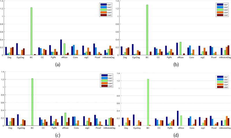
Role interpretations of the vertices in four tasks. The horizontal axis represents various indices in graph theory and the vertical axis represents characteristics of five roles corresponding to individual indices. (a) Motor task. (b) Working memory task. (c) Language task. (d) Social task.

We can find from Fig.6 that the five behavioral roles have almost common interpretations across four tasks. The role 1 represents that the vertex has the highest degree, egodegree, clustering coefficient, PageRank, eigenvector centrality and participation coefficient. This behavior pattern is straightforward to interpret, which characterizes the centrality of the graph, i.e., the most influential vertex within the graph. In other words, if a vertex mainly takes on the role 1, it should be the centrality of the graph. For the role 2, it has the highest constraint degree. When a vertex GFN_i mainly takes on the role 2, it largely depends on its neighbor vertices that are linked to GFN_i by edges and denoted by $N_i=\{GF{N}_j|e_k^{ij}\in E$. The connection relationship between the vertex GFN_i and the vertices in ${\overline{N}}_i=V\backslash \left(\left\{GF{N}_i\right\}\cup N_i\right)$ (i.e., the vertex set that does not contain GFN_i and its neighbor vertices N_i) mainly depends on N_i. If we remove the edges between the vertex GFN_i and some vertices in N_i, the connectivity between GFN_i and the vertices in ${\overline{N}}_i$ will be significantly reduced, while the connectivity between N_i and ${\overline{N}}_i$ can be hardly affected. In addition, the vertex in the role 2 has a relatively high participation coefficient. Thus, it seems that the vertex is locally connected with different clusters to a certain extent. As for the role 3, it has the highest betweenness centrality, which indicates that the vertex taking on the role 3 could be the bridge between the other vertices. Moreover, the effective size of such a vertex is relatively high, meaning that the subgraph composed of this vertex and its neighbors has little redundancy and information transfer within the subgraph largely depends on this vertex. Therefore, the vertex is likely to play a role of the center of a star subgraph.

For instance, the major role of the vertex #1 in the social task is the role 3 during most of the time. Likewise, the vertices #50 and #42 present a similar characteristic with the vertex #1, since the role 3 accounts for a high ratio in their memberships. We further examine the topological structure of the vertices #1, #42 and #50, as shown in Fig.7. In Fig.7(a), the vertex set N_1,42 = {#20, #26, #36, #41, #48, #54} contains the neighbors with relatively high weights (larger than 2.0e⁻³) of the vertices #1 and #42. It can be observed that both vertices #1 and #42 constitute the centers of this subgraph. The edges that connect these two vertices with their neighbors have significantly higher weights, while the vertices in N_1,42 interconnect with each other by the edges with lower weights. Likewise, in Fig.7(b), the vertex #50 is the center of the subgraph composed of itself and its neighbor vertices N₅₀ = {#4, #8, #9, #17, #25, #30, #35}. The roles 4 and 5 represent vertices with high within-module degree as well as low participation coefficient and effective size, which implies that they are active within a local cluster but do not act as connectors between clusters. If a vertex mainly takes on the role 4 or the role 5, it builds strong connections with the other vertices in the same cluster, while it has weak connections with the vertices in other clusters. This type of vertices has an important influence within a cluster, whereas they cannot serve as the global centrality of the whole graph, e.g., the vertex #1 (RSN 1) in the motor and the language tasks, as well as the vertex #2 (RSN 2) in the motor task.

Fig.7.

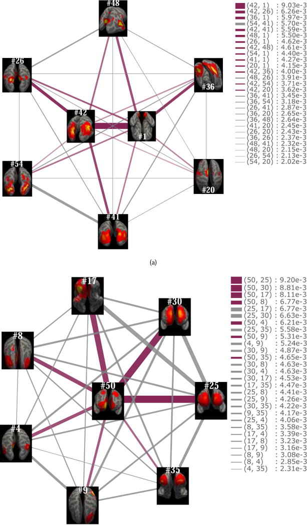
Star subgraphs. The subgraphs contain one or two center vertices. The edges connecting the center with its neighbors have higher weights than the edges between the neighbor vertices of the center. (a) Both the vertex #1 and the vertex #42 serve as the centers of the subgraph composed of themselves and their six neighbors. (b) The vertex #50 is the center of the subgraph composed of itself and its seven neighbors.

3.4. Analysis and Comparison of Behavioral Role Patterns of Functional Networks

We examine the major roles of each GFN across four tasks. Among the #1~#10 GFNs (10 RSNs), the #1 GFN distinctly takes on the role 4 in the motor and language tasks. The #2 GFN has high degree, within module degree in the language task, and hence serves as a local centrality or hub in a cluster. The #3 GFN mainly takes on both the role 2 and the role 1 in all four tasks. The #4, #5 and #6 GFNs take on the hybrid roles. They comprise at least three memberships that account for relatively high proportions. Note that, the #6 GFN is activated more frequently in the motor task than in the other three ones. Especially, the #6 GFN rarely occurs in the language task. Ratios of the role memberships 1, 3, 4 and 5 of the #6 GFN are approximately equal in the motor task. The #7 GFN distinctly takes on the centrality role in the motor, working memory and social tasks. The averaged ratios of the first membership are 39.7%, 47.9% and 44.3%, respectively. The #8 and #9 GFNs mainly act as the centrality in the working memory task. Their averaged ratios of the first membership are 48.4% and 45.0%, respectively. Like the #3 GFN, the #10 GFN mainly takes on the roles 2 and 1 in four tasks.

We also notice that the #7 GFN (RSN 7) maintains almost consistent behavioral pattern dominated by the role 2 over time in the language task, while it mainly takes on the role 1 (centrality of the graph) in the other three tasks. We visualize in Fig.8(a) the mean activated area of the #7 GFN, which is obtained by computing the averaged spatial map of its network components over all the time windows. We find that in the motor, working memory and social tasks, the mean activation areas of the #7 GFN cover 9447, 8972 and 8364 volume voxels, respectively, whereas only 7089 voxels are activated in the language task. Moreover, the mean ratios of the activation area of the #7 GFN to sum of the activation areas of all 54 GFNs are 1.76%, 1.77%, 1.70% and 1.49% in motor, working memory, social and language tasks, respectively. Likewise, the mean ratios of the degree of the #7 GFN are 1.83%, 1.83%, 1.75% and 1.31%, respectively. To evaluate the activation areas and their ratios of the GFN #7 in four tasks in a statistical sense, we perform a set of hypothesis tests. The results are shown in Supplemental Tables 10–11 and Figs. 3–4. From these experiments, we can find that the GFN #7 presents a significantly smaller activation area and its ratio in the language task than in other three tasks. We further check the overlapping activation area of the #7 GFN of the four tasks, as shown in Fig.8(b). There are 3800 volume voxels in total activated in all four tasks and 1628 voxels exclusively activated in the language task. This reveals that the #7 GFN has a distinct activation pattern in the language task. In addition, the less activation area, ratio of activation area and ratio of degree of the #7 GFN lead to weaker spatial interactions with the other networks. As a result, the #7 GFN does not take on the centrality role in the language task, although it is fairly active.

Fig.8.

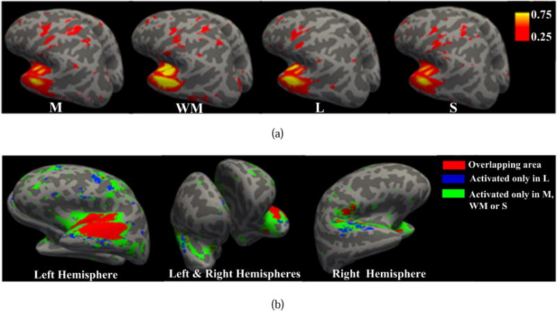
Activation areas of the #7 GFN. (a) Different activation areas of #7 GFN in four tasks. Compared with the other three tasks, the language task has a smaller activation area. (b) The red color denotes the overlapping area of the #7 GFN among all four tasks. The blue and green denote the activation area only in the language task and that only in the other three tasks, respectively.

Except 10 RSNs, there are some other GFNs that serve as the centrality of the time-evolving functional interaction graph, for instances, the #11 and #51 GFNs in all four task, as well as the #12 GFN in the working memory tasks. After further examining the time-evolving role mixed-memberships of each vertex, we find some distinct structural behavior patterns represented by these vertices. a) Several vertices have almost homogeneous behavioral patterns. In other words, the vertices for the most part take on a single role, e.g., the #24 vertex consistently takes on the role 2 over time in both motor and working memory tasks, and the #28 vertex also takes on the role 2 in both working memory and language tasks. b) Some vertices’ behavioral patterns are relatively stable over time, e.g., the #4 and #8 vertices in the motor task, the #51 and #53 vertices in the language task. c) Some vertices’ role behaviors change frequently over time, which exhibit strong functional diversity and heterogeneity, e.g., the #1, #2 and #54 vertices in the working memory task, as well as the #46 vertex in the motor task.

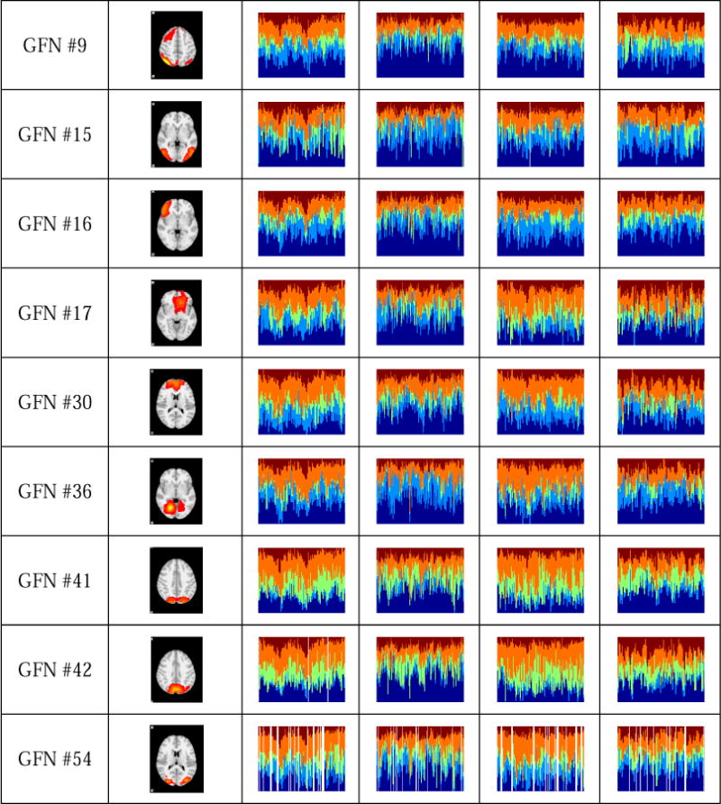
A team of five experts quantitatively and qualitatively examined differences of time-evolving role mixed-memberships of each vertex across four tasks by both visual inspection and computation of similarity between mixed-memberships. They checked the mixed-memberships separately, and the final results are based on the agreement reached by a voting procedure. Finally, 14 brain networks, including the #1, #4, #6, #7, #8, #9, #15, #16, #17, #30, #36, #41, #42 and #54 GFNs, exhibit remarkably different behavioral patterns across four tasks, while the other 40 GFNs have similar role distributions across four tasks. The spatial maps and role mix-memberships of these 14 GFNs are given in Fig.9. Among them, #1, #4, #6, #7, #8 and #9 are from the standard RSNs. The #1 GFN is the medial visual area. It mainly takes on the role 4 in the motor and language tasks, and hence serves as an active vertex in a local cluster (or community). In the working memory task, the #1 GFN takes on role 1 and role 4 alternately. In the social task, the #1 GFN tends to play a role of the bridge between other GFNs, since roles 1, 3, 4 and 5 account for approximately equal proportions, as discussed in Sections 3.2 and 3.3. The #4 GFN is the DMN. It has relatively stable distributions on five role memberships. Specifically, the #4 GFN has high within-module degree, betweenness and constraint degree in the motor task. It is worthwhile to note that, the #4 GFN has large role membership 1 and approximately equal memberships of the other four roles in the working memory task, thus it may serve as a hub vertex in this task. The #6 GFN is the sensorimotor area. It is a motor-related network, which occurs more frequently in the motor task, as shown in Supplemental Fig. 2. The #7 GFN corresponds to the auditory area. As discussed earlier, this network mainly acts as the centrality in the motor, working memory and social tasks, while it takes on the role 2 in the language task. The #8 GFN is the executive control area. It serves as the centrality almost all the time in the working memory task. In the other three tasks, the #8 GFN has high role memberships 1, 3 and 4, and they are stable over time. Thus, this network is more likely to act as a hub vertex. As for the #9 GFN, it is the frontoparietal area. Comparing the ratio of the role membership 1 in the working memory task with that in the other tasks, we find that the #9 GFN tends more clearly to serve as the centrality in the working memory task. Likewise, the #30 GFN also behaves more actively in the working memory task than in the other three tasks. For the #15 GFN, it has a larger membership of the role 3 and a smaller one of the role 2 in the motor task. The #17 GFN has a larger membership of the role 4 in the language task than in the other three tasks. The #16 GFN has a larger role membership 2 in the language task than in the other three ones. The #36 GFN has a similar behavioral pattern (role 4) in the motor and language tasks, where it is more active within a cluster, but it more tends to involve in different clusters in the other two tasks. The #41 and #42 GFNs present similar role patterns. They have high role membership 4, and hence they are more locally active in the motor and language tasks. In contrast, their role memberships 1 and 3 are large in the working memory and social tasks, thus they have a greater global influence in these two tasks. The #54 GFN mainly takes on role 4 in both the motor and the language tasks and hybrid roles in the other two tasks, respectively.

Fig.9.

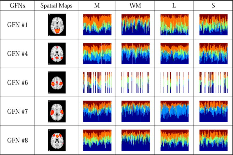
Fourteen GFNs which exhibit different behavioral patterns across four tasks. Each row presents time-evolving role mixed-memberships of four studied tasks of a GFN. The horizontal axis represents the time window (the layer of the time-evolving graph), while the vertical axis represents the role distribution in each time window. Five colors represent five different roles learned from the time-evolving graph model. The inactivity is represented by the white bars. According to interpretations on the roles in Fig.6, the role 1 represents the centrality of the time-evolving graph, which implies that the vertex in role 1 is the most influential in the graph. In contrast to the role 1, the role 2 represents that the vertex plays a less important role. The role 3 represents the bridge between other vertices of the graph. The roles 4 and 5 represent that the vertex has an important influence within a cluster, whereas it cannot serve as the global centrality of the whole graph.

We also notice that some functional networks exhibit similar role patterns in all the four tasks. For instance, the #1, #41 and #42 GFNs, as well as the #24 and #28 GFNs. Their spatial maps and time-evolving role mixed-memberships are shown in Fig.10.

Fig.10.

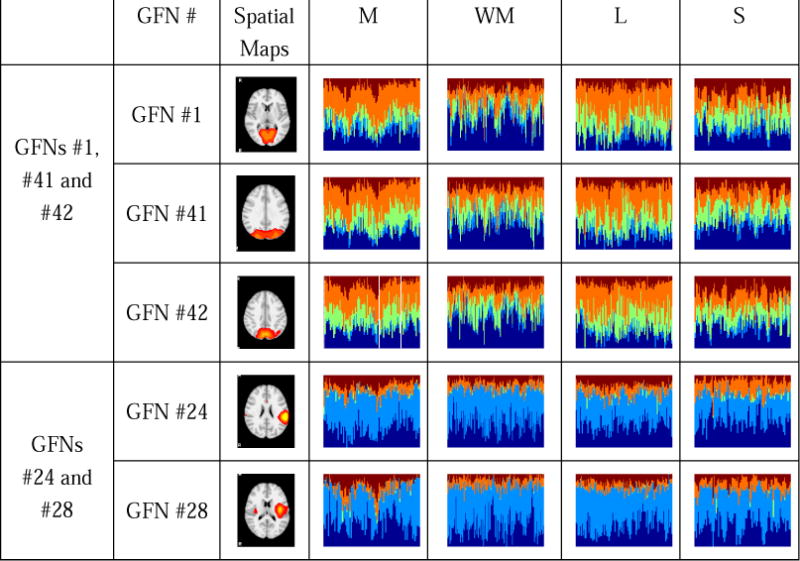
GFNs which exhibit similar role patterns for all the four tasks, where the GFNs #1, #41 and #42 present obviously similar mixed-memberships distributions, and so do GFNs #24 and #28.

3.5. Role Dynamics of Functional Networks

As shown in Supplemental Fig.2., the behavioral roles of the networks exhibit remarkable temporal variations. Here, we investigate temporal dynamics of the roles and how likely the complex role dynamics stems from external task stimulus. To this end, we focus on the relationship between the role mixed-membership dynamics and the task contrast designs. By examining their temporal correlation, we find that the behavioral roles of the brain networks tend to follow task paradigm curves. In addition, different task contrast designs impose distinct influences on temporal change of the roles. Fig. 11 gives the temporal response curves of the #13 and #8 GFNs to the contrast designs in the language task. In Fig.11(a), the role 1 and the role 2 of the #13 GFN present opposite temporal variation patterns. The role 2 varies with the task paradigm curve of contrast 1, whereas the role 1 is negatively correlated with the contrast 1. Likewise, for the contrast 2 in Fig. 11(b), the two roles also exhibit different correlations with the task design. In Fig. 11(c) and Fig.11(d), the #8 GFN has opposite temporal dynamics between the role 1 and role 2. By further comparing Fig.11(a) and Fig. 11(c), the role 1’ temporal dynamics of the #13 GFN is obviously opposite to that of the #8 GFN.

Fig.11.

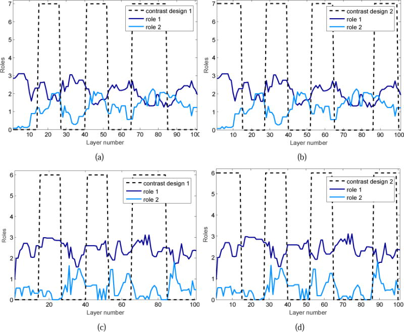
Temporal response curves of the two roles of the #13 and #8 GFNs to the contrast designs in the language task. (a) Variation of the #13 GFN’s role 2 is evoked by the task contrast 1. The Pearson correlation coefficient (PCC) between the response curve of the role 2 and the paradigm of the contrast 1 is PCC=0.49, which implies that the role 2 of this network follows the task design closely. (b) The #13 GFN’s role 1 synchronously varies with the task contrast 2. The Pearson correlation coefficient between them is PCC=0.56. (c) Variation of the #8 GFN’s role 1 follows the task contrast 1. The Pearson correlation coefficient between them is PCC=0.55. (d) Response curve of the #8 GFN’s role 2 is induced by the contrast design 2. The Pearson correlation coefficient between them is PCC=0.46.

We examine the role dynamics of the 10 RSNs. Many RSNs present roles’ temporal variations induced by the task designs and different RSNs have diverse role patterns with respect to the task designs. Among the 10 RSNs, the #4 and #9 RSNs present notably temporal correlation with the task paradigms in all the four task. Fig.12 shows some temporal variations of the major roles of the #4 and #9 RSNs, wherein the PCC between the role variations and the task designs are given. It can be seen that the major roles of these two RSNs are closely correlated with the corresponding task designs. They are either excited or inhibited by the task stimuli. Except the RSNs, some task-related networks (Lv et al., 2015a) are strongly correlated with the task contrasts. Some of their roles’ temporal variations are shown in Supplemental Fig. 5.

Fig.12.

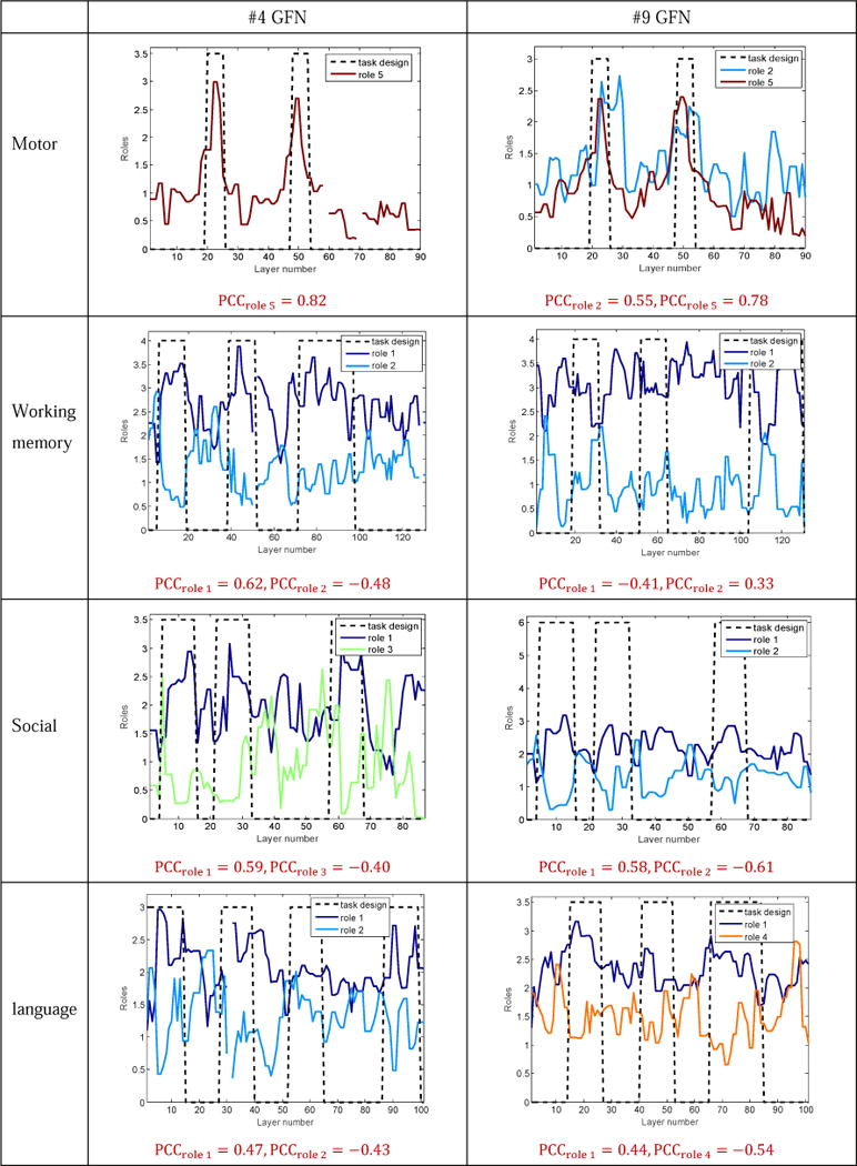
Role dynamics of the #4 and #9 RSNs in all four tasks. Major roles of the #4 and #9 RSNs can follow the task paradigm curves. Roles of these two RSNs present either positive correlations or negative correlations with the contrast designs.

In addition, in the motor task, the role 5 of almost all the GFNs has a similar response profile, which is induced by the task contrast 6 (tongue). Supplemental Fig. 6 shows the entire response curves of the five roles and the degree of the 10 RSNs to the contrast 6 of the motor task. We also find that the other four roles are affected by the contrast 6 to a large extent. They are either evoked or suppressed by this contrast. Furthermore, the degree of the 10 RSNs increases when the tongue task is implemented, especially for the #1, #3, #6 and #9 RSNs.

It can be observed from the role mixed-memberships of the 54 GFNs in Supplemental Fig.2 and the role dynamics of the GFNs in Figs.11–12 that the GFNs exhibit evidently dynamic role fluctuations during their spatio-temporal interaction process. To examine the likelihood these fluctuations are neuronally relevant, rather than attributed to some exquisitely simple statistical process, we adopt the Fourier phase-randomization to generate surrogate of the original motor tfMRI data, and then carry out the remainder of the proposed pipeline on the surrogate data. This experiment is run five times to get better estimates of the statistics under interest. We compare the two groups of results obtained using and without using the phase-randomization from two aspects. First, we examine the differences between the 54 GFNs’ activation areas computed by the original data and the surrogate data, respectively. Specifically, for each GFN, its activation areas in M layers of the time-evolving graph model constitute a M-dimensional vector. Then, we concatenate this vector of the 54 GFNs into a 54 × M-dimensional activation area vector. We use the Kolmogorov-Smirnov statistic to measure the difference between the two activation area vectors corresponding to the original and surrogate data, respectively. The results of five runs are given in Supplemental Table 12. It can be seen that activation areas of the 54 GFNs present significant difference between the original and surrogate data. Second, we examine the differences between two groups of role mixed-memberships of the 54 GFNs. We start with visual inspection to compare two groups of results and find obvious differences occur between them. To make a further quantitative comparison, Kolmogorov-Smirnov test is also adopted. Specifically, we concatenate the five rows of the role mixed-membership matrix of each GFN together to obtain a r × M-dimensional vector. Then, the Kolmogorov-Smirnov test is employed for each GFN to quantify the difference between its two role mixed-memberships corresponding to the original data and the surrogate data. The results shown in Supplemental Table 13 imply that the role mixed-memberships of most GFNs extracted from the original tfMRI data are significantly different from those extracted from the surrogate data.

Likewise, the role dynamics induced by the task designs exhibits large differences between the results obtained from the original and surrogate data. Supplemental Fig.7 shows an example, where the roles 1 and 5 of the #5 GFN computed by the original tfMRI data have a strong correlation with the task design, while they are nearly uncorrelated with the task design in the result obtained by the surrogate data.

Comparisons between results of the original and surrogate data demonstrate that the observed variations of activation areas and fluctuations of the role mixed-memberships of the GFNs from the original fMRI data couldn’t come from merely random fluctuations and are more likely to represent dynamic neuronal connectivity changes.

3.6. Dynamic Overlaps among Functional Networks

As discussed in (Lv et al., 2015a), highly heterogeneous regions reveal the functional interaction patterns of the brain networks. Here, we examine highly heterogeneous regions and their dynamic attributes over different sliding time windows and across different tasks. We find that many pairs of networks have dramatically dynamic interactions and overlaps, which are affected by the task designs. For instance, dynamic spatial overlaps between the #2 and #54 GFNs in the motor and working memory tasks are shown in Fig. 13. The #2 GFN is an RSN and the #54 GFN is a working memory task-related network. They have similar behavioral roles in the motor and working memory tasks. In the motor task, the Pearson correlation coefficient between the entire task contrast and the dynamic overlap of the two GFNs is 0.60. Fig. 13 (a) shows three spatial overlaps corresponding to two time points C₁ and C₂ within the task contrast 6 (tongue) and one time point I₁ within the idle period, respectively. Obviously, the overlap between these two GFNs increases significantly when the task contrast 6 occurs and decreases to the minimum value at the idle period. In contrast, in the working memory task, the task contrasts and the overlap of the #2 and #54 GFNs exhibit negative correlation. Fig. 13 (b) shows six spatial overlaps of the two GFNs at three time instants C₁, C₂ and C₃within the contrast periods and around three switch points S₁, S₂ and S₃ between two successive contrasts, respectively. The two networks present weak spatial overlaps/interactions at C₁, C₂ and C₃, while their overlaps/interactions become significantly strong at S₁, S₂ and S₃. These results show the dynamic attributes of the spatial overlaps/interactions of the brain networks and their dependence on the task design.

Fig.13.

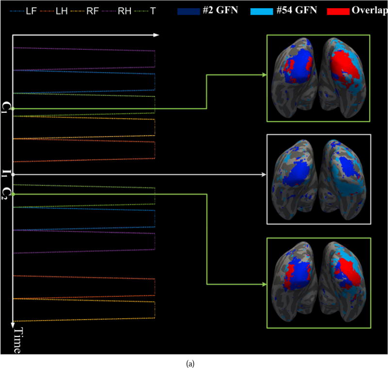
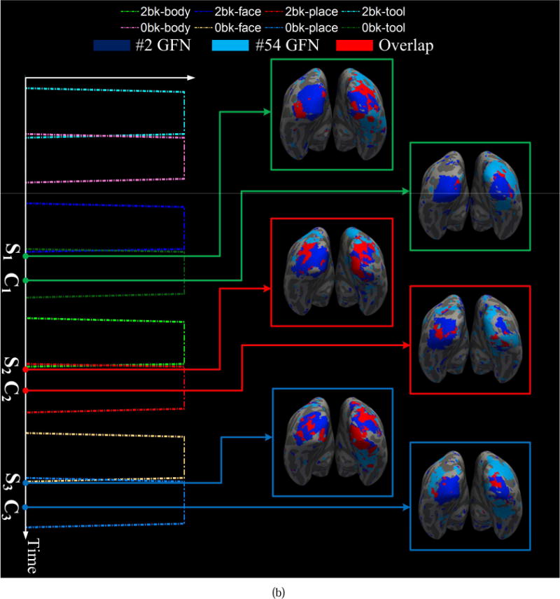
Dynamic spatial overlaps/interactions between the #2 and #5 GFNs. (a) The spatial overlap between the two GFNs varies with the task contrast in the motor task. The contrast design 6 excites the overlap area to increase dramatically at time point C₁ and C₂, while it decreases to almost zero at the idle time point I₁. (b) The spatial overlap between the two GFNs is negatively correlated with the task contrast in the working memory task. That means the contrast design of the working memory task may inhibit the functional interaction of these two networks.

We also investigated the spatial overlap/interaction relationships among three networks. Dynamic characteristics similar to the case of two networks can be found in some three-networks groups. For instance, the overlap area among the #25, #30 and #50 GFNs is positively correlated with the contrast 1 of the language task, as shown in Fig. 14. Likewise, negative correlation occurs between the spatial overlap of the #1, #41 and #42 GFNs and the contrast design in the working memory task. Fig. 15 shows correspondence of the spatial overlap among these three GFNs to the contrast design.

Fig.14.

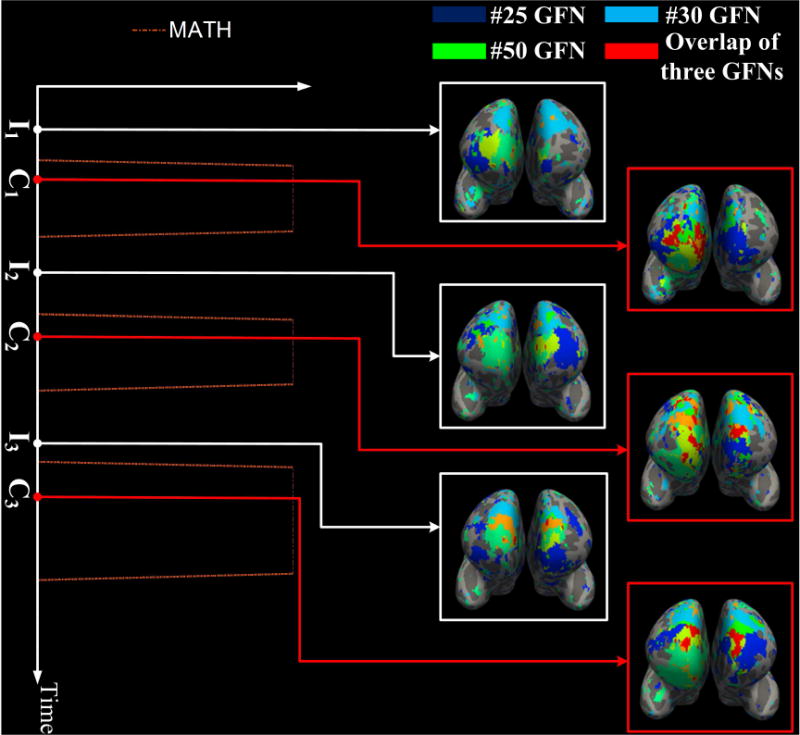
Dynamic spatial overlaps/interactions among three GFNs #25, #30 and #50. The spatial overlap among them changes with the contrast 1 of the language task. The Pearson correlation coefficient between the overlap area and the contrast 1 is PCC = 0.58. At time points C₁, C₂ and C₃ within the contrast designs, the overlap area of the three networks reaches a peak value, while at three idle time points I₁, I₂ and I₃, the spatial overlap reduces to a minimal value.

Fig.15.

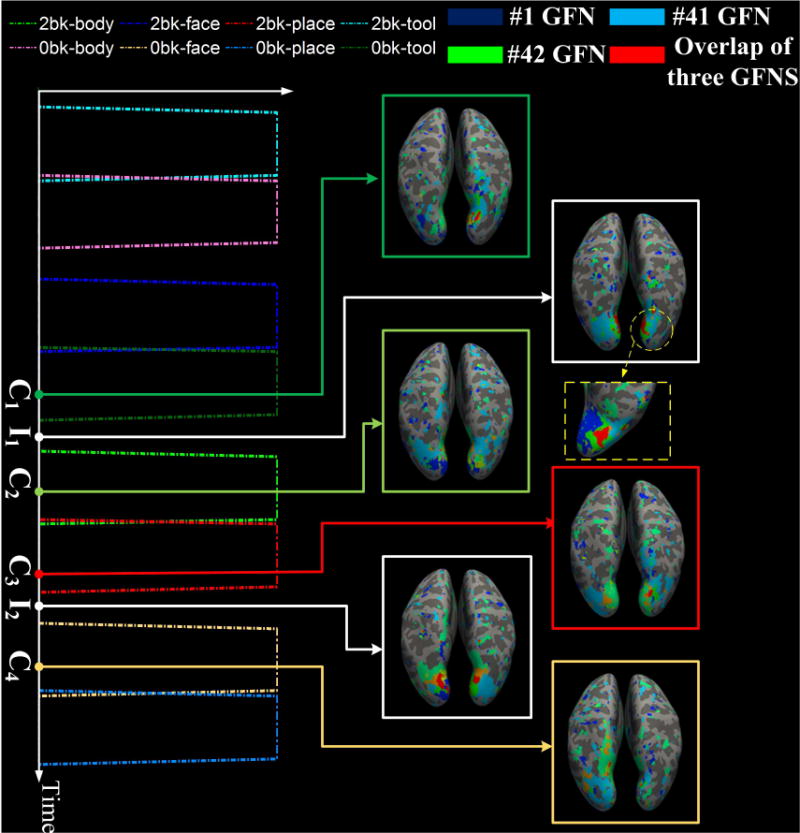
Dynamic spatial overlaps/interactions among three GFNs #1, #41 and #42. The spatial overlap among them is negatively correlated with the entire contrast design of the working memory task. The Pearson correlation coefficient is PCC = −0.43. At time points C₁, C₂, C₃ and C₄ within the contrast designs, the overlap area of three networks reduces to a minimal value, while at two idle time points I₁ and I₂, which lie between C₁ and C₂, as well as C₃ and C₄, respectively, the overlap area reaches a peak value.

3.7. Reproducibility Verification of the Proposed Methods

By using our computational pipeline, 54 group-wise functional networks are generated from all the four tasks by pooling the networks obtained from each task together to implement the third-tier AP clustering. We denote the set consisting of these 54 networks by GFN_MWLS.

In this experiment for reproducibility verification, we only considered the motor and working memory tasks and re-performed the third-tier AP clustering on their individual networks. As a consequence, 45 group-wise common functional networks were obtained. They constitute the network set GFN_MW. By comparing GFN_MW with GFN_MWLS, we find that 41 networks occur consistently in both sets and 4 and 13 networks exclusively appear in GFN_MW and GFN_MWLS, respectively. It can verify that the proposed concatenated sparse representation and the hierarchical AP clustering algorithm can not only achieve reasonably reproducible networks, but also identify distinguishing networks occurring in different tasks.

Assume that the time-evolving graph models containing 45 vertices and 54 vertices are denoted by TEG₄₅ and TEG₅₄, respectively. Afterwards, we performed the DBMM-based role discovery algorithm on TEG₄₅ of the motor and working memory tasks, respectively. Like the result in Section 3.2, five roles are identified from both tasks. By comparing the role mixed-memberships of 41 concurrent GFNs in TEG₄₅ with those in TEG₅₄, we identified only one GFN (the #38 GFN in TEG₅₄) and another GFN (the #31 GFN in TEG₅₄) that have significantly distinct role distributions in the two graphs for the motor and working memory tasks, respectively. Table 1 and Table 2 give the detailed results. For the motor task, as shown in Table 2, the single one different network has a larger role membership 1 in TEG₄₅ than in TEG₅₄. And for the working memory task, as shown in Table 2, the identified one network has a larger role membership 1 and a less role membership 3 in TEG₅₄. Except these two networks, the other ones exhibit almost the same role mixed-membership distributions across TEG₄₅ and TEG₅₄. This result demonstrates that our computational pipeline can produce consistent results of GFN generation and role discovery on both experiments.

Table 1.

The networks with different role mixed-memberships in two graphs of the motor task.

Table 2.

The networks with different role mixed-memberships in two graphs of the work memory task.

To further verify the reproducibility of the proposed method, we performed another two experiments that consider the combination of the social and language tasks and that of the motor and social tasks, respectively. The results are given in the supplemental materials. The experimental results demonstrate that the proposed method presents good consistency and reproducibility on GFN generation and role discovery.

3.8 Validation for Consistency between Roles and Structural Fiber Connection Patterns

In addition to the analysis above, we also conduct an experiment for comparing the functional connectivity-based behavior role of the networks discovered by the proposed work with the structural connectomes of the corresponding regions. Diffusion Tensor Imaging (DTI) data of the same 68 subjects are used to test the consistency between our results and the structural fiber connection patterns of the brain.

To examine structural fiber connections in the group-wise scale, we use Dense Individualized and Common Connectivity-based Cortical Landmarks (DICCCOL) (Zhu et al., 2013), namely dense and remarkably reproducible 358 cortical landmarks, which possess accurate intrinsically-established structural and functional cross-subject correspondences, as a brain reference system. For a DICCCOL landmark, if it is spatially covered by the k-th functional network in more than two-thirds of 68 individuals, we regard that the GFN #k contains this DICCCOL landmark. All the DICCCOL landmarks in the GFN #k constitute a structural connection graph, by linking each pair of these DICCCOL landmarks. In section 3.4, thirteen GFNs that take the roles of centralities or hubs, including GFNs #1, #2, #4, #6, #7, #8, #9, #11, #12, #30, #41, #42 and #51, as shown in Supplemental Table 16, have been discussed. To evaluate their effects from the viewpoint of structural connectome, we compute both the density (Liu et al., 2009) and efficiency (Latora and Marchiori, 2001) for the structural connection graphs of the 54 GFNs, respectively. The distributions of density and efficiency over 54 GFNs are shown in Supplemental Fig.8 and Fig.9. The DICCCOL-based structural connection graphs of the thirteen GFNs listed in Supplemental Table 16 are shown in Supplemental Fig.10. It can be found that the GFNs #1, #11, #12, #30, #41 and #42 have high values of both two indices. That means, these GFNs spatially cover the regions containing dense fiber connections and the information transfer among the DICCCOL landmarks within these GFNs are efficient. Therefore, the GFNs #1, #11, #12, #30, #41 and #42 not only take important roles in functional interactions and connectomes, but also have dense structural connections. Especially, the GFN #30 covers 46 DICCCOL landmarks and has high scores of density and efficiency. Except for the GFNs #1, #11, #12, #30, #41 and #42, the GFNs #17, #28, #34, #36, #37, #44, #47 and #48 that do not appear in Supplemental Table 16 also have significantly high scores of both density and efficiency. Their DICCCOL structural connection graphs are shown in Supplemental Fig.11. Note that, although the GFNs #34, #36, #44, #47 and #48 have very high density and efficiency, they only contain no more than ten DICCCOL landmarks. In contrast, the GFN #37 not only has distinctly high density and efficiency, but also contains 26 DICCCOL landmarks. We examine the roles of the GFN #37 in the spatial interaction process from Supplemental Fig. 2 and find that it has high memberships of the role 1 in the motor, language and social tasks. That means, the GFN #37 potentially takes on an important role (e.g., centrality) in these three tasks, which is quite consistent with the characteristics of the GFN #37 in its DICCCOL-based structural connection graph. These results demonstrate that our analysis results for spatial interactions among functional networks are consistent with those on structural connectomes of the DICCCOL landmarks.

4. Conclusion and Discussion

From a technical perspective, a novel computational framework was proposed in this paper to model temporal evolution of spatial overlaps/interactions among connectome-scale functional brain networks. First, a concatenated sparse representation and online dictionary learning method have been employed to decompose the tfMRI data into concurrent functional network components. Then a hierarchical AP clustering algorithm has been proposed to integrate the resultant network components into 54 common GFNs. By using them as vertices and their spatial overlap rate as edge weights, a time-evolving graph model has been employed to describe the temporal evolution process of spatial overlaps/interactions and dynamics of brain networks. Behavioral roles and the dynamics of each GFN have been identified by the DBMM-based role discovery algorithm. The framework has been applied and evaluated on four HCP task fMRI datasets and interesting results have been achieved.

From a neuroscientific perspective, our experimental results on the HCP datasets revealed the following interesting observations. First, the derived connectome-scale GFNs can be well interpreted and they are in agreement with literature studies. It is inspiring that the same set of common GFNs can be found in all of the task fMRI scans of all studied HCP Q1 subjects, which might suggest the existence of a common brain network space that can account for various network composition patterns of different cognitive states such as the four task performances studied in this paper. Second, the spatial patterns of the brain networks exhibit more consistent dynamic behaviors and variation rules with the task stimuli than the temporal patterns. Moreover, the spatial interactions exhibit higher consistency with the task stimuli than the temporal interactions. Therefore, utilization of the spatial patterns and their interactions to model dynamics of brain networks is reasonable and effective. Third, each of the connectome-scale GFNs simultaneously takes on multiple roles within the functional connectome such as the derived five roles reported in Section 3.3. These roles can be well interpreted according to current neuroscientific knowledge in the field. It is inspiring that almost all GFNs simultaneously exhibit five roles during dynamic spatial interaction processes with other networks in all of the four studied tasks, which might suggest a general versatility property of GFNs. It is equally inspiring that the role memberships of those GFNs vary in different cognitive tasks, which might suggest that the composition pattern of role memberships (essentially the spatial overlap patterns) of those connectome-scale GFNs can characterize the human brain’s function. Fourth, both behavioral roles and spatial overlaps of the GFNs exhibit remarkable temporal variations and dynamics that are largely in agreement with the external task stimuli, which partly suggest that our GFNs and their evolving graph models are effective and meaningful. The good interpretation and reproducibility suggest the validity of the evolving graph models of GFNs. Essentially, the quantification and visualization of the temporal evolution of spatial overlaps/interactions of connectome-scale GFNs via these time evolving graph models provide new understanding of the human brain function.

In future work, we will elaborately design a more effective fMRI data decomposition algorithm based on the sparse representation and dictionary learning to explore more fine-grained functional connectome and role dynamics. Especially, functional connectome of the GFNs that take on dominant roles as well as the influence of these GFNs on others will be the key topics.

References

- Agcaoglu O, Miller R, Mayer AR, Hugdahl K, Calhoun VD. Increased spatial granularity of left brain activation and unique age/gender signatures: a 4D frequency domain approach to cerebral lateralization at rest. Brain Imaging and Behavior. 2016;10(4):1004–1014. doi: 10.1007/s11682-015-9463-8. [DOI] [PMC free article] [PubMed] [Google Scholar]
- Allen EA, Damaraju E, Plis SM, Erhardt EB, Eichele T, Calhoun VD. Tracking whole-brain connectivity dynamics in the resting state. Cerebral Cortex. 2014;24(3):663–676. doi: 10.1093/cercor/bhs352. [DOI] [PMC free article] [PubMed] [Google Scholar]
- Barch DM, Burgess GC, Harms MP, Petersen SE, Schlaggar BL, Corbetta M, Glasser MF, Curtiss S, Dixit S, Feldt C, Nolan D, Bryant E, Hartley T, Footer O, Bjork JM, Poldrack R, Smith S, Johansen-Berg H, Snyder AZ, Essen DCV. Function in the human connectome: task-fMRI and individual differences in behavior. Neuroimage. 2013;80:169–189. doi: 10.1016/j.neuroimage.2013.05.033. [DOI] [PMC free article] [PubMed] [Google Scholar]
- Bassett DS, Bullmore ED. Small-world brain networks. The Neuroscientist. 2007;12(6):512–523. doi: 10.1177/1073858406293182. [DOI] [PubMed] [Google Scholar]
- Bernard N, Rafeef A, Samantha JP, Martin JM. Characterizing task-related temporal dynamics of spatial activation distributions in fMRI BOLD signals. Medical Image Computing and Computer-Assisted Intervention–MICCAI 2007. 2007:767–774. doi: 10.1007/978-3-540-75757-3_93. [DOI] [PubMed] [Google Scholar]
- Blondel VD, Guillaume J, Lambiotte R, Lefebvre E. Fast unfolding of communities in large networks. Journal of Statistical Mechanics: Theory and Experiment. 2008 arXiv:0803.0476. [Google Scholar]
- Cassidy B, Rae C, Solo V. Brain Activity: Connectivity, sparsity, and mutual information. IEEE Transactions on Medical Imaging. 2015;34(4):846–860. doi: 10.1109/TMI.2014.2358681. [DOI] [PubMed] [Google Scholar]
- Chang C, Glover GH. Time-frequency dynamics of resting-state brain connectivity measured with fMRI. Neuroimage. 2010;50(1):81–98. doi: 10.1016/j.neuroimage.2009.12.011. [DOI] [PMC free article] [PubMed] [Google Scholar]
- Ciuciu P, Abry P, He BJ. Interplay between functional connectivity and scale-free dynamics in intrinsic fMRI networks. NeuroImage. 2014;15:248–263. doi: 10.1016/j.neuroimage.2014.03.047. [DOI] [PMC free article] [PubMed] [Google Scholar]
- Calhoun VD, Adali T, Pearlson GD, Pekar JJ. A method for making group inferences from functional MRI data using independent component analysis. Human Brain Mapping. 2001;14(3):140–151. doi: 10.1002/hbm.1048. [DOI] [PMC free article] [PubMed] [Google Scholar]
- Damoiseaux JS, Rombouts SARB, Barkhof F, Scheltens P, Stam CJ, Smith SM, Beckmann CF. Consistent resting-state networks across healthy subjects. Proceedings of the National Academy of Sciences of the United States of America. 2006;103(37):13848–13853. doi: 10.1073/pnas.0601417103. [DOI] [PMC free article] [PubMed] [Google Scholar]
- De Domenico M, Sasai S, Arenas A. Mapping multiplex hubs in human functional brain networks. Frontiers in Neuroscience. 2016;10 doi: 10.3389/fnins.2016.00326. Article 326. [DOI] [PMC free article] [PubMed] [Google Scholar]
- Eddin AS, Wang J, Sargolzaei S, Gaillard WD, Adjouadi M. ICA-based connectivity on brain networks using fMRI. Annual International IEEE EMBS Conference on Neural Engineering. 2013:391–394. [Google Scholar]
- Ekman M, Derrfuss J, Tittgemeyer M, Fiebach CJ. Predicting errors from reconfiguration patterns in human brain networks. Proceedings of the National Academy of Sciences. 2012;109(41):16714–16719. doi: 10.1073/pnas.1207523109. [DOI] [PMC free article] [PubMed] [Google Scholar]
- Freeman LC. A set of measures of centrality based on betweenness. Sociometry. 1977;40:35–41. [Google Scholar]
- Frey BJ, Dueck D. Clustering by passing messages between data points. Science. 2007;315(5814):972–976. doi: 10.1126/science.1136800. [DOI] [PubMed] [Google Scholar]
- Fukuda M, Bahador B, Ryota K, Geraint R. Brain activity dynamics in human parietal regions during spontaneous switches in bistable perception. NeuroImage. 2015;107:190–197. doi: 10.1016/j.neuroimage.2014.12.018. [DOI] [PMC free article] [PubMed] [Google Scholar]
- Fuster JM. Cortex and memory: emergence of a new paradigm. Journal of Cognitive Neuroscience. 2009;21(11):2047–2072. doi: 10.1162/jocn.2009.21280. [DOI] [PubMed] [Google Scholar]
- Fuster JM, Bressler SL. Past makes future: role of pFC in prediction. Journal of Cognitive Neuroscience. 2015;27(4):639–654. doi: 10.1162/jocn_a_00746. [DOI] [PubMed] [Google Scholar]
- Gilbert CD, Sigman M. Brain states: top-down influences in sensory processing. Neuron. 2007;54(5):677–696. doi: 10.1016/j.neuron.2007.05.019. [DOI] [PubMed] [Google Scholar]
- Greicius MD, Krasnow B, Reiss AL, Menon V. Functional connectivity in the resting brain: a network analysis of the default mode hypothesis. Proceedings of the National Academy of Sciences of the United States of America. 2003;100(1):253–258. doi: 10.1073/pnas.0135058100. [DOI] [PMC free article] [PubMed] [Google Scholar]
- Harris KD, Mrsic-Flogel TD. Cortical connectivity and sensory coding. Nature. 2013;503:51–58. doi: 10.1038/nature12654. [DOI] [PubMed] [Google Scholar]
- Henderson K, Gallagher B, Li L, Akoglu L, Eliassi-Rad T, Tong H, Faloutsos C. It’s who you know: graph mining using recursive structural features. Proceedings of the ACM SIGKDD International Conference on Knowledge Discovery and Data Mining. 2011:663–671. [Google Scholar]
- Hermansen TD, Ventegodt S, Kandel I. Human development XI: the structure of the cerebral cortex. Are there really modules in the brain? The Scientific World Journal. 2007;7:1922–1929. doi: 10.1100/tsw.2007.256. [DOI] [PMC free article] [PubMed] [Google Scholar]
- Jia H, Hu X, Deshpande G. Behavioral relevance of the dynamics of the functional brain connectome. Brain Connectivity. 2014;4(9):741–759. doi: 10.1089/brain.2014.0300. [DOI] [PMC free article] [PubMed] [Google Scholar]
- Keilholz SD. The neural basis of time-varying resting-state functional connectivity. Brain Connectivity. 2014;4(10):769–779. doi: 10.1089/brain.2014.0250. [DOI] [PMC free article] [PubMed] [Google Scholar]
- Kennis M, Van Rooij SJH, Van Den Heuvel MP, Kahn RS, Geuze E. Functional network topology associated with posttraumatic stress disorder in veterans. NeuroImage: Clinical. 2016;10:302–309. doi: 10.1016/j.nicl.2015.12.008. [DOI] [PMC free article] [PubMed] [Google Scholar]
- Kivela M, Arenas A, Barthelemy M, Gleeson JP, Moreno Y, Porter MA. Multilayer networks. Journal of Complex Networks. 2014;2:203–271. [Google Scholar]
- Kiviniemi V, Starck T, Remes J, Long X, Nikkinen J, Haapea M, Veijola J, Moilanen I, Isohanni M, Zang Y, Tervonen O. Functional segmentation of the brain cortex using high model order group PICA. Human Brain Mapping. 2009;30(12):3865–3886. doi: 10.1002/hbm.20813. [DOI] [PMC free article] [PubMed] [Google Scholar]
- Kucyi A, Hove MJ, Biederman J, Van Dijk KRA, Valera EM. Disrupted functional connectivity of cerebellar default network areas in attention-deficit/hyperactivity disorder. Human Brain Mapping. 2015;36(9):3373–3386. doi: 10.1002/hbm.22850. [DOI] [PMC free article] [PubMed] [Google Scholar]
- Latora V, Marchiori M. Efficient Behavior of Small-World Networks. Physical Review Letters. 2001;87(19):1–4. doi: 10.1103/PhysRevLett.87.198701. [DOI] [PubMed] [Google Scholar]
- Li X, Zhu D, Jiang X, Jin C, Zhang X, Guo L, Zhang J, Hu X, Li J, Liu T. Dynamic functional connectomics signatures for characterization and differentiation of PTSD patients. Human Brain Mapping. 2014;35(4):1761–1778. doi: 10.1002/hbm.22290. [DOI] [PMC free article] [PubMed] [Google Scholar]
- Liu G, Wong L, Chua HN. Complex discovery from weighted PPI networks. Bioinformatics. 2009;25(15):1891–1897. doi: 10.1093/bioinformatics/btp311. [DOI] [PubMed] [Google Scholar]
- Lv J, Jiang X, Li X, Zhu D, Zhang S, Zhao S, Chen H, Zhang T, Hu X, Han J, Ye J, Guo L, Liu T. Holistic atlases of functional networks and interactions reveal reciprocal organizational architecture of cortical function. IEEE Transactions on Biomedical Engineering. 2015a;62(4):1120–1131. doi: 10.1109/TBME.2014.2369495. [DOI] [PubMed] [Google Scholar]
- Lv J, Jiang X, Li X, Zhu D, Chen H, Zhang T, Zhang S, Hu X, Han J, Huang H, Zhang J, Guo L, Liu T. Sparse representation of whole-brain fMRI signals for identification of functional networks. Medical Image Analysis. 2015b;20:112–134. doi: 10.1016/j.media.2014.10.011. [DOI] [PubMed] [Google Scholar]
- Lv J, Iraji A, Ge F, Zhao S, Hu X, Zhang T, Han J, Guo L, Kou Z, Liu T. Temporal concatenated sparse coding of resting state fMRI data reveal network interaction changes in mTBI. Medical Image Computing and Computer-Assisted Intervention–MICCAI 2016. 2016:46–54. [Google Scholar]
- Mairal J, Bach F, Ponce J, Sapiro G. Online Learning for Matrix Factorization and Sparse Coding. Journal of Machine Learning Research. 2010;11:19–60. [Google Scholar]
- Majeed W, Magnuson M, Hasenkamp W, Schwarb H, Schumacher EH, Barsalou L, Keilholz SD. Spatiotemporal dynamics of low frequency BOLD fluctuations in rats and humans. Neuroimage. 2011;54:1140–1150. doi: 10.1016/j.neuroimage.2010.08.030. [DOI] [PMC free article] [PubMed] [Google Scholar]
- Marrelec G, Krainik A, Duffau H, Pelegrini-Issac M, Lehericy S, Doyon J, Benali H. Partial correlation for functional brain interactivity investigation in functional MRI. NeuroImage. 2006;32(1):228–237. doi: 10.1016/j.neuroimage.2005.12.057. [DOI] [PubMed] [Google Scholar]
- Ou J, Lian Z, Xie L, Li X, Wang P, Hao Y, Zhu D, Jiang R, Wang Y, Chen Y, Zhang J, Liu T. Atomic dynamic functional interaction patterns for characterization of ADHD. Human Brain Mapping. 2014;35(7):5262–5278. doi: 10.1002/hbm.22548. [DOI] [PMC free article] [PubMed] [Google Scholar]
- Richiardi J, Eryilmaz H, Schwartz S, Vuilleumier P, Van De Ville D. Decoding brain states from fMRI connectivity graphs. NeuroImage. 2011;56:616–626. doi: 10.1016/j.neuroimage.2010.05.081. [DOI] [PubMed] [Google Scholar]
- Rissanen J. Modeling by shortest data description. Automatica. 1978;14:465–471. [Google Scholar]
- Rossi RA, Neville J, Gallagher B, Henderson K. Modeling dynamic behavior in large evolving graphs. Proceedings of the sixth ACM International Conference on Web Search and Data Mining. 2013:667–676. [Google Scholar]
- Rubinov M, Sporns O. Complex network measures of brain connectivity: uses and interpretations. NeuroImage. 2010;52:1059–1069. doi: 10.1016/j.neuroimage.2009.10.003. [DOI] [PubMed] [Google Scholar]
- Salvador R, Suckling J, Coleman MR, Pickard JD, Menon D, Bullmore E. Neurophysiological architecture of functional magnetic resonance images of human brain. Cerebral Cortex. 2015;15(9):1332–1342. doi: 10.1093/cercor/bhi016. [DOI] [PubMed] [Google Scholar]
- Smith SM, Beckmann CF, Andersson J, Auerbach EJ, Bijsterbosch J, Douaud G, et al. Resting-state fMRI in the Human Connectome Project. NeuroImage. 2013;80:144–168. doi: 10.1016/j.neuroimage.2013.05.039. [DOI] [PMC free article] [PubMed] [Google Scholar]
- Shakil S, Lee CH, Keilholz SD. Evaluation of sliding window correlation performance for characterizing dynamic functional connectivity and brain states. Neuroimage. 2016;133:111–28. doi: 10.1016/j.neuroimage.2016.02.074. [DOI] [PMC free article] [PubMed] [Google Scholar]
- Smith SM, Fox PT, Miller KL, Glahn DC, Fox PM, Mackay CE, Filippini N, Watkins KE, Torod R, Laird AR, Beckmann CF. Correspondence of the brain’s functional architecture during activation and rest. Proceedings of the National Academy of Sciences. 2009;106(31):13040–13045. doi: 10.1073/pnas.0905267106. [DOI] [PMC free article] [PubMed] [Google Scholar]
- Smith SM, Miller KL, Moeller S, Xu J, Auerbach EJ, Woolrich MW, Beckmann CF, Jenkinson M, Andersson J, Glasser MF, Van Essen DC, Feinberg DA, Yacoub ES, Ugurbil K. Temporally-independent functional modes of spontaneous brain activity. Proceedings of the National Academy of Sciences of the United States of America. 2012;109(8):3131–3136. doi: 10.1073/pnas.1121329109. [DOI] [PMC free article] [PubMed] [Google Scholar]
- Smith SM, Miller KL, Salimi-Khorshidi G, Webster M, Beckmann CF, Nichols TE, Ramsey JD, Woolrich MW. Network modeling methods for FMRI. NeuroImage. 2011;54(2):875–891. doi: 10.1016/j.neuroimage.2010.08.063. [DOI] [PubMed] [Google Scholar]
- Sun FT, Miller LM, D’Esposito M. Measuring temporal dynamics of functional networks using phase spectrum of fMRI data. NeuroImage. 2005;28(1):227–37. doi: 10.1016/j.neuroimage.2005.05.043. [DOI] [PubMed] [Google Scholar]
- Thompson WH, Fransson P. The frequency dimension of fMRI dynamic connectivity: network connectivity, functional hubs and integration in the resting brain. NeuroImage. 2015;121:227–242. doi: 10.1016/j.neuroimage.2015.07.022. [DOI] [PubMed] [Google Scholar]
- Van Den Heuvel MP, Hulshoff Pol H. Exploring the brain network: A review on resting-state fMRI functional connectivity. European Neuropsychopharmacology. 2010;20(8):519–534. doi: 10.1016/j.euroneuro.2010.03.008. [DOI] [PubMed] [Google Scholar]
- Van Den Heuvel MP, Mandl R, Hulshoff Pol H. Normalized cut group clustering of resting-state FMRI data. PloS one. 2008;3(4):e2001. doi: 10.1371/journal.pone.0002001. [DOI] [PMC free article] [PubMed] [Google Scholar]
- Xu J, Potenza MN, Calhoun VD, Zhang R, Yip SW, Wall JT, Pearlson GD, Worhunsky PD, Garrison KA, Moran JM. Large-scale functional network overlap is a general property of brain functional organization: Reconciling inconsistent fMRI findings from general-linear-model-based analyses. Neuroscience & Biobehavioral Reviews. 2016;71:83–100. doi: 10.1016/j.neubiorev.2016.08.035. [DOI] [PMC free article] [PubMed] [Google Scholar]
- Xu T, Cullen KR, Mueller B, Schreiner MW, Lim KO, Schulz SC, Parhi KK. Network analysis of functional brain connectivity in borderline personality disorder using resting-state fMRI. NeuroImage: Clinical. 2016;11:302–315. doi: 10.1016/j.nicl.2016.02.006. [DOI] [PMC free article] [PubMed] [Google Scholar]
- Zhang J, Li X, Li C, Lian Z, Huang X, Zhong G, Zhu D, Li K, Jin C, Hu X, Han J, Guo L, Hu X, Li L, Liu T. Inferring functional interaction and transition patterns via dynamic Bayesian variable partition models. Human Brain Mapping. 2014;35(7):3314–3331. doi: 10.1002/hbm.22404. [DOI] [PMC free article] [PubMed] [Google Scholar]
- Zhang X, Guo L, Li X, Zhang T, Zhu D, Li K, Chen H, Lv J, Jin C, Zhao Q, Li L, Liu T. Characterization of task-free and task-performance brain states via functional connectome patterns. Medical Image Analysis. 2013;17(8):1106–1122. doi: 10.1016/j.media.2013.07.003. [DOI] [PMC free article] [PubMed] [Google Scholar]
- Zhao S, Han J, Lv J, Jiang X, Hu X, Zhang S, Lynch ME, Coles C, Guo L, Hu X, Liu T. A multi-stage sparse coding framework to explore the effects of prenatal alcohol exposure. International Conference on Medical Image Computing and Computer-Assisted Intervention–MICCAI 2016. 2016:28–36. [Google Scholar]
- Zhu D, Li K, Guo L, Jiang X, Zhang T, Zhang D, Chen H, Deng F, Faraco C, Jin C, Wee CY, Yuan Y, Lv P, Yin Y, Hu X, Duan L, Hu X, Han J, Wang L, Shen D, Miller LS, Li L, Liu T. DICCCOL: Dense individualized and common connectivity based cortical landmarks. Cerebral Cortex. 2013;23(4):786–800. doi: 10.1093/cercor/bhs072. [DOI] [PMC free article] [PubMed] [Google Scholar]
- Zhu Y, Zhu X, Zhang H, Gao W, Shen D, Wu G. Reveal Consistent spatial-temporal patterns from dynamic functional connectivity for Autism spectrum disorder identification. Medical Image Computing and Computer-Assisted Intervention–MICCAI 2016. 2016:106–114. doi: 10.1007/978-3-319-46720-7_13. [DOI] [PMC free article] [PubMed] [Google Scholar]
Associated Data
This section collects any data citations, data availability statements, or supplementary materials included in this article.