Abstract
In objective assessment of image quality, an ensemble of images is used to compute the 1st and 2nd order statistics of the data. Often, only a finite number of images is available, leading to the issue of statistical variability in numerical observer performance. Resampling-based strategies can help overcome this issue. In this paper, we compared different combinations of resampling schemes (the leave-one-out (LOO) and the half-train/half-test (HT/HT)) and model observers (the conventional channelized Hotelling observer (CHO), channelized Linear discriminant (CLD) and channelized Quadratic discriminant (CQD)). Observer performance was quantified by the area under the ROC curve (AUC). For a binary classification task and for each observer, the AUC value for an ensemble size of 2000 samples per class served as a gold standard for that observer. Results indicated that each observer yielded different performance depending on the ensemble size and the resampling scheme. For a small ensemble size, the combination [CHO, HT/HT] had more accurate rankings than the combination [CHO, LOO]. Using the LOO scheme, the CLD and CHO had similar performance for large ensembles. However, the CLD outperformed the CHO and gave more accurate rankings for smaller ensembles. As the ensemble size decreased, the performance of [CHO, LOO] combination was seriously deteriorated as opposed to the [CLD, LOO] combination. Thus, it might be desirable to use the CLD with the LOO scheme when smaller ensemble size is available.
Keywords: Channelized model observers, Hotelling observer, leave-one-out resampling scheme, rank correlation coefficient
1. Introduction
Model observers have been widely used in medical imaging to objectively assess image quality (Barrett et al., 1993, Barrett and Myers, 2004). Model observers are especially important in applications such as instrumentation or imaging method optimization where task performance needs to be measured for a large number of configurations. Both ideal and anthropomorphic observers have been used for a variety of applications (Barrett and Myers, 2004).
One commonly used model observer is the channelized Hotelling observer (CHO); which consists of the Hotelling observer (HO) applied to the outputs of a channel model. A channel model consists of a set of templates that are applied to an image and produce a feature vector. The length of the feature vector is equal to the number of templates. The HO is a linear classifier that uses the 1st and 2nd order statistics of the data; which for the CHO are the feature vectors. A typical channel model is comprised of a set of band-pass filters. With an appropriate channel model, the CHO can effectively model the performance of the human observer for signal-known exactly and background-known exactly or statistically (SKE/BKE and SKE/BKS) tasks (Myers and Barrett, 1987, Gifford et al., 2000, Wollenweber et al., 1999, Park et al., 2005a).
For realistic medical images, analytical expressions for the distribution of input data (or feature vectors) are often not available. Thus, the 1st and 2nd order statistics of the data are frequently estimated using ensemble techniques. A large number of images with known truth is needed to provide reliable estimates of these quantities (Fukunaga and Hayes, 1989a, Kupinski et al., 2007, Ge et al., 2014). Furthermore, in large optimization and evaluation studies, task performance is assessed for many different combinations of system parameters and methods, such as different collimator designs (Yihuan et al., 2014, Ghaly et al., 2016), reconstruction methods and parameters (Frey et al., 2002, Gilland et al., 2006, He et al., 2006), and post-reconstruction filters and processing techniques (Frey et al., 2002, Sankaran et al., 2002). Thus, ensemble techniques require an enormous number of images to be obtained and stored; which often limits the number of parameters that can be explored. Smaller ensemble sizes can be used, but result in imprecision in the estimates of observer performance (Fukunaga and Hayes, 1989a, Kupinski et al., 2007, Fukunaga and Hayes, 1989b). Methods for reducing the ensemble sizes have been proposed in (Tseng et al., 2016, Wunderlich and Noo, 2009).
One commonly used method to maximize the statistical power (i.e., the ability to correctly rank the systems) from a small ensemble of images is to use resampling schemes such as the leave-one-out (LOO) scheme (Fukunaga, 1990). A comparison of different resampling schemes as a function of ensemble size can be found in (Chan et al., 1999, Sahiner et al., 2008). Also, the performances of the linear and quadratic discriminants have been investigated in previous studies (Sahiner et al., 2008, Chan et al., 1999, Fukunaga and Hayes, 1989b). However, to best of our knowledge, the performance of the CHO was not compared to other observers such as the channelized Linear discriminant (CLD) and channelized Quadratic discriminant (CQD) (Fukunaga, 1990), for different resampling schemes.
Since the performance of model observers is affected by the reduction of the ensemble size, the goal of this study is to develop a strategy that is able to handle small ensembles. This is done by evaluating the performance of different combinations of model observers and resampling schemes and by exploring the trade-off between reliability of performance measures and ensemble size. Selecting the combination that has the best performance could help in providing more statistical power for a given number of images. This could help in studying a larger number of parameters. The evaluation was performed in the context of optimizing the post-reconstruction filter cut-off frequencies for myocardial perfusion SPECT defect detection (He et al., 2006, Frey et al., 2002, He et al., 2004). In particular, we compared the CHO, CLD and CQD (Fukunaga, 1990). The two resampling schemes used were the half train/half test (HT/HT) and the LOO (Fukunaga, 1990) schemes. The metric for performance of each observer was the area under the receiver operating characteristic curve (AUC). Since systems ranking is as important as the ability to predict the absolute task performance (Park et al., 2005b), we also computed the Spearman rank-correlation coefficient (Daniel, 1990) for AUC values from different cut-off frequencies as a function of ensemble size. A preliminary version of this work was reported in (Elshahaby et al., 2015b).
2. Model Observers
For a binary classification task, we denote the defect-absent and the defect-present hypotheses as H1 and H2, respectively. Information about the classification decision is communicated via a scalar decision variable called the test statistic. In this work, we studied three model observers: the Hotelling observer (HO), the quadratic discriminant (QD) and the linear discriminant (LD).
2.1. Hotelling Observer (HO)
A thorough explanation of the HO is given in (Barrett and Myers, 2004). The test statistic t̂HO(g) is given by:
| (1) |
where g ∈ ℝM×1 is the measurement vector to be classified, ḡ|Hi ∈ ℝM×1 is the sample mean vector of the measurements from the ith class, and Sg is the M × M intra-class scatter matrix defined as the average of the sample covariance matrices from both classes, given mathematically by:
| (2) |
where Pr(Hi) is the probability of occurrence of the ith class and Sg|Hi ∈ ℝM×M is the sample covariance matrix of the ith class.
2.2. Quadratic Discriminant (QD)
The test statistic of the QD is a quadratic function of g and it can be computed from the available measurements as below (Fukunaga, 1990):
| (3) |
where |Sg|Hi| is the determinant of the matrix Sg|Hi. The QD will have optimal performance (i.e., the same as the IO performance) if the data follow multivariate Normal (MVN) distribution with unequal covariance matrices under both hypotheses (Fukunaga, 1990, Chan et al., 1999).
2.3. Linear Discriminant (LD)
The test statistic of the LD is a linear function of g and is defined as:
| (4) |
In this case, t̂LD(g) consists of two main terms. The first term is a linear function of g, and it is the same as t̂HO(g). The second term is an extra term that is independent of the unknown measurement g, but dependent on the estimated means and covariance matrices. Thus, eq. (4) can be rewritten as follows
| (5) |
where the extra term Δ is given by:
| (6) |
The performance of LD is optimal if the data have MVN distribution with equal covariance matrices under both hypotheses (Fukunaga, 1990, Chan et al., 1999).
3. Methods
3.1. Projection Data Generation
This study was performed in the context of myocardial perfusion SPECT (MPS) imaging using 10mCi of Tc-99m labeled tracer. We used projection data similar to that used previously in Refs. (Ghaly et al., 2014, Elshahaby et al., 2016). We used the male phantom with small body size, small heart size and small subcutaneous adipose tissue thickness described in (Ghaly et al., 2014). The simulated perfusion defect was a mid-ventricular placed in the anterolateral wall of the myocardium. The defect severity and extent were 10% and 25%, respectively, where the defect severity is defined as the percentage reduction in tracer uptake in the defect relative to the normal myocardium and the defect extent is defined as the percentage of myocardial volume occupied by the perfusion defect. We generated 2000 pairs of noise-free defect-absent and defect-present projection images, where the uptake variability in organs was modeled (Ghaly et al., 2014, Elshahaby et al., 2016). Noise was simulated using a Poisson distributed random number generator.
3.2. Image Reconstruction and Post-reconstruction Processing
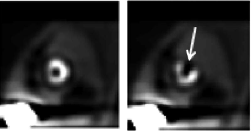
The simulated noisy projection data were reconstructed using filtered back-projection (FBP) and a ramp filter with cut-off at the Nyquist frequency. The reconstructed voxels were cubic with a side length of 0.442 cm. We reconstructed 48 transaxial slice region centered on the heart, resulting in a 128×128×48 reconstructed image matrix. The reconstructed images were filtered with a 3-D Butterworth filter of order 8 at cut-off frequencies 0.08, 0.1, 0.12, 0.14, 0.16, 0.2 and 0.24 cycle per pixel. The filtered images were reoriented into a standard short-axis orientation (Frey et al., 2002, Ghaly et al., 2015, Elshahaby et al., 2015a) and a 64×64 image centered on the position of the defect for the defect-present class or the corresponding defect location for the defect-absent class was extracted and windowed (Frey et al., 2002, Gilland et al., 2006, Ghaly et al., 2015, He et al., 2004, He et al., 2010, He et al., 2006). In the windowing step, negative values were set to zero, values that were larger than or equal to the maximum value in the heart were set to 255 and the remaining values were mapped to the range [0, 255]. Lastly, the resulting floating-point values were rounded to integers. Figure 1 shows the resulting noise-free short-axis defect-absent and defect-present images.
Fig. 1.
Noise-free short-axis images with the image on the left represents the defect-absent case and on the right represents the defect-present case. The arrow points to the defect, where the defect shown has severity of 100% for visualization purpose.
3.3. Application of the Frequency-Selective Channel Model
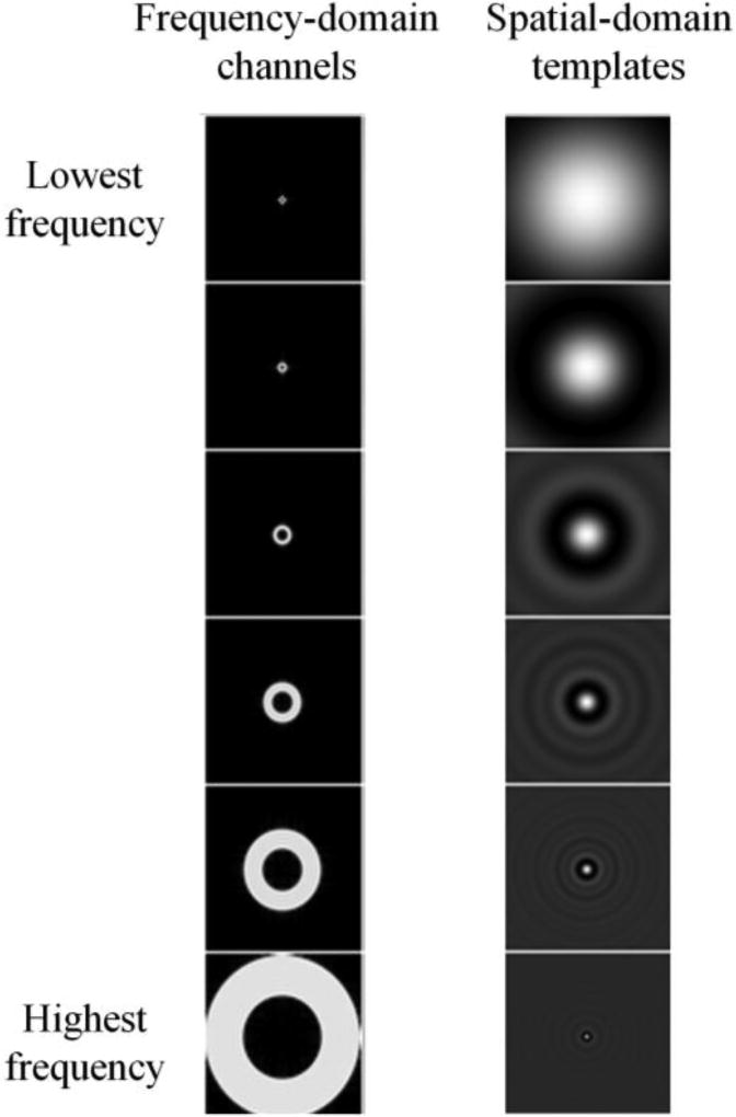
A set of 6 rotationally symmetric channels (Myers and Barrett, 1987) were used as shown in Figure 2. The rotationally symmetric channel model has been widely used in similar tasks involving the assessment and optimization of different nuclear medicine systems using myocardial perfusion images (Wollenweber et al., 1999, Frey et al., 2002). In particular, for the MPS images, the rankings of the systems using the CHO were in good agreement with the rankings of human observers (Wollenweber et al., 1999). In the frequency domain, these channels were non-overlapping passbands having square profile with cut-offs of , and cycle per pixel. The 2D frequency domain channels were transformed analytically to the spatial domain and sampled at the image voxel size. The DC component for each channel was explicitly removed by subtracting the mean value of the spatial domain template (Frey et al., 2002, Elshahaby et al., 2016). The dot product of the post-processed image with each of the spatial domain templates produced a 6×1 feature vector for each image. This process resulted in 2000 pairs of feature vectors (or channel output vectors) for the defect-absent and defect-present classes.
Fig.2.
Images of the six rotationally symmetric frequency-domain channels (left) and the corresponding spatial-domain templates (right).
3.4. Feature Vector Ensembles
We described above the ensemble of feature vectors generated from realistic MPS data. We refer to the underlying distribution of these feature vectors as F-MPS. As observed in (Elshahaby et al., 2016), the probability distribution of theses feature vectors is not consistent with a multivariate Normal (MVN) distribution. The HO and linear discriminant (LD) have performance equal to the ideal observer (IO) when applied to data that are MVN distributed with equal covariance matrices under both hypotheses; the quadratic discriminant has the same performance as the IO when the data are MVN distributed and the covariance matrices are not necessarily equal (Fukunaga, 1990). Since the MVN assumption was violated with the considered dataset, the performance of all 3 observers applied to the feature vector data is expected to be sub-optimal.
Based on the above discussion and for completeness, we also generated data from 2 additional ensembles whose members were drawn from synthetic distributions (MVN with equal and unequal covariance matrices) to test the various observers and resampling schemes.
Both synthetic distributions modeled the mean and covariance of the feature vectors in F-MPS. We estimated these by calculating the sample mean vectors and the covariance matrices , where i denotes the class (i ∈ {1,2,}), from the available 2000 feature vectors from each class. The first synthetic ensemble, F-MVUNEQ, was created by generating 2000 feature vectors for each class using an MVN distributed random-number generator, where the parameters of the MVN distribution were and for the ith class. The second synthetic ensemble, F-MVNEQ, was modeled by generating 2000 feature vectors for each class using an MVN distributed random number generator, where the parameters of the MVN distribution were and for the ith class. These two ensembles represented the cases of MVN data with unequal and equal covariance matrices, respectively.
We generated multiple realizations of each of the above ensembles of feature vectors in order to provide estimates of the precision of the AUC or correlation coefficient, and thus allow computation of the MSE. For F-MPS, we generated 1000 bootstrap samples by drawing random samples of size 2000 (with replacement) from the full set of the available 2000 feature vectors of each class. For the F-MVUNEQ and F-MVNEQ, we repeated the process of generating feature vectors to generate 1000 ensembles of 2000 feature vectors for each class.
A major focus of this work was to investigate the performance of the various methods when using small ensembles of feature vectors. For each of the three full ensembles described above, we created a number of smaller ensembles. To do this, we selected the first n samples from each of the 1000 repetitions, where the ensemble size (number of samples per class) was n ∈ {20, 30, 40, 50, 70, 100, 150, 200, 500, 1000, and 2000}.
3.5. Resampling Schemes and Model Observers
In this work, we investigated if the accuracy and precision of task performance for an observer operating on an ensemble of feature vectors depended on the resampling scheme used to generate the test statistics. In this context, a resampling scheme is the method for selecting feature vectors used to train (i.e., calculate the 1st and 2nd order statistics) and test (i.e., apply the observer to obtain a set of test statistics) the observer. In this work, we used the HT/HT and the LOO (Fukunaga, 1990) schemes. These resampling schemes have been used in nuclear medicine, where the CHO was used with the HT/HT scheme in (He et al., 2004, He et al., 2010, He et al., 2006) and with the LOO scheme in (Frey et al., 2002, Ghaly et al., 2015, Sgouros et al., 2011).
In the first resampling scheme used, the HT/HT, assume a dataset of size 2n, where n is the number of feature vectors per class. In this case, half of the feature vectors from both classes were used to train the observer by computing the 1st and 2nd order statistics of the data and the observer was tested using each feature vector in the other half. This resulted in test statistics per class.
In the second resampling scheme, the LOO scheme (Fukunaga, 1990), 2n experiments were carried out. For each experiment, one feature vector was held out and the remaining 2n − 1 feature vectors were used to estimate the 1st and 2nd order statistics of the data. Then, the held-out vector was used to compute the corresponding test statistic. By holding out a different vector each time, we obtained n test statistics per class.
Since the feature vectors were used by the observers to get the corresponding test statistics, we refer to the observers as the CHO, channelized Linear discriminant (CLD), and channelized Quadratic discriminant (CQD).
3.6. ROC Analysis and Comparison of Observers
The obtained test statistics were analyzed by the ROC-kit software package to estimate the AUC values (Metz et al., 1998, http://metz-roc.uchicago.edu/). For each observer, the mean AUC value for an ensemble size of 2000 samples (i.e., feature vectors) per class served as a gold standard for that observer. Since we are interested in the performance of the observers as a function of ensemble size n, we computed the mean square error (MSE) of the AUCs defined as:
| (7) |
where was the mean AUC for the Jth observer over the 1000 bootstrap repetitions at 2000 samples per class (i.e., the gold standard), and was the AUC for the Jth observer at n samples per class from the ith bootstrap repetition.
We also compared the different combinations of observers and resampling schemes based on the mean Spearman’s rank correlation coefficient R, defined as (Daniel, 1990):
| (8) |
where was the rank correlation coefficient for the Jth observer at n samples per class and was the rank correlation coefficient between the gold standard and the AUC for the Jth observer at n samples per class and from the ith bootstrap repetition. A mean rank correlation coefficient closer to 1 implies a greater ability to correctly rank the performance for the various cut-offs on average. A smaller standard error of the rank correlation coefficient implies that there is a good estimation of the mean of the rank correlation coefficient over the ensembles.
3.7. Comparison Between the Combinations [CHO, LOO] and [CLD, LOO]
To understand the behavior of the two combinations [CHO, LOO] and [CLD, LOO], we conducted the following study using the full set of the available 2000 feature vectors per class of the F-MPS ensemble.
Step1: Calculate the test statistics
From the available 2000 feature vectors per class, we held out one feature vector from each class and randomly drew 1999 samples with replacement from the remaining 1999 feature vectors of each class. This random sampling was done 1000 times. From each of the 1000 repetitions, we selected the first n − 1 samples from each class. Each observer was trained using the selected n − 1 samples from one class and n samples (i.e., the selected n − 1 samples and the held-out sample) from the other class and then tested with the remaining held-out sample. By holding out a different sample each time, we obtained 2000 test statistics for each class. We tried two cases: n = 20 and 2000. This process was repeated 1000 times.
Step2: Evaluate the differences between observers
The root mean square difference (RMSD) in the test statistics gave an indication about the difference between the test statistics estimated using small ensemble size (i.e., 19 samples from one class and 20 samples from the other class were used for training) and the estimated test statistics using large ensemble size (i.e., 1999 samples from one class and 2000 samples from the other class were used for training). The RMSD in the test statistics RMSD(ti) for an observer under the ith hypothesis was calculated from the combined data, as the square root of the average of the squared difference between the estimated test statistics using the small ensemble size and the large ensemble size, over all 2000 test statistics and 1000 repetitions. The RMSD is given mathematically by the following:
| (9) |
where and represent the kth test statistic from the jth bootstrap index, under the ith hypothesis, calculated from the large and small ensemble sizes, respectively. Table 1 shows a list of the abbreviations used and the corresponding description.
Table1.
A summary of the abbreviations and the corresponding description.
| Abbreviation | Description |
|---|---|
| CHO | Channelized Hotelling observer |
| CLD | Channelized Linear discriminant |
| CQD | Channelized Quadratic discriminant |
| HT/HT | Half Train/Half Test resampling scheme |
| LOO | Leave-one-out resampling scheme |
| MVN | Multivariate Normal |
| MPS | Myocardial perfusion SPECT |
| F-MPS | Ensemble of feature vectors generated from realistic MPS data |
| F-MVNEQ | Ensemble of feature vectors generated from MVN distribution with the same covariance matrix under both hypotheses |
| F-MVNUNEQ | Ensemble of feature vectors generated from MVN distribution with unequal covariance matrices under both hypotheses |
| AUC | Area under the ROC curve |
| MSE | Mean square error of the estimated AUC values |
4. Results
4.1. Validation of the Number of Samples Used for Gold Standard
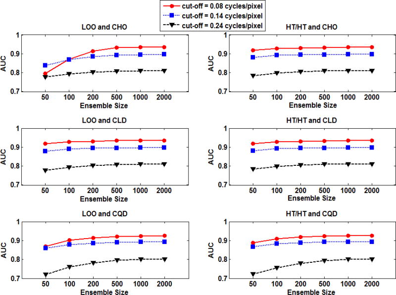
In this work, it was assumed that the mean AUC value for an ensemble size of 2000 samples per class served as a gold standard. Thus, it was important to validate that using 2000 samples per class was sufficient. For this purpose, different ensemble sizes, ranging from 50 to 2000, were used to train and test each of the three observers described in section 2. This process was repeated for the 1000 bootstrap repetitions. Then, the means from the 1000 bootstrap AUC values were calculated for each obsever. The AUC values as a function of ensemble size from the F-MPS ensemble at the lowest, middle, and highest cut-off frequencies are shown in Figure 3. For all six combinations of observers and resampling methods, the estimated AUC values appeared to converge as the ensemble size increases. This observation was true for the other two distributions: F-MVNEQ and F-MVNUNEQ (not shown). To quantify convergence, we computed the percentage change in the mean AUC value from an ensemble size of 1000 (i.e., ) compared to ensemble size of 2000 (i.e., ) for observer J:
| (10) |
Fig. 3.
AUC values obtained for different combinations of observers and resampling schemes as functions of ensemble size (i.e., number of samples/class). The AUC plots represent the mean of 1000 bootstrap repetitions using the F-MPS ensemble.
For F-MPS, the percentage difference in the mean between AUCs at ensemble sizes 1000 and 2000 was less than 0.3% for all observers and resampling schemes.
In order to determine how variable the mean of the AUC was, we drew random resamples of size nresample=1000 with replacement from the available 1000 AUCs. This process was repeated 1000 times. For each of these repetitions, we calculated the mean of the AUC. The standard deviation of the estimated means was computed to measure the variability in the mean of the AUC. The standard deviation of the mean of the AUC was much smaller (less than or equal to ~ 4×10⁻³) relative to the mean. This observation was true for all 7 cut-offs, 11 ensemble sizes, 3 observers, 2 resampling schemes, and 3 distributions.
The combination of the small change in the mean AUC from 1000 to 2000 and the small standard deviations of the mean AUCs justified the use of the AUC value computed from 2000 samples from each class as a gold standard for judging the AUCs estimated from smaller ensemble sizes.
4.2 Effect of Ensemble Size on Observer Performance
In this section, we studied the effect of ensemble size on the performance of the observers for each of the three ensembles: F-MPS, F-MVNEQ, and F-MVUNEQ.
4.2.1. Effect of Ensemble Size on Observer Performance using the F-MPS Ensemble
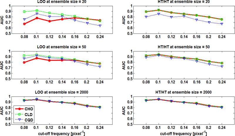
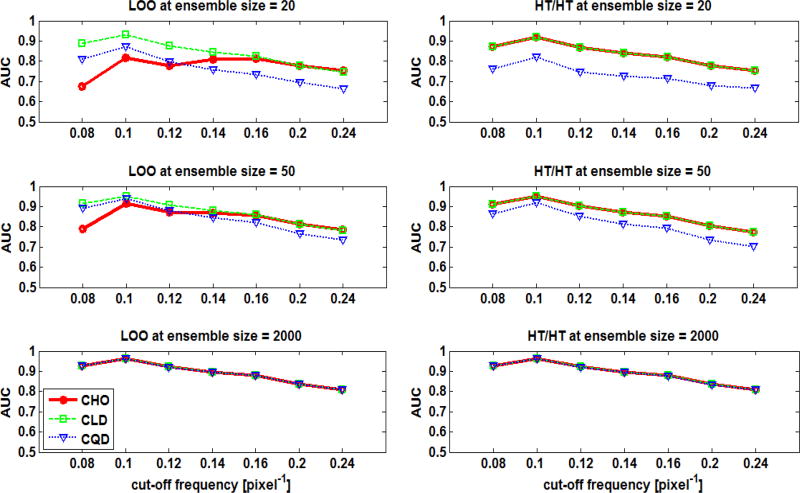
The estimated AUC values as function of the cut-off frequency of the post-reconstruction filter using the F-MPS distribution are shown in Figure 4. The obtained AUCs for the three observers using both resampling techniques were similar at large ensemble size (i.e., 2000 samples/class). This was true for all the cut-off frequencies. However, the performance of the observers diverged as the ensemble size decreased. The smaller ensemble sizes resulted in negatively biased AUCs for all six combinations. Using the HT/HT scheme, the CHO and the CLD gave the same AUCs. However, the performance of CHO and CLD was different for small ensembles when the LOO scheme was used.
Fig. 4.
The estimated mean AUC values as functions of the cut-off frequency of the post-reconstruction filter using the F-MPS ensemble. The plots are for the different six combinations of observers and resampling schemes using various ensemble sizes.
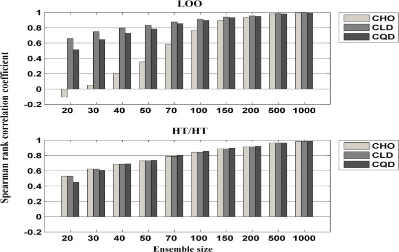
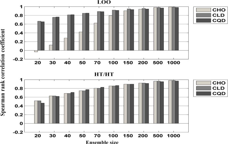
Figure 5 shows the MSE of the estimated AUCs as function of the ensemble size at the middle cut-off frequency (i.e., 0.14 cycle/pixel). Using the LOO scheme at ensemble sizes smaller than 50, the CLD provided the smallest MSE, followed by the CQD, and the largest MSE was obtained when the CHO was used. Figure 6 shows the MSE as a function of the cut-off frequency for an ensemble size of 20 samples/class. The combinations that provided the smallest and almost constant MSEs for the different frequencies were the [CLD,LOO], the [CHO, HT/HT], and the [CLD,HT/HT]. Using the LOO scheme with the CHO for an ensemble size of 20 gave MSE values that varied from ~ 1% to ~7%. When the MSE for different cut-offs at small ensembles was near constant, this implied that the ranking of the cut-offs was less affected by the small ensemble size. The performance rankings for the filter cut-offs, measured by the Spearman’s rank correlation coefficient R, are shown in Figure 7. Using an ensemble size ≥ 200 resulted in R values close to one (i.e., larger than 0.91) for all observers and resampling schemes. For smaller ensemble sizes, the rankings of the cut-offs frequencies were presereved best by the combination [CLD, LOO], followed by [CQD, LOO].
Fig. 5.
The MSE of the estimated AUC values using the F-MPS ensemble as functions of the ensemble size for a cut-off of 0.14 cycle/pixel.
Fig. 6.
The MSE of the estimated AUC values using the F-MPS ensemble as functions of the cut-off frequency for an ensemble size of 20 samples/class.
Fig. 7.
The Spearman’s rank correlation coefficients of the AUCs as functions of the ensemble size using the F-MPS ensemble. The plots represent the mean of the 1000 bootstrap repetitions. The standard error was approximately in the order of 10−4 to 10−2 and is thus not displayed.
4.2.2. Effect of Ensemble Size on Observer Performance Using the F-MVNEQ Ensemble
Figures 8–11 show the results for the F-MVNEQ ensemble. The observers had similar performances for both F-MPS and F-MVNEQ ensembles for most combinations and ensemble sizes.
Fig. 8.
The estimated mean AUC values as functions of the cut-off frequency of the post-reconstruction filter using the F-MVNEQ ensemble. The plots are for the different six combinations of observers and resampling schemes using various ensemble sizes.
Fig. 11.
The Spearman’s rank correlation coefficients of the AUCs as functions of the ensemble size using the F-MVNEQ ensemble. The plots represent the mean of the 1000 bootstrap repetitions. The standard error was approximately in the order of 10−4 to 10−2 and is thus not displayed.
4.2.3. Effect of Ensemble Size on Observer Performance Using the F-MVNUNEQ Ensemble
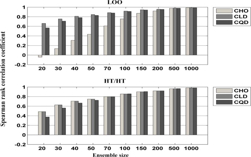
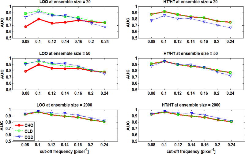
Figures 12–15 show the results for the F-MVNUNEQ ensemble. At ensemble size of 2000, the CQD outperformed the CHO and the CLD for some cut-off frequencies and for both resampling schemes as shown in Figure 12. For smaller ensemble sizes, the observers had almost similar performances to those from the F-MPS and F-MVNEQ ensembles.
Fig. 12.
The estimated mean AUC values as functions of the cut-off frequency of the post-reconstruction filter using the F-MVNUNEQ ensemble. The plots are for the different six combinations of observers and resampling schemes using various ensemble sizes.
Fig. 15.
The Spearman’s rank correlation coefficients of the AUCs as functions of the ensemble size using the F-MVNUNEQ ensemble. The plots represent the mean of the 1000 bootstrap repetitions. The standard error was approximately in the order of 10−4 to 10−2 and is thus not displayed.
4.3. Comparison Between the Combinations [CHO, LOO] and [CLD, LOO]
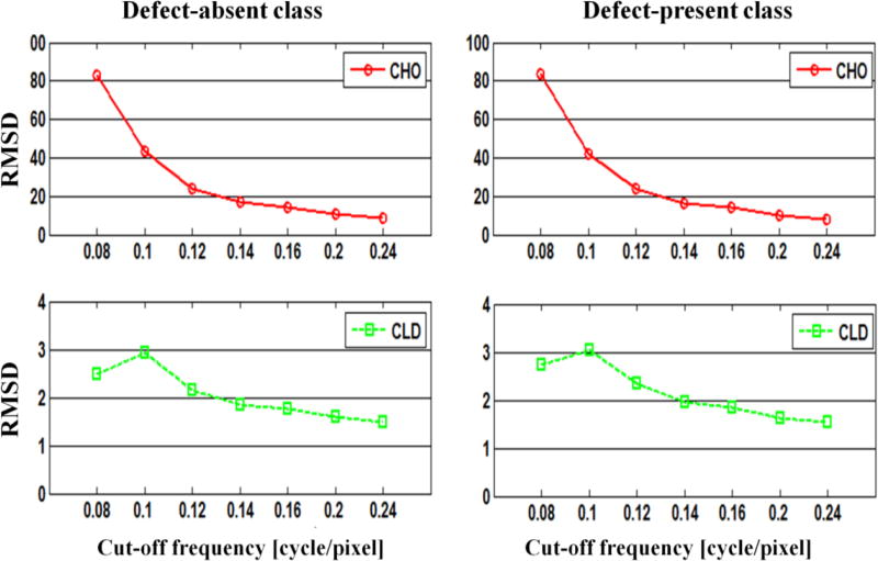
The RMSD of the estimated test statistics for both the CHO and the CLD are shown in Figure 16. The RMSD using the CHO was much larger than that using the CLD, especially for lower cut-off frequencies. This observation was true for both the defect-absent and defect-present class. This indicates that the RMSD in the test statistics estimated from the smaller ensemble was larger for the CHO than for the CLD when using the LOO resampling scheme. This additional error in test statistic values can explain the large difference in the estimated AUCs between CHO and CLD at lower cut-offs, when small ensemble size was used (see Figure 4).
Fig. 16.
The RMSD of the estimated test statistics using the F-MPS ensemble. Note that the vertical scale is smaller by a factor of 25 for the CLD compared to the CHO.
5. Discussion
It has been assumed in the literature that the performance of the CHO and the CLD is the same (Myers and Barrett, 1987) because the difference between the test statistics from these two observers is the extra term Δ defined in eq. (6); which is independent of the test data. In this work, it was demonstrated that the use of the CLD with the described LOO scheme has major advantages in the case of a binary classification task when small ensembles of MPS images, with only uptake variability, were used.
The performances of all observers (as measured by the AUC values) were similar at large ensemble sizes, except the CQD that outperformed the CHO and the CLD for the F-MVNUNEQ data at some cut-offs. To explain this, recall that the CQD will have optimal performance (i.e., equal to the performance of the IO) when the data from the two classes are MVN distributed with unequal covariance matrices, which was the case of F-MVNUNEQ data at large ensemble size (Chan et al., 1999). The CLD and the CHO will be suboptimal in the case of F-MVNUNEQ because of the unequal covariance matrices.
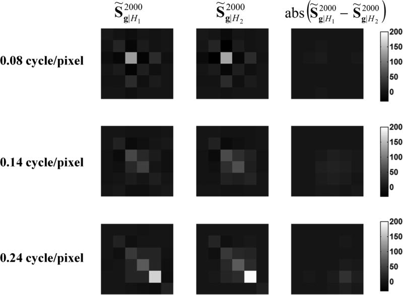
Figure 17 shows images of the covariance matrices for both classes, and images of their absolute difference at cut-offs 0.08, 0.14, and 0.24 cycle/pixel. It is observed from Figure 17 that the covariance matrices of the two classes had different structures and this difference in structure changed as a function of the cut-off frequency. This could explain why the CQD had higher AUC values than the CHO and CLD for some cut-offs at large ensemble size (see Figure 12, bottom row).
Fig. 17.
Images of the covariance matrices for the defect-absent (left column) and the defect-present (middle column) classes, and images of the absolute difference between the covariance matrices (right column).
The results reported in section 4 showed that, in general, the CQD required larger ensemble size than that required by the CLD. Our observations were consistent with previous findings present in Refs.(Wahl and Kronmal, 1977, Marks and Dunn, 1974, Fukunaga, 1990).
Although we have used the rotationally symmetric channels with square profile, the analysis and principles developed in this work can be applied to other channel types. However, further experiments are necessary to draw conclusions about the different channel models, especially for the case of [CLD, LOO] and [CHO, LOO].
In this work, the goal was to find a strategy (i.e., an observer and a resampling scheme) that provides an improved precision for small ensemble sizes. Thus, we used an ensemble size of 2000 samples/class as our gold standard and we did not model internal noise in the observer. To match the human observer performance, internal noise can be added (Brankov, 2013). The work presented in this paper could be extended to include internal noise in the test statistics calculations. We anticipate that the addition of internal noise can change the underlying AUC values, but the precision of the AUC estimates may not be that much affected.
5.1 Comparison between the CHO and CLD
As the ensemble size decreased, the AUC values became more negatively biased for all observers and data distributions. It was observed that the CLD observer trained and tested using the described LOO scheme gave better performance for small ensemble sizes, regardless of the distribution of the data (see Figures 4 to 15). In other words, this combination better preserved the AUC values because the MSE was small and almost constant over the different frequencies (see Figures 5, 6, 9, 10, 13, and 14). Consequently, the rankings of the cut-off frequencies were better preserved (see Figures 7, 11, and 15).
Fig. 9.
The MSE of the estimated AUC values using the F-MVNEQ ensemble as functions of the ensemble size for a cut-off of 0.14 cycle/pixel.
Fig. 10.
The MSE of the estimated AUC values using the F-MVNEQ ensemble as functions of the cut-off frequency for an ensemble size of 20 samples/class.
Fig. 13.
The MSE of the estimated AUC values using the F-MVNUNEQ ensemble as functions of the ensemble size for a cut-off of 0.14 cycle/pixel.
Fig. 14.
The MSE of the estimated AUC values using the F-MVNUNEQ ensemble as functions of the cut-off frequency for an ensemble size of 20 samples/class.
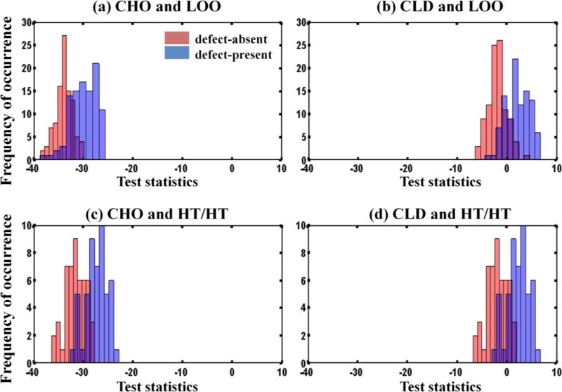
Although the CHO and the CLD are both linear classifiers and the only difference between them is the extra term Δ defined in eq. (6), their numerical behavior depends on the training and testing scheme. Figure 18 shows the histograms of the test statistics using 100 samples/class. It is observed that the extra term in the CLD affected the shape of the distribution of the test statistics compared to that of the CHO, for the LOO scheme (see Figures 18 (a) and (b)). However, the same was not true for the HT/HT scheme (see Figures 18 (c) and (d)). The extra term Δ depends on the mean vectors and covariance matrices of the data computed during the training phase. For the HT/HT scheme, this term was computed once from half the available samples and then used to calculate the test statistics for the remaining samples. Thus, the distribution of the test statistics using CLD will be a shifted version of that obtained using CHO. For the LOO scheme, the extra term was computed for each of the 2n experiments (as previously described in section 3.5). This would result in 2n different values of Δ and each test statistic was calculated using a different Δ. Thus, the distribution of the test statistics using CLD will not be only a shifted version of that obtained using CHO, but the shape of the distribution may also be different.
Fig. 18.
Histograms of the test statistics of the CHO and the CLD using both resampling schemes for the F-MPS ensemble using 100 samples/class.
6. Conclusions
In this work, we assessed the performance of three channelized model observers: CHO, CLD, and CQD, using two resampling schemes: leave-one-out (LOO) and half train/half test (HT/HT), for different ensemble sizes.
For the task considered, the results showed that the combination [CLD, LOO] better preserved the performance rank for small ensembles, followed by either the [CQD, LOO], the [CHO, HT/HT] or [CLD, HT/HT]. The combination [CHO, LOO] had the worst performance both in terms of preserving AUC and performance rank for small ensemble size. The performance of CHO and CLD were the same when HT/HT resampling was used, as expected. The combination [CQD, HT/HT] had higher MSE than the [CHO, HT/HT] and [CLD, HT/HT] combinations for the small ensembles, likely reflecting the larger number of parameters that must be estimated from the training set. These observations held for all three datasets investigated.
The results of this study suggest that CLD combined with the LOO scheme is more able to handle small ensemble sizes for SKE/BKS task evaluation than the other methods investigated. The use of this combination has the potential to provide more statistical power for a given number of images, and thus allow for the study of a larger range of parameters in optimization studies.
Acknowledgments
This work was supported by National Institutes of Health grants R01 EB016231 and R01 EB013558. The content is solely the responsibility of the authors and does not necessarily represent the official views of the National Institutes of Health.
References
- Barrett HH, Myers KJ. Foudations of Image Science. New York: Wiley; 2004. [Google Scholar]
- Barrett HH, Yao J, Rolland JP, Myers KJ. Model observers for assessment of image quality. Proc. Natl. Acad. Sci. USA. 1993;90:9758–9765. doi: 10.1073/pnas.90.21.9758. [DOI] [PMC free article] [PubMed] [Google Scholar]
- Brankov JG. Evaluation of the channelized Hotelling observer with an internal-noise model in a train-test paradigm for cardiac SPECT defect detection. J. Phys. Med. Biol. 2013;58:7159–82. doi: 10.1088/0031-9155/58/20/7159. [DOI] [PMC free article] [PubMed] [Google Scholar]
- Chan HP, Sahiner B, Wagner RF, Petrick N. Classifier design for computer-aided diagnosis: effects of finite sample size on the mean performance of classical and neural network classifiers. Med Phys. 1999;26:2654–68. doi: 10.1118/1.598805. [DOI] [PubMed] [Google Scholar]
- Daniel WW. Applied nonparametric statistics. Cengage Learning; 1990. [Google Scholar]
- Elshahaby FEA, Ghaly M, Jha AK, Frey EC. The effect of signal variability on the histograms of anthropomorphic channel outputs: Factors resulting in non-Normally distributed data. Proc. SPIE on Medical Imaging. 2015a;9416 [Google Scholar]
- Elshahaby FEA, Ghaly M, Jha AK, Frey EC. Factors affecting the normality of channel outputs of channelized model observers: An investigation using realistic myocardial perfusion SPECT images. J. Med. Img. 2016;3:015503. doi: 10.1117/1.JMI.3.1.015503. [DOI] [PMC free article] [PubMed] [Google Scholar]
- Elshahaby FEA, Ghaly M, Li X, Jha AK, Frey EC. Estimating model observer performance with small image ensembles. J. Nucl. Med. 2015b;56(supplement 3):540–540. [Google Scholar]
- Frey EC, Gilland KL, Tsui BM. Application of task-based measures of image quality to optimization and evaluation of three-dimensional reconstruction-based compensation methods in myocardial perfusion SPECT. IEEE Trans. Med. Imaging. 2002;21:1040–50. doi: 10.1109/TMI.2002.804437. [DOI] [PubMed] [Google Scholar]
- Fukunaga K. Introduction to Statistical Pattern Recognition. Academic Press; 1990. [Google Scholar]
- Fukunaga K, Hayes RR. Effects of sample size in classifier design. IEEE Trans. on Pattern Analysis and Machine Intelligence. 1989a;11:873–885. [Google Scholar]
- Fukunaga K, Hayes RR. Estimation of classifier performance. IEEE Trans. Pattern Anal. Mach. Intell. 1989b;11:1087–1101. [Google Scholar]
- Ge D, Zhang L, Cavaro-Ménard C, Gallet PL. Numerical stability issues on channelized Hotelling observer under different background assumptions. J. Opt. Soc. Am. A. 2014;31:1112–1116. doi: 10.1364/JOSAA.31.001112. [DOI] [PubMed] [Google Scholar]
- Ghaly M, Du Y, Fung GS, Tsui BM, Links JM, Frey E. Design of a digital phantom population for myocardial perfusion SPECT imaging research. Phys. Med. Biol. 2014;59:2935–53. doi: 10.1088/0031-9155/59/12/2935. [DOI] [PMC free article] [PubMed] [Google Scholar]
- Ghaly M, Du Y, Links JM, Frey EC. Collimator optimization in myocardial perfusion SPECT using the ideal observer and realistic background variability for lesion detection and joint detection and localization tasks. Phys Med Biol. 2016;61:2048–2066. doi: 10.1088/0031-9155/61/5/2048. [DOI] [PMC free article] [PubMed] [Google Scholar]
- Ghaly M, Links JM, Frey EC. Optimization of energy window and evaluation of scatter compensation methods in myocardial perfusion SPECT using the ideal observer with and without model mismatch and an anthropomorphic model observer. J. Med. Img. 2015;2 doi: 10.1117/1.JMI.2.1.015502. [DOI] [PMC free article] [PubMed] [Google Scholar]
- Gifford HC, King MA, De Vries DJ, Soares EJ. Channelized hotelling and human observer correlation for lesion detection in hepatic SPECT imaging. J. Nucl. Med. 2000;41:514–21. [PubMed] [Google Scholar]
- Gilland KL, Tsui BMW, Qi Y, Gullberg GT. Comparison of channelized hotelling and human observers in determining optimum OS-EM reconstruction parameters for myocardial SPECT. IEEE Transactions on Nuclear Science. 2006;53:1200–1204. [Google Scholar]
- He X, Frey EC, Links JM, Gilland KL, Segars WP, Tsui BM. A mathematical observer study for the evaluation and optimization of compensation methods for myocardial SPECT using a phantom population that realistically models patient variability. IEEE Trans Nucl Sci. 2004;51:218–224. [Google Scholar]
- He X, Links JM, Frey EC. An investigation of the trade-off between the count level and image quality in myocardial perfusion SPECT using simulated images: the effects of statistical noise and object variability on defect detectability. Phys Med Biol. 2010;55:4949–61. doi: 10.1088/0031-9155/55/17/005. [DOI] [PMC free article] [PubMed] [Google Scholar]
- He X, Links JM, Gilland KL, Tsui BM, Frey EC. Comparison of 180 degrees and 360 degrees acquisition for myocardial perfusion SPECT with compensation for attenuation, detector response, and scatter: Monte Carlo and mathematical observer results. J. Nucl. Cardiol. 2006;13:345–53. doi: 10.1016/j.nuclcard.2006.03.008. HTTP://METZ-ROC.UCHICAGO.EDU/ [DOI] [PubMed] [Google Scholar]
- Kupinski MA, Clarkson E, Hasterman JY. Bias in Hotelling Observer Performance Computed from Finite Data. Proc Soc Photo Opt Instrum Eng. 2007;6515:1–7. doi: 10.1117/12.707800. [DOI] [PMC free article] [PubMed] [Google Scholar]
- Marks S, Dunn OJ. Discriminant Functions When Covariance Matrices are Unequal. Journal of the American Statistical Association. 1974;69:555–559. [Google Scholar]
- Metz CE, Herman BA, Shen J-H. Maximum likelihood estimation of receiver operating characteristic (ROC) curves from continuously-distributed data. Statistics in Medicine. 1998;17:1033–1053. doi: 10.1002/(sici)1097-0258(19980515)17:9<1033::aid-sim784>3.0.co;2-z. [DOI] [PubMed] [Google Scholar]
- Myers KJ, Barrett HH. Addition of a channel mechanism to the ideal-observer model. J. Opt. Soc. Am. A. 1987;4:2447–57. doi: 10.1364/josaa.4.002447. [DOI] [PubMed] [Google Scholar]
- Park S, Clarkson E, Kupinski MA, Barrett HH. Efficiency of human and model observers for signal-detection tasks in non-Gaussian distributed lumpy backgrounds. Proceedings SPIE Medical Imaging 2005: Image Perception, Observer Performance, and Technology Assessment. 2005a;5749:138–149. Year. [Google Scholar]
- Park S, Clarkson E, Kupinski MA, Barrett HH. Efficiency of the human observer detecting random signals in random backgrounds. J Opt Soc Am A Opt Image Sci Vis. 2005b;22:3–16. doi: 10.1364/josaa.22.000003. [DOI] [PMC free article] [PubMed] [Google Scholar]
- Sahiner B, Chan HP, Hadjiiski L. Classifier performance prediction for computed-aided diagnosis using a limited dataset. Med. Phys. 2008;34:1559–1570. doi: 10.1118/1.2868757. [DOI] [PMC free article] [PubMed] [Google Scholar]
- Sankaran S, Frey EC, Gilland KL, Tsui BM. Optimum compensation method and filter cutoff frequency in myocardial SPECT: a human observer study. J. Nucl. Med. 2002;43:432–8. [PubMed] [Google Scholar]
- Sgouros G, Frey EC, Bolch WE, Wayson MB, Abadia AF, Treves ST. An approach for balancing diagnostic image quality with cancer risk: application to pediatric diagnostic imaging of 99mTc-dimercaptosuccinic acid. J. Nucl. Med. 2011;52:1923–1929. doi: 10.2967/jnumed.111.092221. [DOI] [PMC free article] [PubMed] [Google Scholar]
- Tseng HW, Fan J, Kupinski MA. Design of a practical model-observer-based image quality assessment method for x-ray computed tomography imaging systems. J Med Imaging (Bellingham) 2016;3 doi: 10.1117/1.JMI.3.3.035503. [DOI] [PMC free article] [PubMed] [Google Scholar]
- Wahl PW, Kronmal RA. Discriminant Functions when Covariances are Unequal and Sample Sizes are Moderate. Biometrics. 1977;33:479–484. [Google Scholar]
- Wollenweber SD, Tsui BMW, Lalush DS, Frey EC, Lacroix KJ, Gullberg GT. Comparison of Hotelling observer models and human observers in defect detection from myocardial SPECT imaging. IEEE Transactions on Nuclear Science. 1999;46:2098–2103. [Google Scholar]
- Wunderlich A, Noo F. Estimation of Channelized Hotelling Observer performance with known class means or known difference of class means. IEEE Trans. Med. Imaging. 2009;28:1198–1207. doi: 10.1109/TMI.2009.2012705. [DOI] [PMC free article] [PubMed] [Google Scholar]
- Yihuan L, Lin C, Gene G. Collimator performance evaluation for In-111 SPECT using a detection/localization task. Physics in Medicine and Biology. 2014;59:679. doi: 10.1088/0031-9155/59/3/679. [DOI] [PubMed] [Google Scholar]


