Nth-order linear algorithm for diffuse correlation tomography

Abstract

The current approaches to imaging the tissue blood flow index (BFI) from diffuse correlation tomography (DCT) data are either an analytical solution or a finite element method, both of which are unable to simultaneously account for the tissue heterogeneity and fully utilize the DCT data. In this study, a new imaging concept for DCT, namely NL-DCT, was created by us in which the medical images are combined with light Monte Carlo simulation to provide geometrical and heterogeneous information in tissue. Moreover, the DCT data at multiple delay time are fully utilized via iterative linear regression. The unique merit of NL-DCT in utilizing the medical images as prior information, when combined with a split Bregman algorithm for total variation minimization (Bregman-TV), was validated on a realistic human head model. Computer simulation outcomes demonstrate the accuracy and robustness of NL-DCT in localizing and separating the flow anomalies as well as the capability to preserve edges of anomalies.

1. Introduction

Near-infrared diffuse optical spectroscopy (NIRS) is one of the major approaches to in vivo probe tissue blood oxygenation parameters, including oxy- and deoxy-hemoglobin concentrations (Δ[HbO2], Δ[Hb]), total hemoglobin concentration (THC) and oxygen saturation (StO₂) [1–5]. A derived technology, namely, the diffuse optical tomography (DOT), has also been developed for decades to localize oxygenation in diseased organs or tissues such as tumors, brain and skeletal muscles [6–8]. DOT measurement requires the placements of an array, containing a large number of source-detector (S-D) pairs, on the tissue surface, and an algorithm is used to reconstruct the 3D oxygenation imaging through modeling of diffusive light. The propagation of diffusive light can be modeled by a partial differential equation (PDE) [7], or alternately, it is described by the Monte Carlo simulation of light propagation, which typically involves millions of photons migrations [9,10]. Mathematically, the DOT is considered as an inverse problem and mostly solved by the PDE-based approaches [11]. At early stage, analytical solution to PDE was utilized for DOT image reconstruction, wherein a regular geometry (e.g., semi-infinite, cylinder, sphere, etc.) was assumed. However, the complicated geometry and tissue heterogeneity of biological tissue are difficult to be taken into consideration by analytical solution. Hence, another solution for PDE, i.e., the finite element method (FEM), is becoming more popular in recent years [7,12]. Consequently, open-source FEM software, such as Nirfast (www.nirfast.org) and TOAST + + (http://web4.cs.ucl.ac.uk/research/vis/toast/), were established and public available, which triggered the widely clinical applications of DOT.

The DOT for oxygenation imaging, however, only provides a single and static parameter of the oxygen kinetics. Blood flow is such a parameter that reflects the dynamic balance between the oxygen supply and consumption [13,14]. Moreover, combination of blood flow and oxygenation permits estimate of oxygen metabolic rate [15], a direct indicator of many diseases. Over years, a dynamic NIRS technology, namely, the diffuse correlation spectroscopy (DCS) [16,17], or diffusing wave spectroscopy (DWS) [18,19], has been developed and applied in various tissues. DCS utilizes the temporal autocorrelations of light electric field (g₁(τ)) at multiple delay time (τ) to quantify the moving of red blood cells, offering an innovative way to directly monitor microvascular blood flow change over time. Apart from this, quantification of spatial flow contrast is likewise important, which triggered the development of a new flow imaging technology, namely, the diffuse correlation tomography (DCT).

Similar to DOT, the early stage of DCT imaging algorithm is also based on the analytical solution [20,21]. This method shares the same limit as difficult to account for irregular tissue geometry. To overcome this limit, the FEM-based DCT algorithm has been proposed [22], and it was applied to intralipid phantom as well as human breast tumors with irregular geometry [22,23]. As a brief summary, analytical solution and FEM are the current methods of flow imaging for DOT and DCT. The two methods, when being applied to DCT, only the autocorrelation data (g₁(τ)) at a single delay time (τ) is utilized for image reconstruction, which is susceptible to the noise of autocorrelation data.

To account for the tissue heterogeneity and irregular geometry, a sort of N-order linear (NL) algorithms were recently proposed by us as an alternate solution for DCS [24,25]. Unlike analytical solution and FEM, NL algorithm doesn’t seek for the solution to PDE. Instead, it combines the integral form of g₁(τ) with a Nth-order Taylor polynomial, and the tissue heterogeneity and irregular geometry are fully taken into account through the information of photon trajectory. More importantly, the unique merit of NL algorithm, in contrast to the PDE solutions (i.e., analytical solution or FEM), is that the autocorrelation function (g₁(τ)) at multiple delay time are fully utilized, which could generate more robust blood flow indices. The accuracy and robustness of NL algorithm for DCS have been validated through computer simulations and mouse stroke experiment [24,25].

Translation of NL algorithm from DCS to DCT for flow imaging, however, is not straightforward and involves complicated procedures. Unlike the DCS that utilizes few S-D pairs, the DCT needs an array, containing a large number of S-D pairs, to be placed on the target tissue. More importantly, the coefficient matrix derived from DCT algorithm is ill-posed, requiring efficient approaches for accurate and robust image reconstruction. Additionally, the unbalanced signal-to-noise (SNR) levels among S-D pairs, due primarily to the difference in the distances between the source and detector, substantially affect the quality of the reconstructed flow images. Based on the NL algorithm, we established in this article, for the first time to the best of our knowledge, a new DCT framework that is distinct from PDE models, for full utilization of autocorrelation data. Furthermore, an established approach for image reconstructions, namely, the Split Bregman algorithm for total variation minimization (Bregman-TV), was incorporated with the NL-DCT to enhance the accuracy and robustness of flow imaging. The capability of the proposed DCT framework for restoration of flow anomaly, particularly on the location and edge preservation, was extensively validated through computer simulations on a realistic human head.

2. Methods

This section starts with introduction of the traditional algorithms for DCT flow imaging, including the analytical solution and FEM. We then elaborated on the NL-DCT framework that was proposed by us, including the NL algorithm for DCT flow imaging, image reconstruction algorithm, tissue model of human head, the setup for source-detector pairs and anomalies, as well as the procedures to generate original DCT data. At the end of this section, we compared the outcomes derived from the full (i.e., multiple delay time) and partial (i.e., single delay time) utilizations of DCT data, which are adopted by NL-DCT and traditional algorithms, respectively.

2.1 Traditional algorithms for DCT flow imaging

The current algorithms for DCT flow imaging are analytical solution and FEM, both of which are derived from the below diffusion correlation equation ([21] and [22]).

$$\nabla \left(\left(\frac{D(r)}{v}\right)\nabla G_1(r,\tau )\right)-\left({\mu }_a(r)+\frac{1}{3}{\mu }_s^{\text{'}}(r)k_0^2\alpha 〈\Delta r^2(\tau )〉\right)G_1(r,\tau )=-S(r)e^{i\frac{2\pi \tau c}{\lambda }}$$ (1)

Here, G₁(r,τ) is the unnormalized electric field temporal autocorrelation function. r is the position vector, v is the light speed in the medium, λ is the wavelength, μ_a is the medium absorption coefficient, $D(r)\approx v/3{\mu }_s^{\text{'}}$ is the medium photon diffusion coefficient, and S(r) is continuous-wave isotropic source.

The solutions to Eq. (1) with analytical method has the following form [21]:

$${\phi }_{\mathrm{s}}(r_{si},r_{di},\tau )=\text{ln}\frac{g_1(r_{si},r_{di},\tau )}{g_{1,0}(r_{si},r_{di},\tau )}={\displaystyle \sum _{j=1}^N{W}_{\mathit{\text{ij}}}(r_{si},r_{di},r_j,\tau )}\Delta (\alpha D_B(r_j))$$ (2)

Here the W_ij is the coefficient matrix that can be calculated from the Green’s function in the homogeneous medium by diffusion correlation equation. ${\phi }_s\left(r_{si},r_{di},\tau \right)$ is the autocorrelation function g₁(τ) in heterogeneous medium that is normalized to its homogeneous value, collected from ith S-D pair. The dynamic changes of blood flow index (BFI) (i.e., Δ(αD_B(r_j)) is derived by solving linear equation system Eq. (2).

The FEM solution to diffusion correlation equation Eq. (1) is similar to that of the standard DOT equation (see reference [7] for details), except that the measurement data is the autocorrelation function g₁(τ) rather than the light intensity. By defining a dynamic absorption term (i.e.,${\mu }_{\mathrm{a}}^d(r,\tau )=\frac{1}{3}{\mu }_s^{\text{'}}(r)k_0^2\alpha 〈\Delta r^2(\tau )〉=2{\mu }_s^{\text{'}}(r)k_0^2\alpha D_B(r)\tau$) in Eq. (1), the absolute value of BFI (i.e., αD_B(r)) is readily derived, once the ${\mu }_{\mathrm{a}}^d(r,\tau )$ is calculated from the standard FEM for DOT [22].

The two methods, when being applied to DCT, only the autocorrelation data (g₁(τ)) at a single delay time (τ) is utilized for image reconstruction, which is susceptible to the noise of autocorrelation data.

2.2 NL algorithm for DCT flow imaging

The NL-DCT proposed by us is a brand new modeling for DCT flow imaging that is paralleled to the existing analytical solution and FEM. Based on the previous efforts on DCS/DCT principles [25], we proposed a NL algorithm solely for DCT, namely NL-DCT, in the following details. Assuming that we have M sources (m = 1,…, M) to launch photons into tissue and have J detectors (j = 1,…, J) to collect the photons escaped from tissue. The target tissue is meshed with n elements in space. The temporal autocorrelation g₁(τ) from the (mth, jth) source-detector pair can be treated as the integral of the autocorrelation decay from individual photon travelling through different elements, as expressed in below form:

$$\begin{array}{l}{g}_1(m,j,\tau )=\frac{<E(m,j,0)E^{*}(m,j,\tau )>}{<{\left|E(m,j,0)\right|}^2>}\\ ={\displaystyle {\int }_0^{\infty }P(m,j,s_1,\mathrm{...},s_n)\text{exp}}(-\frac{1}{3}{\displaystyle \sum _{i=1}^n{k}_0^2(i)<\Delta r_i^2(\tau )>\frac{s_i}{l_i^{*}})}\mathrm{d}(s_1,\mathrm{...},s_n)\\ ={\displaystyle {\int }_0^{\infty }P(m,j,s_1,\mathrm{...},s_n)\text{exp}(-2}{\displaystyle \sum _{i=1}^n{k}_0^2(i)\alpha D_B(i)s_i{\mu }_s^{\text{'}}(i)\tau })\mathrm{d}(s_1,\mathrm{...},s_n)\end{array}$$ (3)

Here P(m,j,s₁,…,s_n) is the normalized distribution of detected photon path length over n elements, k₀(i) is the wave vector magnitude of the light in ith element, $l_i^{*}$is the photon random-walk step length in ith element, which is equal to $1/{\mu }_s^{\text{'}}(i)$ (${\mu }_s^{\text{'}}(i)$ is the reduced scattering coefficient in ith element), and τ is the delay time of autocorrelation function. $<\Delta r_i^2(\tau )>$is the mean-square-displacement of the moving scatters in ith element. $<\Delta r_i^2(\tau )>$ can have different forms. From the previous experimental results, $<\Delta r_i^2(\tau )>=6\alpha D_B(i)\tau$ was found to fit the real DCS/DCT data well. The combined term αD_B(i) denotes the blood flow index (BFI) in ith element.

Mathematically, the continuous function g₁(m,j,τ) can be expressed as the form of N-order Taylor polynomial:

$$\begin{array}{l}\hfill g_1(m,j,\tau )=g_1(m,j,0)+g_1^{(1)}(m,j,0)\tau +{\displaystyle \sum _{k=2}^N\frac{g_1^{(k)}(m,j,0)}{k!}{\tau }^k}+\hfill \\ \hfill \frac{g_1^{(N+1)}(m,j,\xi ){\tau }^{N+1}}{(N+1)!},(0<\xi <\tau )\hfill \end{array}$$ (4)

Combing Eq. (3) with Eq. (4) and performing the similar procedures described in our previous report [25], we obtain the first-order (N = 1) and Nth-order (N>1) approximations when τ is sufficient small, as follows.

$$g_1(m,j,\tau )-1=\tau {\displaystyle {\int }_0^{\infty }P(m,j,s_1,\mathrm{...},s_n)[-2{\displaystyle \sum _{i=1}^n{k}_0^2(i)\alpha D_B(i)s_i{\mu }_s^{\text{'}}(i\text{)]}}}d(s_1,\mathrm{...},s_n)$$ (5)

$$\begin{array}{l}{g}_1(m,j,\tau )-\text{1-}{\displaystyle \sum _{k=2}^N\frac{{\displaystyle {\int }_0^{\infty }P(m,j,s_1,\mathrm{...},s_n){[-2{\displaystyle \sum _{i=1}^n{k}_0^2(i)\alpha D_B(i)s_i{\mu }_s^{\text{'}}(i)}]}^k}d(s_1,\mathrm{...},s_n)}{k!}{\tau }^k}\\ =\tau {\displaystyle {\int }_0^{\infty }P(m,j,s_1,\mathrm{...},s_n)[-2{\displaystyle \sum _{i=1}^n{k}_0^2(i)\alpha D_B(i)s_i{\mu }_s^{\text{'}}(i)}]}d(s_1,\mathrm{...},s_n)\end{array}$$ (6)

For computer implementation, we discretize the above formula, resulting in below forms of first-order (N = 1) and Nth-order (N > 1) approximations.

$$g_1(m,j,\tau )-1=\tau {\displaystyle \sum _{i=1}^{n}B(m,j,i)}\alpha D_B(i)$$ (7)

$$\begin{array}{l}{g}_1(m,j,\tau )-1-{\displaystyle \sum _{k=2}^N\frac{{{\displaystyle \sum _{q=1}^{Q}w(q,m,j)\left(-2{\displaystyle \sum _{i=1}^n{k}_0^2(i)\alpha D_B(i)s(i,q,m,j){\mu }_s^{\text{'}}(i)}\right)}}^k}{k!}}{\tau }^k\\ =\tau {\displaystyle \sum _{i=1}^{n}B(m,j,i)}\alpha D_B(i)\end{array}$$ (8)

Here

$$B(m,j,i)={\displaystyle \sum _{q=1}^Q-2w(q,m,j)k_0^2(i)s(i,q,m,j){\mu }_s^{\text{'}}\left(i\right)}$$ (9)

The w(q,m,j), termed as photon weight in literature, is the discretization of P(m,j,s₁,…s_n), in which the qth photon (q = 1,…, Q) packet has the path length (s₁,…,s_n) over n elements. s(i,q,m,j) denotes the s_i path length corresponding to qth photon packet in (mth,jth) S-D measurement. Both w(q,m,j) and s(i,q,m,j) can be estimated from the Monte Carlo simulation of light propagation in heterogeneous tissue and with arbitrary geometry.

For computing convenience, we convert the two-dimensional index (m, j) into one-dimensional index h (h = 1,…, MJ) according to the equation: h = j + (m-1)J, and then define:

$$A\left(h,i\right)=B\left(m,j,i\right)$$ (10)

$$\alpha D_B={\left[\alpha D_B(1),\alpha D_B(2),\dots \alpha D_B\left(n\right)\right]}^{\mathrm{T}}$$ (11)

Thus, A is a matrix of MJ × n dimensions. αD_B is a vector of n × 1 dimensions.

When the order N = 1, the unknown variables αD_B only appear in the right-hand side of Eq. (7). Hence, Eq. (7)can be rewritten as follow:

$$g_1(h,\tau )-1=\tau {\displaystyle \sum _{i=1}^{n}B(m,j,i)}\alpha D_B^{(1)}(i)=\tau {\displaystyle \sum _{i=1}^{n}A(h,i)}\alpha D_B^{(1)}(i)=\tau (A\ast \alpha {D_B}^{(1)})$$ (12)

The term A*αD_B⁽¹⁾ is the slope of linear regression between τ and g₁(h,τ)-1, which is rewritten as:

$$A\ast \alpha {D_B}^{(1)}=Sl$$ (13)

Once the slope (Sl) is determined from τ and g₁(h,τ)-1 data via linear regression, the unknowns (αD_B⁽¹⁾) can be calculated from Eq. (13) with proper image reconstruction algorithm.

When the order N > 1,the unknown variables αD_B appear in both sides of Eq. (8). Hence, the calculation of BFIs is implemented in iterative procedures. The final form of solution is:

$$\begin{array}{l}\hfill g_1(h,\tau )-1-{\displaystyle \sum _{k=2}^N\frac{{{\displaystyle \sum _{q=1}^{Q}w(q,\mathrm{h})\left(-2{\displaystyle \sum _{i=1}^n{k}_0^2(i)\alpha {D_B}^{(N-1)}(i)s(i,q,h){\mu }_s^{\text{'}}(i)}\right)}}^k}{k!}}{\tau }^k\hfill \\ \hfill =\tau {\displaystyle \sum _{i=1}^{n}A(h,i)}\alpha {D_B}^{(N)}(i)=\tau (A\ast \alpha {D_B}^{(N)})\hfill \end{array}$$ (14)

$$A\ast \alpha {D_B}^{(N)}=S{l}^{(N)}$$ (15)

2.3 Image reconstruction algorithm

For the NL-DCT imaging framework that is created by us, the major computation procedures include the linear regressions to obtain the slopes (Eq. (12) and Eq. (14)) and the solving of linear equation system (Eq. (13) and Eq. (15)) to reconstruct the BFIs. The linear regression between the delay time (τ) and the modified autocorrelation function (i.e., the left-hand side of Eq. (12) or Eq. (14)) can be readily implemented through least-squares approach, and the higher-order iteration would result in more accurate approximation.

Similar to DOT, the S-D pairs (i.e., measurement number) are far less than the unknowns (i.e., αD_B^(N)), leading to a severely ill-posed inverse problem of Eq. (13) and Eq. (15). Hence, adoption of constrains and regularizations to solve the linear equation system is the primary challenges for computation implementation of flow imaging.

In field of diffuse optical imaging, Tikhonov regularization is the primary tool used for image reconstruction [7]. However, Tikhonov regularization is designed to seek for the optimal balance between the L₂ norm minimization and data fidelity. The L₂ norm minimization, however, does not well reflect the sparse representation of medical image when compared with the lower-order norm minimization such as L₁ and L₀. Over the last decade, the total variation (TV) has been emerging as a regularization term to reconstruct medical imaging from sparsely measured data, particularly in community of computed tomography (CT) research [26]. The TV regularization aims for sparse representation of images through minimizing the L₁ norm of image gradient magnitude transform. As for solving TV minimization, the split Bregman algorithm has been proved to be an efficient approach and utilized for DOT reconstruction [27]. Hence, this approach is adopted by us in this article and abbreviated as Bregman-TV. Below is a brief description of the Bregman-TV procedures.

In Eq. (13) and Eq. (15), let v = αD_B^(N), b = Sl^(N). Hence, target function of the Bregman-TV proposed for NL-DCT is expressed in the following form.

$$\begin{array}{l}{v}^{*}=\text{arg min}{\Vert v\Vert }_{TV}+\frac{\mu }{2}{\Vert Av-b\Vert }_2^2\\ \text{s.t.}{v}_i\ge 0(i=1,2,\mathrm{...},n)\end{array}$$ (16)

Here, non-negativity of solutions is enforced.

The TV norm form that is based on anisotropic gradient transform of a 3D image can be expressed as:

$${\Vert v\Vert }_{TV}={\Vert \nabla \nu (x,y,z)\Vert }_1={\Vert {\nabla }_x\nu \Vert }_1+{\Vert {\nabla }_{\mathrm{y}}\nu \Vert }_1+{\Vert {\nabla }_z\nu \Vert }_1$$ (17)

Here

$$\begin{array}{l}{\left({\nabla }_{x}v\right)}_{i,j,k}=v_{i+1,j,k}-v_{i,j,k}\\ {\left({\nabla }_{y}v\right)}_{i,j,k}=v_{i,j+1,k}-v_{i,j,k}\\ {\left({\nabla }_{z}v\right)}_{i,j,k}=v_{i,j,k+1}-v_{i,j,k}\end{array}$$ (18)

Through variable substitutions, the optimization problem Eq. (16) is transformed into:

$$\begin{array}{l}\underset{v,d_x,d_y,d_z}{\text{min}}{\Vert d_x\Vert }_1+{\Vert d_y\Vert }_1+{\Vert d_z\Vert }_1+\frac{\mu }{2}{\Vert Av-b\Vert }_2^2\\ \mathit{\text{s.t.}}{d}_x={\nabla }_{x}v,d_y={\nabla }_{y}v,d_z={\nabla }_{z}v\end{array}$$ (19)

Equation (19) can be solved by Bregman split algorithm, as follows:

$$\begin{array}{l}\underset{v,d_x,d_y,d_z}{\text{min}}{\Vert d_x\Vert }_1+{\Vert d_y\Vert }_1+{\Vert d_z\Vert }_1+\frac{\mu }{2}{\Vert Av-b\Vert }_2^2+\\ \frac{\lambda }{2}\Vert d_x-{\nabla }_{x}v-b_x^k\Vert {}_2^2+\frac{\lambda }{2}{\Vert d_{\mathrm{y}}-{\nabla }_{y}v-b_y^k\Vert }_2^2+\frac{\lambda }{2}\Vert d_z-{\nabla }_{z}v-b_z^k\Vert {}_2^2\end{array}$$ (20)

$$b_{\mathrm{x}}^{k+1}=b_x^k+({\nabla }_x{v}^{k+1}-d_x^{k+1})$$ (21)

$$b_y^{k+1}=b_y^k+({\nabla }_y{v}^{k+1}-d_y^{k+1})$$ (22)

$$b_{\mathrm{z}}^{k+1}=b_z^k+({\nabla }_z{v}^{k+1}-d_z^{k+1})$$ (23)

The variables v and d_x, d_y, d_z in Eq. (20) are updated in the following sequences.

Step 1: solve the suboptimization problem for v^k+1

$$\begin{array}{l}{v}^{k+1}=\text{arg}\underset{v}{\text{min}}\frac{\mu }{2}{\Vert Av-b\Vert }_2^2+\frac{\lambda }{2}\Vert d_x^k-{\nabla }_{x}v-b_x^k\Vert {}_2^2+\\ \frac{\lambda }{2}{\Vert d_{\mathrm{y}}^k-{\nabla }_{y}v-b_y^k\Vert }_2^2+\frac{\lambda }{2}\Vert d_z^k-{\nabla }_{z}v-b_z^k\Vert {}_2^2\end{array}$$ (24)

And then enforce non-negativity:

$$v^{\mathrm{k}+1}=\{\begin{array}{ll}{v}^{\mathrm{k}+1}& v^{\mathrm{k}+1}\ge 0\\ 0& v^{\mathrm{k}+1}<0\end{array}$$

Step 2: solve the suboptimization problem for d_x^k+1, d_y^k+1, d_z^k+1

$$\begin{array}{l}(d_x^{k+1},d_y^{k+1},d_z^{k+!})=\text{arg}\underset{d_x,d_y,d_z}{\text{min}}{\Vert d_x\Vert }_1+{\Vert d_y\Vert }_1+{\Vert d_z\Vert }_1+\\ \frac{\lambda }{2}\Vert d_x-{\nabla }_x{v}^{k+1}-b_x^k\Vert {}_2^2+\frac{\lambda }{2}{\Vert d_y-{\nabla }_y{v}^{k+1}-b_y^k\Vert }_2^2+\frac{\lambda }{2}\Vert d_z-{\nabla }_z{v}^{k+1}-b_z^k\Vert {}_2^2\end{array}$$ (25)

Step 3: update b_x^k+1, b_y^k+1, b_z^k+1 according to Eqs. (21)-(23).

If stop criterion:

$${\Vert v^{k+1}-v^k\Vert }_2<\epsilon$$ (26)

does not meet, repeat Step 1 through Step 3.

In step 1, v is updated by Bi-Conjugate Gradients Stabilized (BICGSTAB) algorithm [28]. Step 2 is to calculate d according to the shrinkage algorithm:

$$d_{\mathrm{x}}^{k+1}=\text{shrink}\left(\left|{\nabla }_x{v}^{k+1}+b_x^k\right|,\frac{1}{\lambda }\right)$$ (27)

$$d_y^{k+1}=\text{shrink}\left(\left|{\nabla }_y{v}^{k+1}+b_y^k\right|,\frac{1}{\lambda }\right)$$ (28)

$$d_z^{k+1}=\text{shrink}\left(\left|{\nabla }_z{v}^{k+1}+b_z^k\right|,\frac{1}{\lambda }\right)$$ (29)

Here

$$\text{shrink}\left(t,\gamma \right)=\frac{t}{\left|t\right|}*\text{max}(\left|t\right|-\gamma ,0)$$ (30)

2.4 Tissue model and S-D setup

A realistic human head model was obtained from a MRI image data set that is public available (http://brainweb.bic.mni.mcgill.ca/brainweb/). The size of head model used in this study (i.e., Suject04) is 181 × 217 × 181 mm³, with 0.5 mm spacing in all dimensions. An open-source C + + class library, i.e., visualization toolkit (VTK) version 7.0, was utilized to create 3D visualization platform from the MRI data.

A source-detector (S-D) array was placed on the surface of forehead. The array consists of 9 sources and 28 detectors distributed in rectangular pattern, as shown in Fig. 1. The source and detector are indexed with the number increasing from left to right and from bottom to top. As such, there are a total of 252 S-D pairs. The optical measurements from these S-D pairs (i.e., 252 optical measurements) were used for DCT flow imaging.

Fig. 1.

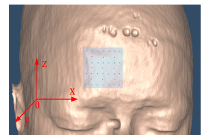
the placement of S-D array on the surface of human forehead.

The original voxels (i.e., elements) contained in human head are: 362 × 434 × 362 = 56,873,096, which is far more than the optical measurements (i.e., 252). Hence, two approaches were adopted to reduce the element number. One approach is to select a small volume from the head and covered it by the S-D array. Another approach is to make the size of element larger than that of original MRI voxel. In this study, a volume of 30 × 30 × 30 mm³ was selected with spacing of 2 mm, 2 mm and 3 mm in x, y and z dimension, respectively, corresponding to15 × 15 × 10 elements. Figure 1 shows the positioning of S-D array on the surface of human forehead.

In order to visualize the 3D flow outcomes in human head with original spatial resolution, the BFI value in each element is registered by adjacent interpolation method into the corresponding original voxel, over the selected volume of 30 × 30 × 30 mm³.

2.5 Anomaly setup

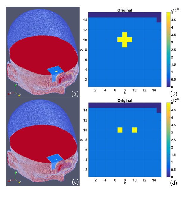
To evaluate NL-DCT’s capability to restore the anomaly shape and location in flow image, a cross-shape anomaly, with a size of ten elements, was placed inside the selected volume, as shown in 2D (Fig. 2(b)) transverse plane and 3D (Fig. 2(a)) human head. Here an open-source software ParaView (Kitware, NY, USA) was adopted by us for outcome visualization.

Fig. 2.

Setup of a cross-shape anomaly (a) and dual cube-shape anomalies (c) in 3D human head (9 mm beneath the forehead surface). (b) and (d) show the two anomaly setup in 2D transverse plane respectively.

The depth of the anomaly center varied from 5 to 15 mm from the head surface. Furthermore, in order to evaluate the capability of NL-DCT for separating different anomalies, a pair of cube-shape anomalies (i.e., dual-anomalies) at spacing of 4 mm were placed inside the selected volume (Fig. 2(c) and Fig. 2(d). Each anomaly has a size of two elements, and the depth was also set from 5 through 15 mm to the surface of the head. The BFI value in all anomalies is set as five-fold of the surrounding tissue (1.0 × 10⁻⁸ cm²/s). The optical properties are assumed as homogeneous all over the head, with the values of absorption coefficient μ_a = 0.1 cm⁻¹, scattering coefficient μ_s = 80 cm⁻¹, anisotropy factor g = 0.9 and refractive index n = 1.37.

2.6 Generation of autocorrelation data

The simulated data of autocorrelation function was generated according to Eq. (3) in discrete form, in which the photon weight w(q,h) and photon path length s(i,q,h) were obtained from the Monte Carlo (MC) simulations of light propagation on the human head. An open-source voxelized type of software (i.e., MCVM [29]) was utilized to perform the MC simulation of light propagation on the original-size of head model. In order to record the photon trajectories in a large number of tissues (each element was treated as an independent tissue) at multiple S-D pairs, substantial amends were made to the codes of MCVM [30]. A total of 10 million photon packets were injected from each source to the head. Primary outcomes from MC simulation, including the photon coordinates, transmission directions, path length, weight (i.e., the remaining ratio of the escaping photons), were used as inputs to Eqs. (7)-(9).

The autocorrelation data were generated by transforming Eq. (3) to its discrete form, as follows:

$$g_1(m,j,\tau )={\displaystyle \sum _{q=1}^{Q}w(q,m,j)\text{exp}\left(-2{\displaystyle \sum _{i=1}^n{k}_0^2(i)\alpha D_B(i)s(i,q,m,j){\mu }_s^{\text{'}}\left(i\right)}\right)}$$ (31)

Together with the variable w(q,,m,j) and s(i,q,m,j) generated by Monte Carlo (MC) simulations, as well as the values of the optical properties (μ_a , μ_s, g and n) and the BFI values assigned in Sections 2.5, we can obtain g₁(h,τ) = g₁(m,j,,τ) from the (m, j) S-D pair.

In actual measurement environment, noise is unavoidable. To better simulate the experiments, the standard deviation of the noise (σ(τ)) was added to autocorrelation function g₁(τ) at each delay time (τ), according to the following equation [31]:

$$\begin{array}{l}\sigma (\tau )=\sqrt{\frac{T}{t}}[{\beta }^2\frac{(1+e^{-2\Gamma T})(1+e^{-2\Gamma \tau })+2m(1-e^{-2\Gamma T})e^{-2\Gamma T}}{(1-e^{-2\Gamma T})}\\ {+2{〈n〉}^{-1}\beta (1+e^{-2\Gamma \tau })+{〈n〉}^{-2}\beta (1+e^{-2\Gamma \tau })]}^{\raisebox{1ex}{$1$}\!\left/ \!\raisebox{-1ex}{$2$}\right.}\end{array}$$ (32)

Here, T is the correlator bin time, Γ is the decay rate, <n> = IT, and I is the detected photon count rate (i.e., light intensity).

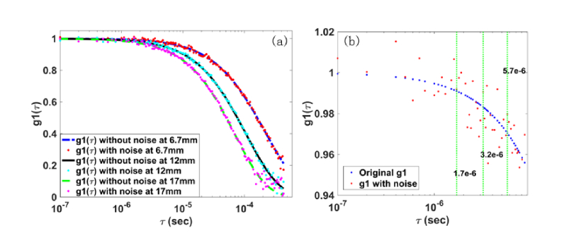
Figure 3(a) shows the autocorrelation curves g₁(τ) with and without noise at the S-D distances of 6.3 mm, 12.0 mm, and 17.0 mm, respectively. As expected, the longer S-D distance leads to faster decay of autocorrelation curve. The noise, primarily dependent on the detected light intensity and the distance of S-D, deviates the g₁(τ) data from the ideal autocorrelation curve.

Fig. 3.

(a) is the curve of autocorrelation g₁(τ, i, j) with and without noise, collected at the S-D separation of 6.3 mm, 12 mm, and 17 mm, respectively.(b) A zoom-in segment of g₁(τ, i, j) curve at the 6.3 mm S-D separation, marked with three representative of single delay time (τ = 1.7 × 10⁻⁶, 3.2 × 10⁻⁶, 5.7 × 10⁻⁶ second [22, 23])

As a preliminary investigation on the accuracy of the proposed NL-DCT for full data utilization, the noisy DCT data at 6.3 mm S-D separation were utilized for comparison between our proposed framework (NL-DCT) and previous methods (analytical solution and FEM). From Eq. (12), the optical measurement by single delay time is defined as: [g₁(τ)-1]/τ, which is equivalent to that by multiple delay time (i.e., the right-hand side on Eq. (13).

When using the single delay time at three representative values (i.e., τ = 1.7 × 10⁻⁶, 3.2 × 10⁻⁶, 5.7 × 10⁻⁶ second [22, 23], see Fig. 3(b)), the mean error of optical measurement averaging over all S-D pairs is 23.1%, 11.8%, 6.3% respectively. By contrast, with multiple delay time (50 time points in the range from τ = 0 to 8.6 × 10⁻⁶ second), the measurement error was substantially decreased to 2.3%. These comparisons demonstrate that the NL-DCT framework could yield more accurate optical measurement through full utilization of data, which is hardly achieved by the analytical solution and FEM.

2.7 Evaluation criteria

Outcomes of the reconstructed flow images by NL-DCT framework will be visually evaluated on the selected volume and the entire head. Additionally, the following two variables were defined for quantitative evaluation.

Root mean squared error (RMSE) quantifies the difference between the reconstructed and true images, and it is defined as follows:

$$\text{RMSE}=\sqrt{\frac{1}{n}{\displaystyle \sum _i^n{(\frac{\alpha D_B^i-\alpha D_{B,0}^i}{\alpha D_{B,0}^i})}^2}}$$ (33)

Here, $\alpha D_B^i$ and $\alpha D_{B,0}^i$are the reconstructed and true BFIs in ith element respectively. n is the number of elements. A small RMSE value indicates that the reconstructed BFI image is close to the true one.

Correlation coefficient (CORR) quantifies the similarity between the reconstructed and true images, and it is defined as follows:

$$\text{CORR}=\frac{{\displaystyle \sum _{i=1}^n\alpha D_B^i\cdot \alpha D_{B,0}^i}}{\sqrt{{\displaystyle \sum _{i=1}^n{(\alpha D_B^i)}^2{\displaystyle \sum _{i=1}^n{(\alpha D_{B,0}^i)}^2}}}}$$ (34)

A large CORR value indicates that reconstructed BFI image is similar to the true one.

3. Results

This section illustrates and evaluates the outcomes of cross-shape and dual cube-shape abnormal BFI images reconstructed by NL-DCT framework and Bregman-TV reconstruction algorithm, from the DCT data without and with noise.

3.1 The reconstructed BFI images using the g₁(τ) without noise

All procedures involved in the BFI image reconstruction, including 3D visualization of human head via VTK, MC simulation of light propagation, as well as solving the linear equation system, were performed on a desktop PC (Lenovo ThinkCentre M8600t-D068), with 3.4G Hz CPU and 16G memory.

For implementation of the image reconstruction algorithm specified by Eqs. (16)-(30), the initial parameters were set as: v⁰ = A^T*b (back projection),$d_x^0=d_y^0=d_z^0=b_x^0=b_y^0=b_z^0=0$. The regularization parameters were set as: μ = 10000, λ = 30, and the stop criterion was set as: ε = 0.0015.

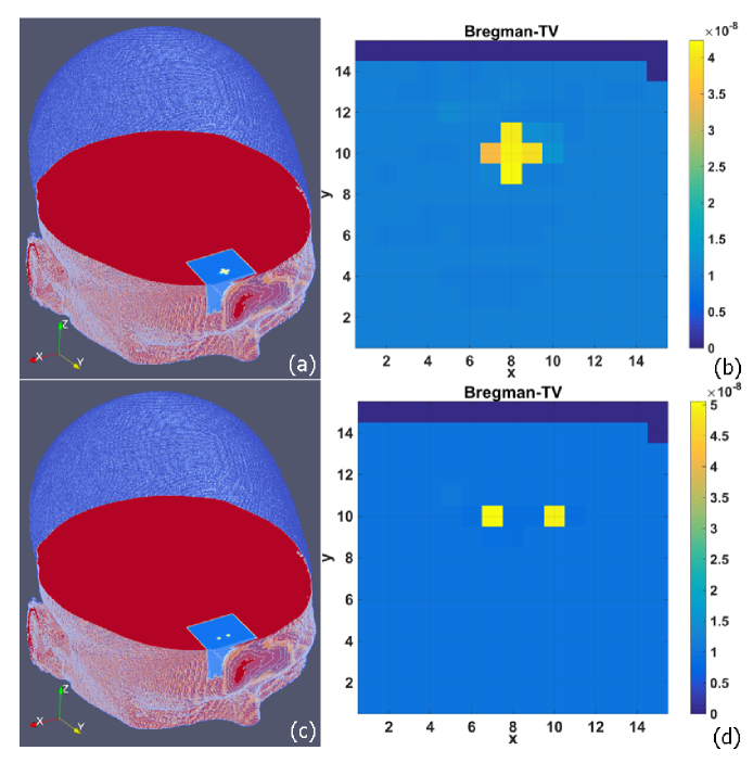
Figure 4 shows the cross-shape and dual cube-shape abnormal BFI images reconstructed by NL-DCT framework. In order to show 3D outcomes, the selected volume (with spacing of 0.2 cm, 0.2 cm and 0.3 cm in x, y and z dimension) is interpolated to the original volume (with spacing of 0.05 cm, 0.05 cm and 0.05 cm in x, y and z dimension) by adjacent interpolation method. Then, the selected volume is mapped back onto the original location in human head.

Fig. 4.

BFI images reconstructed from g₁(τ) data without noise, and shown in 3D volume (a and c) and 2D transverse plane (b and d), respectively . The anomaly is either a cross-shape (a and b) or dual cube-shape (c and d).

It is clearly seen that the shape and location of BFI anomalies are exactly reconstructed and the edge is perfectly preserved. Take the cross-shape anomaly as an example, the RMSE value of BFI over the entire reconstructed image is 0.0769 and the CORR value is 0.988. Generally, the BFI contrast declines with the increase of depth (i.e., along the y axis), which is specifically investigated in Section 3.3. Similarly, the dual anomalies were elegantly separated and the BFI values were more close to the true ones, with RMSE value of 0.0155 and CORR value of 0.999, respectively.

3.2 The reconstructed BFI images using the g₁(τ) with noise

For reconstruction of the flow anomalies with noise defined by Eq. (32), the initial parameters were set as: v⁰ = A^T*b (back projection), $d_x^0=d_y^0=d_z^0=b_x^0=b_y^0=b_z^0=0$. The regularization parameters were set as: μ = 1000, λ = 40, and the stop criterion was set as: ε = 0.005.

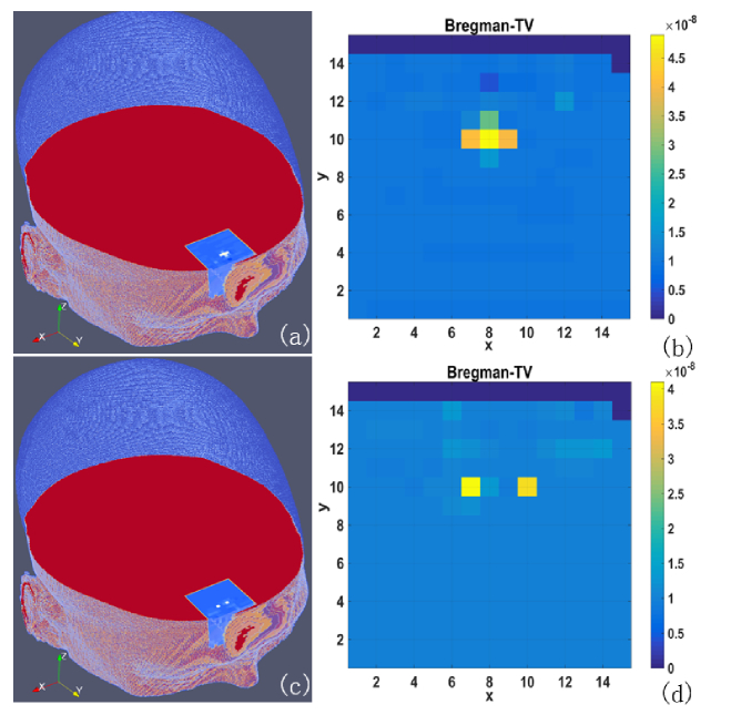
Figure 5 shows the BFI images reconstructed from g₁(τ) data contaminated by noise. When subject to noise, both shape and edge of anomalies are remarkably blurred. Nevertheless, the anomalies are still precisely localized, and the dual anomalies are well separated.

Fig. 5.

BFI images reconstructed from g₁(τ) data with noise, and shown in 3D volume (a and c) and 2D transverse plane (b and d), respectively . The anomaly is either a cross-shape (a and b) or dual cube-shape (c and d).

According to the objective criterion, the RMSE value is 0.153 and the CORR is 0.936 for the cross-shape anomaly. For the dual cube-shape anomalies, the corresponding values of RMSE and CORR are 0.144 and 0.923, respectively.

3.3 Time-course of image reconstructions

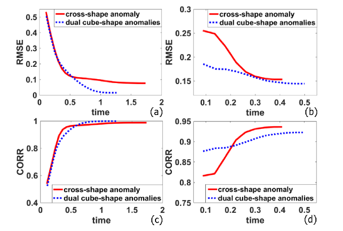
Figure 6 shows the time-course RMSE and CORR of the BFI images that were reconstructed by NL-DCT framework. For both settings of anomalies, the image reconstruction is fairly fast, reaching the convergence value within 1.68 and 1.13 seconds, respectively, for cross-shape and dual cube-shape anomalies. In general, dual cube-shape anomalies lead to the smaller RMSE and higher CORR values, when compared with cross-shape anomaly. The possible reason for this phenomenon is that dual-cube anomalies (four elements with higher value) are more sparse than cross-shape anomaly (ten elements with higher value).

Fig. 6.

Time-course RMSE (a and b) and CORR (c and d) values calculated from the reconstructed images. The outcomes were derived from the g₁(τ) data without noise (a and c) and with noise (b and d). In all sub-figures, the red solid curve denotes the outcomes of cross-shaped anomaly, and blue dotted curve denotes those of dual cube-shape anomalies.

When the noise is added to g₁(τ) data, the value of RMSE increased from 0.0769 to 0.1533, and the value of CORR decreased from 0.988 to 0.936 for cross-shape anomaly. Similar alteration was also found for dual cube-shape anomalies, which is anticipated, because the noise definitely affects quality of the reconstructed images. Note that the values of parameters (μ and λ) vary in accordance with the level of data noise, which affect the convergence speed. Thus, we find that the image reconstruction process from noisy g₁(τ) data is faster than that from noise-free g₁(τ) data.

3.4 Influence of anomaly depth on image reconstructions

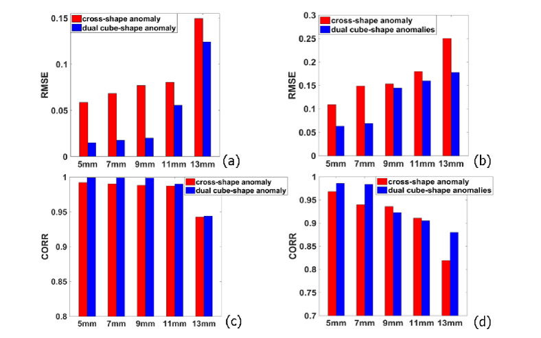
The influence of anomaly depth on the flow image reconstruction is illustrated in Fig. 7. For both cross-shape and dual cube-shape anomalies, the depth is found to have little impact on BFI values when the anomaly is located close to surface (≤ 11 mm). When the anomaly is moving furthermore, however, the BFI errors increase more rapidly than the increase of anomaly depth. Taking the cross-shaped anomaly as an example, the RMSE value increased slightly from 0.0675 to 0.0804 with the depth varied from 5 to 11 mm. However, it increased substantially from 0.0804 to 0.149 with the depth changed from 11 to 13 mm. Additionally, we find that the outcomes of dual-cube anomalies are generally better than cross-shape anomaly. We also attribute the reason to the fact that dual cube-shape anomalies are more sparse than cross-shape anomaly.

Fig. 7.

RMSE and CORR values of reconstructed images as the depth of the anomalies increased. (a) RMSE without noise. (b) RMSE with noise. (c) CORR without noise. (d) CORR with noise. Red is cross-shaped anomaly and blue is two cube-shaped anomalies.

3.5 Influence of anomaly contrast on image reconstructions

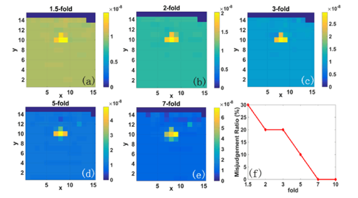
It is worthwhile to examine the influence of anomaly contrast on the reconstructed flow images. For this purpose, the BFI values in anomalies were set by us as 1.5-fold, 2-fold, 3-fold, 5-fold, 7-fold and 10-fold of the BFI values in surrounding tissues. This wide range of anomaly contrast reflects not only most of the diseases causing small flow changes, but also the extreme situations causing larger contrast (e.g., around 10-fold flow contrast in breast cancers [23]).

By using the DCT data with noise, the anomaly with higher contrast exhibits better outcomes of image reconstruction. At 1.5-fold flow contrast, part of the anomaly is hardly visible (Fig. 8(a). By contrast, the whole anomaly is clearly seen in the reconstructed image when the contrast is no less than 5-fold (Fig. 8(d) and 8(e)). Furthermore, we set a value, i.e., 20% higher than the BFI value averaging over the entire volume, as a threshold to judge the anomaly. According to this criterion, the misjudgment ratio for 1.5-fold flow contrast is 30%, and this ratio is decreased to 10% for 5-fold and 0% for 7-fold and 10-fold, respectively (Fig. 8(f)). The outcomes are partially anticipated, since higher flow contrast leads to lower error in determination of anomaly. Note that there are no errors in judging the anomaly location, and the misjudgment ratio is acceptable even if the flow contrast is lowest (i.e., 1.5-fold), indicating the feasibility of NL-DCT for future diagnosis of various diseases.

Fig. 8.

Reconstruction of cross-shape anomaly with varied flow contrast; (a)-(e): the reconstructed images with flow contrast varied from 1.5-fold to 7-fold; (f): the misjudgment ratio of anomaly at different flow contrast.

4. Discussion and conclusions

As a relative new optical technique, DCT has been attracting more attentions in the past decade, for its capability to image microvascular blood flow in noninvasive, rapid and low cost pattern. In addition to the hardware setup (e.g., laser, detector, digital correlator, etc.), the most essential component for DCT is the imaging algorithm, which would remarkably influences the quality of flow images. For a long period, analytical solution of PDE has been used as DCT imaging algorithm, which requires a regular boundary condition (e.g. semi-infinite) that usually does not match the actual tissue geometry. The FEM, which was borrowed from DOT, has applied to DCT in recent years [22, 23], because it takes the irregular tissue geometry into consideration. However, FEM can only utilize the autocorrelation data at single delay time for the DCT image reconstruction, which is susceptible to the measurement noise.

To account for realistic tissue geometry and to fully utilize the autocorrelation data at multiple delay time, we proposed a Nth-order linear (NL) algorithm for DCT image reconstruction in this study. The intrinsic difference between the NL algorithm and the current analytical solution or FEM is that it does not seek for the solution of PDE. Instead, it implements the geometric and heterogeneous information of tissue into the solution via MC simulation of light propagation within the tissues. In the past, the MC simulations are often adopted for the forward solution of diffuse light. In this study, the outcomes of MC simulation, which reflects the irregular geometry and tissue heterogeneity, were utilized by us for solving the inverse problems. Meanwhile, the autocorrelation data at multiple delay time are fully utilized via linear regression, which is difficult to be achieved by the analytical solution and FEM. In principle, thus, the NL algorithm enables precise and robust extraction of the BFI in biological tissues.

The NL-DCT imaging framework was evaluated in this study on a realistic human head characterized by the MRI images that are public available. An open-source VTK was utilized for 3D visualization, through which the S-D array was accurately positioned. Under the NL-DCT imaging framework, the image reconstruction process is aimed to solve an ill-posed linear equation system caused by the unbalance between the unknowns (i.e., BFI elements) and the optical measurements (i.e., S-D pairs). This unbalance could be efficiently alleviated through flexible selections of local volume and meshed with sparse elements, which is uniquely allowed in NL-DCT imaging framework. Consequently, the selected volume of 30 × 30 × 30 mm³, which was meshed with a total of 2250 elements, was mostly covered by the S-D array. Additionally, we reduced the number of elements by excluding those containing little photon trajectory information. Taking together, the number of elements was further reduced by 36.7%, and the accuracy of image reconstruction was improved.

Although the unique innovation of this article is the NL-DCT imaging framework specified in Eqs. (12)-(15), the computing techniques to solve the inverse problem of linear equation system, or in other word, the image reconstruction approach, is also a key factor affecting the image quality. In the past, inverse problems of DOT or DCT were primarily implemented via incorporation with Tikhonov regularization. For other medical imaging modalities such as CT, MRI, PET, however, numerous approaches were well developed, including filtered backprojection (FBP), ART, SART, Maximum-Likelihood Expectation-Maximization (ML-EM), Total Variation (TV) minimization ect, as well as their derived or combined forms. Among these, FBP is an analytical solution capable of fast imaging, thus it is generally utilized for full-view CT. However, this approach is based on central slice theorem that is not met by DCT, because the trajectories of photon migrations are curvatures rather than straight-line.

In fact, most of the image reconstruction methods mentioned above were evaluated in our preliminary studies and thus far, we found Bregman-TV performs best in flows imaging. In order to focus the audience’s attention on the NL-DCT imaging framework that newly created by us rather than the detailed procedures of computing implementations, we only present the outcomes derived from Bregman-TV approach. Nevertheless, many other excellent technologies, including new optimization models, calculating algorithms and sparse representation forms, will be investigated in future works.

Two sorts of flow image setting, i.e., a cross-shape anomaly and dual cube-shape anomalies, were adopted in this study. Although the actual flow images are more complicated, these settings are efficient to test the ability of the proposed approaches for shape and edge preservations, as well as anomaly separation.

Because the optical data collected from large S-D separation (>30 mm) are too weak and contaminated by the noise, the measurements actually being used for image reconstruction are fewer than the theoretical ones (e.g., 252 measurements), which substantially increases difficulty for precise flow imaging. Nevertheless, for the noise-free g₁(τ) data presented in this study, the NL-DCT imaging framework performs excellent in anomaly localization as well as shape and edge restoration. Adding noise to g₁(τ) data, which matches the actual environment of experiments, definitely blurred the shape and edge of anomalies in reconstructed images. Nevertheless, we found that the anomalies were still well localized by NL-DCT. It is expected that the quality of the reconstructed images would be further improved when more S-D pairs are utilized for data collection.

We also roughly compared the outcomes presented in this article with those generated by FEM reported in reference [23]. Although there are differences in the tissue type (head vs. breast) and S-D alignment (rectangular vs. fan), we found that the NL-DCT performs better in the flow contrast error than FEM algorithm (9% vs. 39%) in similar meshing size (~3 mm) and anomaly depth (9 mm vs. 7 mm). Note that, however, this is just a preliminary comparison between the proposed method and previous methods. Solid conclusions requires a wide variations of tissue type, S-D alignment as well as meshing size, which would be carried out in a separate study.

How deep the anomaly can be probed and how fast the flow imaging can be generated are of importance in clinic, where timely diagnosis and medical intervention are preferred. To address these concerns, we particularly investigated the computing time and anomaly depth of the imaging framework. Interestingly, we found there are two stages that characterizes the influence of anomaly depth. When anomaly depth was smaller (≤ 11 mm), its influence on image reconstruction was minor. However, the deep anomaly (> 11 mm) was found to rapidly deteriorate image quality. These outcomes are partially anticipated, because the number of photons within tissues decreases exponentially, rather than linearly, with the increase of tissue depth. Nevertheless, further investigation is needed in order to precisely localize the anomaly in deep tissue such as tumors. As for the imaging speed, the Bregman-TV was found to perform well, leading to quick convergence of flow images.

While excellent outcomes were derived from this study, there are a few possible solutions for improvement of flow imaging. As the first validation example of NL-DCT, a 9 × 28 S-D array was designed by us on human head, and it was shown to well reconstruct the BFI in a volume of 30 × 30 × 30 mm³ with 2-3 mm spatial resolution. In practice, we found that the unbalanced photon path lengths could remarkably affect the image quality. Optimization of S-D configuration will be conducted in the future to minimize the unbalance of photon path lengths. Additionally, the procedures of linear regression involved in the image reconstruction (Eq. (12) and Eq. (14), which is currently based on the L₂ norm minimization, could be further improved via more anti-noise methods. Moreover, it was also found that the quality of flow image is sensitive to the constant parameters involved in the reconstruction approaches, and slight adjustments of parameters values are not totally avoidable. Investigation of parameter options is a part of our ongoing projects.

Although the phantom experiments will enhance the method validation, the computer simulations could guide the experiments prior to probe manufacturing and instrument design, thus substantially reducing the costs. Previous reports with experimental data have demonstrated that the simulated autocorrelation data (i.e., g₁(τ)), along with the realistic noise, matched well with the experimental outcomes [22]. Nevertheless, many factors relevant to the experiments, such as source-detector fiber locations and optical coupling, would significantly affect the flow imaging. A liquid phantom system matching human head geometry, which enables varying the flow speed and anomaly location, is being designed and will be utilized for further validation of NL-DCT approaches.

To conclude, we proposed a NL-DCT framework for flow imaging in this study. Through implement of the photon trajectory information from MC simulation of light propagation, the proposed imaging framework accounts for both irregular geometry and tissue heterogeneity. Moreover, the autocorrelation data at multiple delay time are fully utilized. The NL-DCT framework, when incorporated with Bregman-TV reconstruction approach, was found to be efficient and accurate for flow imaging.

Accelerating the computation speed for real-time imaging, optimization of S-D configuration and image reconstruction approaches via simulation or phantom experiments, as well as their translation to clinic, will be the subjects of future works.

Funding

National Key Research and Development Program of China (2016YFC0101602); National Natural Science Foundation of China (61671413); National Key Scientific Instrument and Equipment Development Project of China (2014YQ24044508); Shanxi Scholarship Council of China (2016-087).

Disclosure

The authors declare that there are no conflicts of interest related to this article.