Supporting Dynamic Quantization for High-Dimensional Data Analytics

Abstract

Similarity searches are at the heart of exploratory data analysis tasks. Distance metrics are typically used to characterize the similarity between data objects represented as feature vectors. However, when the dimensionality of the data increases and the number of features is large, traditional distance metrics fail to distinguish between the closest and furthest data points. Localized distance functions have been proposed as an alternative to traditional distance metrics. These functions only consider dimensions close to query to compute the distance/similarity.

Furthermore, in order to enable interactive explorations of high-dimensional data, indexing support for ad-hoc queries is needed. In this work we set up to investigate whether bit-sliced indices can be used for exploratory analytics such as similarity searches and data clustering for high-dimensional big-data. We also propose a novel dynamic quantization called Query dependent Equi-Depth (QED) quantization and show its effectiveness on characterizing high-dimensional similarity. When applying QED we observe improvements in kNN classification accuracy over traditional distance functions.

ACM Reference format

Gheorghi Guzun and Guadalupe Canahuate. 2017. Supporting Dynamic Quantization for High-Dimensional Data Analytics. In Proceedings of Ex-ploreDB'17, Chicago, IL, USA, May 14-19, 2017, 6 pages. https://doi.org/http://dx.doi.org/10.1145/3077331.3077336

1 Introduction

Exploratory data analysis techniques are used to gather insights from data with the ultimate goal of maximizing the information retrieval quality and the user satisfaction. Data scientists spend much of their time exploring and analysing the data before making further decisions, which eventually leads to enhanced use of a dataset [1].

Data exploration implies that the entire dataset has to be scanned and processed before answering an exploratory query. Furthermore, after an initial set of results, queries are typically refined and have to be answered again. This iterative process makes it difficult to build an effective index for the purpose of data exploration, as the queries are unknown. Thus data exploration can be slow and even unfeasible at times.

Exploratory queries often use a random or user specified seed to execute a similarity search to narrow the exploration over a particular set or subspace of the data. These and other ranked retrieval techniques are applied with the goal of filtering out information. The concept of similarity is captured using a distance function defined over the attributes or features of the data. User preferences can be used to indicate the importance or weight of each feature. However, as the number of features grows, the notion of similarity looses its meaning. The reason is that distances between data points in high-dimensional spaces, are usually very concentrated around their average [5]. This makes it difficult to distinguish between the closest and furthest data points [3].

Distance functions such as PiDist[2], DPF [14], and n-match [15] only consider dimensions that are close to the query point to characterize similarity in high-dimensions. These partial or localized distance functions provide a better distinction between closer and further points and often improve the accuracy of the results. Nevertheless, these distance functions require either expensive preprocessing of the data, or indexing support to be computed efficiently. For high-dimensional data, these indices usually consist of columnar representations of the data such as sorted columns and data quantization.

In our previous work [9] we proposed the use of columnar bit-sliced indices (BSI) to perform preference queries in a distributed environment over high-dimensional data. This approach was shown to outperform other threshold-based algorithms that use sorted columns to perform preference queries. Motivated by this result, in this work we set up to investigate whether this type of index can also be used for exploratory analytics such as similarity searches and data clustering. Creating an index that supports ad-hoc queries can speed up the process of data exploratory analysis. Our first challenge is to devise a way to perform distance computations effectively with this index.

The number of set bits can be used to represent population counts and can be efficiently computed. This opens the door for a novel dynamic quantization which we call Query dependent Equi-Depth (QED) quantization. QED uses the query itself to determine the quantization boundaries. User can specify the number of points desired to fall within the dynamic bin as a percentage of the number of points in the dataset. The query is placed at the center of the bin and the interval is determined to contain at least p points. We evaluate the performance of QED in terms of k-NN classification accuracy over a several labelled datasets, and its robustness to classification parameter k and user-specified parameter p. For all datasets considered in this study, QED was able to improve the baseline classification accuracy.

The rest of this paper is organized as follows. Section 2 presents background and related work. Section 3 describes the index structure and the proposed quantization for similarity searches. Section 4 shows experimental results for classification accuracy. Finally, conclusions and future work are presented in Section 5.

2 Background and Related Work

This section presents background and related work for similarity searches and nearest neighbor queries in high dimensional spaces as well as bit-sliced indices.

2.1 High-dimensional Similarity

Similarity searches are typically posed as nearest neighbor queries, where the k closest points to the query are retrieved as the answer to the query. Manhattan distance is preferred over Euclidean distance for large datasets due to its lower computational cost but no distance metric dominates another in all cases.

Quantization has been widely used to improve the accuracy of classifiers and clustering algorithms as it reduces the noise of the data and simplifies the models. A detail survey of quantization methods can be found in [6]. After quantization, each attribute can be represented using discrete values and points are considered “close” if they fall into the same bin. Hamming distance is the preferred distance metric for discrete domains. In simple terms, the Hamming distance between two data points is the number of dimensions where the two points do not fall into the same bin (or for discrete data, do not have the same value).

Localized similarities only consider a subset of the attributes to compute the distance between high-dimensional data points. Dynamic Partial Function (DPF) [14], considers only the smallest N distances between all the dimensions. To make this method less sensitive to the value of N, the k-N-match algorithm returns the most frequent k objects appearing in the solutions for a range of N values.

In [2], quantization was used to create equi-populated partitions for each dimension and only considered the dimensions for which the two points fall into the same bin to compute the distance. PiDist is defined as:

$$\text{PiDist}(X,Y,k_d)={\left[\sum _{i\in S[X,Y,k_d]}{\left(\frac{|x_i-y_i|}{m_i-n_i}\right)}^p\right]}^{\frac{1}{p}}$$

where k_d is the number of ranges for each dimension, S [X, Y, k_d] is the set of dimensions for which the two objects lie in the same range, and m_i and n_i are the upper and lower bounds of the corresponding range in dimension i. This function accumulates benefit for each attribute for which a data object maps to the same quantization as the query object. It does not differentiate between data and query objects that do not map to the same quantization. Therefore, a data point is not excessively penalized for a few dissimilar attributes. Note that this function is not a distance metric as the triangle inequality property does not hold.

Another approach for high-dimensional similarity is Locality Sensitive Hashing (LSH)[10]. LSH algorithms use data dependent hashing so that similar items fall into the same “bucket”. LSH approaches are extensively used in solving the K-Nearest Neighbors problem. To maximize the probability of retrieving good Nearest Neighbor candidates, one has to generate a high number of hash tables which represents a high storage cost. Due to LSH being an approximate method for similarity searches, we do not compare our approach against it.

2.2 Bit-Sliced Indexing

Bit-sliced indexing (BSI) was introduced in [11] and it encodes the binary representation of attribute values with binary vectors. Therefore, ⎾log₂ values⏋ vectors, each with a number of bits equal to the number of records, are required to represent all the values for a given attribute. This bit-vectors can be compressed using specialized run-length encoding schemes that allow queries to be executed without requiring explicit decompression [7].

BSI arithmetic for a number of operations, including the addition of two BSIs, is defined in [13]. Previous work [9, 12], uses BSIs to support preference and top-k queries efficiently. BSI-based top-k for high-dimensional data was shown to outperform current approaches for centralized queries [9] and distributed environments [8].

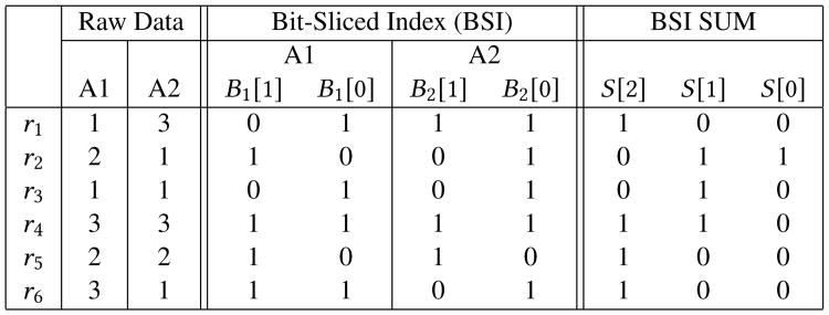
Figure 1 illustrates how indexing of two attribute values and their sum is achieved using bit-wise operations.

Figure 1. Simple BSI example for a table with 6 tuples, two attributes A1 and A2, and three values per attribute.

Since each attribute has three possible values, the number of bit-slices for each BSI is 2. For the sum of the two attributes, the maximum value is 6, and the number of bit-slices is ⎾log₂ 6⏋ = 3. The first tuple t₁ has the value 1 for attribute 1, therefore only the bit-slice corresponding to the least significant bit, B₁[0] is set. For attribute 2, since the value is 3, the bit is set in both BSIs. For example, the addition of the BSIs representing the two attributes is done using efficient bit-wise operations. First, the bit-slice sum[0] is obtained by XORing B₁[0] and B₂[0]: sum[0] = B₁[0]⊗B₂[0]. Then sum[1] is obtained in the following way: sum[1] = B₁[1]⊗B₂[1]⊗(B₁[0]∧B₂[0]). Finally sum[2], which is the carry, is majority(B₁[1], B₂[1], (B₁[0] ∧ B₂[0])), where majority(A, B, C) = (A ∧ B) ∨ (A ∧ C) ∨ (B ∧ C).

We choose this data structure at the basis of our approach due to a number of advantages that we expect to observe in centralized systems as well as in distributed environments. The compact representation of the compressed slices decreases the communication overhead from disk and network between nodes. Bit-wise operations benefit from single instruction multiple data (SIMD) operations. Moreover, breaking up the computation into slices to perform bitwise operations as building blocks for more complex operations provide a greater room for parallelism as all the tasks are independent from each other. Additionally, combination of partial results are very efficient as they do not involve expensive set operations such as union and intersections but rather OR and AND bit-wise operations, respectively.

In this work we do not present a solution for answering nearest neighbor queries in distributed environments using BSI, however that shall be addressed in one of our future works.

3 Proposed Approach

In this section we first provide an overview of how a BSI index can be used to answer Nearest Neighbor queries and then describe the dynamic query dependent equi-depth quantization for high-dimensional similarity.

3.1 kNN queries over BSI

We extended the BSI to handle signed numbers (both 2's complement and sign and magnitude) and represent decimal numbers using a fixed point format for each attribute. For every decimal BSI, the position of the decimal point is maintained as metadata for the attribute. To perform arithmetic operations between two attributes with different precision, namely a and b, where a > b, the decimal point for the second attribute is moved (a – b) positions by multiplying the second attribute by the appropriate power of 10. Multiplication by a constant, as in this case, can be done efficiently by adding the logically shifted BSI to the original BSI for every set bit in the binary representation of the constant. The parallel optimization of the BSI SUM operation over partitioned BSI is presented in [8].

The steps to execute a kNN query over BSI index using Manhattan distance can be summarized as:

1. Compute the distance score between each data point and the query for every dimension. The query point BSI is constructed using compressed bit-vectors of all ones and all zeros and the result is a BSI in 2's complement. The absolute values is computed by XORing every slice with the sign bit-slice and adding the sign slice. The result is an unsigned BSI.

2. Aggregate these BSIs across all dimensions using the parallel operation BSI_SUM [8].

3. Finally, select the k minimum distance scores performing topK-Min operation over the distance BSI (Adapted from [13]).

The steps 1-3 described above are executed using bitwise operations between the bit-vectors of the BSI index. If the bit-vectors are compressed, there is no need for full de-compression. In this work we focus on the dynamic quantization performed during step one described above.

3.2 Query Dependent Equi-Depth Quantization

The similarity function is directly affected by the number of dimensions in the data. The dominant components of distance functions such as the Manhattan or Euclidean metrics are the dimensions on which the points are the farthest apart. With higher dimensionality, the probability of having high discrepancies between two points in at least one dimension increases. The authors of [2, 3] show that for L_p-norm distance functions, the averaging effects of the different dimensions start predominating with increasing dimensionality. To avoid this, the authors of PiDist [2] suggest that by imposing a proximity threshold for each dimension, beyond which the degree of dissimilarity is not relevant, could improve accuracy in nearest neighbor and similarity searches. They achieve this by quantizing the indexed space into a fixed number of bins which are either equi-width or equi-depth (equi-populated). These quantizations are performed over the dataset without considering the query points. Even when a query point lies close to the boundary of a bin, only the points within the bin are considered for computing the similarity.

Algorithm 1: Quantization
	Input: BSI A, int p
	Output: BSI S
1	BitSlice penalty = (A[A.size – 2] XOR A.sign);
2	for (i = A.size – 2;i >= 0;i − −) do
3	penalty = (penalty OR (A[sSize] XOR A.sign));
4	if penalty.count() >= n – p then
5	sSize = i;
6	break;
7	end
8	end
9	BSI S = new BSI(sSize);
10	for (i = 0; i < sSize; i++) do
11	S[i] = (A[i] XOR A.sign);
12	end
13	S.addSlice(penalty);
14	return S

In this work we introduce an equi-depth quantization method that considers the query value for defining the bin boundaries and it is done on-the-fly during query execution. For each dimension, if the data point has its respective dimension within threshold x then the distance to the query is considered for that dimension otherwise a dissimilarity penalty larger than x is assigned. For exploratory tasks, instead of directly specifying x, user specifies parameter p as the minimum number of data points that should be considered in order to define the query bin boundaries. Notice that this is effectively defining equi-populated (equi-depth) ranges for each dimension. Using a population threshold instead of a data value threshold, is motivated by the distribution of real data, which is rarely uniform.

To illustrate the proposed dynamic quantization, consider a 1-dimensional dataset with values:

$$\{\{r1,9\},\{r2,2\},\{r3,15\},\{r4,10\},\{r5,36\},\{r6,8\},\{r7,6\},\{r8,18\}\}$$

and query {q, 10}. If using Manhattan distance, the distance between the data points and the query are:

$$\{\{r1,1\},\{r2,8\},\{r3,5\},\{r4,0\},\{r5,26\},\{r6,2\},\{r7,4\},\{r8,8\}\}$$

For QED, if parameter p = 3, only the 3 points with the smallest distances, i.e. {r1, r4, and r6}, will be considered according to their distance. The rest of the points will be given a larger penalty δ_i to characterize a large dissimilarity. This normalization of the larger differences gives point r5 a chance to make it as a NN in the cases where there are other many dimensions for which r5 is really close to the query. The value of the penalty, δ_i, can be assigned a constant larger than the distances computed within the query-dependent interval for each dimension. In the case of PIDist, the penalty assigned to dissimilar points is 1 and the distance for similar points is normalized to less than 1. Another approach could be to make δ_i to represent a number larger than the largest distance between the query and the closest p elements in dimension i.

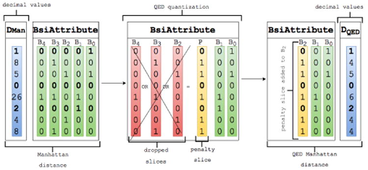
QED can be done gracefully with the BSI index without imposing any overhead when compared to the computation of the Manhattan distance without quantization, as shown in Algorithm 1. Because we operate on top of a BSI index representing the distance between the query and the data points in each dimension, we define the penalty δ_i as the truncation of the most significant bits for the largest distances as depicted in Figure 2.

Figure 2. Query dependent Equi-Depth(QED) quantization with population range p = 3.

QED can be included in the calculation of the absolute value of the distance between query and each dimension as shown in Algorithm 1. In datasets with large attribute ranges, the output of Algorithm 1 is significantly smaller in size than the size of the actual distance measures, for most distributions. This is very important because the result of this operation is further processed to aggregate and rank similar objects. As a result of reducing significantly the output size of this step, the overall execution time of the kNN query is generally improved. The number of bit-vectors required to encode a difference attribute is equal to the number of bits required to encode the difference range. Where the difference range is the maximum difference between the query dimension and the same dimension of any of the p tuples, and their minimum difference.

In large datasets where the number of tuples is high, p should typically be small, and most of those p closest tuples are much closer than the attribute range. Thus the reduction in size of the result of Algorithm 1.

For a better understanding of Algorithm 1, we show how the distance BSI attribute between the query and the data points used in our previous running example is quantized using QED in Figure 2. For simplicity, all the distances are positive in Figure 2 (leftmost BsiAttribute). Starting from the most significant bit-slice, the bit-slices in the distance attribute are OR-ed until the count of set-bits in the resulting bit-slice (the penalty bit-slice) is equal or greater than n – p. At this point the bit-slices that were operated are dropped and replaced with one single penalty bit-slice.

The effect of this quantization is the identification of the furthest n – p points from the query for one given dimension, and reducing their distance, while keeping an accurate distance for the close points. Hence reducing the dissimilarity for outliers and avoiding over penalizing a point if only a few dimensions are far from the query.

Figure 2 and Algorithm 1 use Manhattan distance along with QED quantization. However it is also possible to use other distance metrics such as Euclidean or Hamming.

Equation 1 shows the Hamming distance between a data point a and the query q after applying the QED quantization.

$${\text{QED}}_{\text{Hamming}}(\mathrm{a},\mathrm{q})=\sum _{\mathrm{i}=1}^{\mathrm{d}}\{\begin{array}{cc}0& \text{if}a\in P_i\\ 1& \text{otherwise}\end{array}$$ (1)

Where P_i is the subset of points closest to the query in dimension i.

In the next section we evaluate the QED quantization in terms of classification accuracy over datasets with up to several hundreds of dimensions.

4 Experimental Evaluation

In this section, we perform an experimental evaluation of the kNN classification accuracy for localized distance functions including our query-dependent equi-depth quantization.

We perform experiments over several datasets from the UCI repository [4]. The number of dimensions for the data used in the experiments range from 19 to 279 and the number of classes from 2 to 24. The details of the characteristics of the data and the class distribution can be found in Table 1, as well as on the UCI repository web page.

Table 1. Description of the characteristics of the real datasets used in the experiments.

Dataset	Rows	Cols	Classes (Count per class)
anneal	798	38	5 (8/88/608/60/34)
arrhythmia	452	279	13 (245/50/4/5/22/44/15/15/13/25/3/2/9)
dermatology	366	33	6 (112/61/72/49/52/20)
horse-colic	300	26	2 (99/201)
ionosphere	351	33	2 (126/225)
musk	476	165	2 (269/207)
segmentation	210	19	7 (30/30/30/30/30/30/30)
soybean-large	307	34	19 (1/40/20/10/10/40/20/10/6/6/10/10/40/4/10/40/10/10/10)
wdbc	569	30	2 (357/212)

4.1 Nearest Neighbor Classification Accuracy

For each data set, nearest neighbor (NN) classification is performed for all data points. Classification accuracy is computed over the labeled data using the leave-one-out methodology as the number of correct classifications divided by the total number of tuples in the data set. Voting was used to decide the class for each data point.

Table 2 shows the best classification accuracy when using k-NN classification for each method. We vary the number of nearest neighbors used in classification k = {1, 3, 5, 10, 15, 20, 25}, and report the best result for each distance function. For quantization, we apply Equi-width and Equi-Poplulated partitioning varying the number of bins/clusters from 3 to 20 {3, 5, 7, 10, 15, 20}. The same number of bins/clusters was used for all the dimensions. The only case where attributes could be quantized using a different number of bins/clusters than the one provided as a parameter was the categorical attributes with less categories than the number of bins/clusters provided. In that case each value was considered as a bin/cluster. For dynamic quantization we set p as a percentage of the number of rows. We vary p = {60%, 50%, 40%, 30%, 25%, 20%, 10%, 5%, and 1%}.

Table 2.

Leave-one-out best classification accuracy using k-nearest neighbor (k ∈ {1, 3, 5, 10}) classification with different distance functions and quantization methods (NQ=No Quantization, EW=Equi-witdth, ED=Equi-depth, QED=Query-dependent Equi-depth). The best result for each dataset is highlighted in bold.

		Manhattan		Hamming				PiDist
Dataset	Euc	NQ	QED	NQ	EW	ED	QED	EW	ED
anneal	.934	.939	.964	.986	.984	.980	.994	.990	.990
arrhyt.	.659	.653	.701	.602	.686	.646	.650	.695	.635
dermat.	.975	.978	.986	.975	.973	.883	.921	.981	.970
horse	.740	.770	.783	.780	.827	.857	.867	.833	.843
iono.	.866	.909	.943	.809	.926	.860	.920	.929	.903
musk.	.882	.893	.916	.819	.876	.870	.878	.868	.887
segm.	.843	.886	.881	.586	.871	.857	.924	.900	.876
soyb.	.873	.899	.938	.909	.912	.902	.821	.909	.922
wdbc	.940	.949	.949	.692	.967	.951	.967	.961	.960

The best accuracy for each dataset is highlighted in bold in Table 2. As shown in the table, QED is able to improve the results for Manhattan and Hamming in most datasets. QED using Manhattan is consistently better than Manhattan with no quantization (8/9) with up to 7.35% accuracy increase (2.4% on average). For Hamming distance, QED quantization outperformed no-quantization in 7/9 cases with up to 57.7% accuracy improvements (10.95% on average).

4.2 Robustness with K and p

When using nearest neighbor searches for classification purposes, the number of neighbors considered is often crucial for the accuracy of the classifier. In this experiment we evaluate the effect of k (the number of nearest neighbors) when QED is used in k-Nearest Neighbor (kNN) classification.

Figures 3 and 4 show the classification accuracy for several distance functions as the number of neighbors k increases for two different datasets. In figure 3 for the Horse-colic dataset, the classification accuracy increases gradually for QED (with Hamming distance - QEDH), while the other distance functions are more sensitive to the value of k. Regardless of the pick for k, QEDH has the highest accuracy among the measured distance functions for k-NN classification for this dataset.

Figure 3. kNN Classification accuracy as the number of nearest neighbors (k) increases for Horse Colic dataset. (Dataset: Hour-seColic, 300 rows, 26 attributes, 2 classes (99/201)).

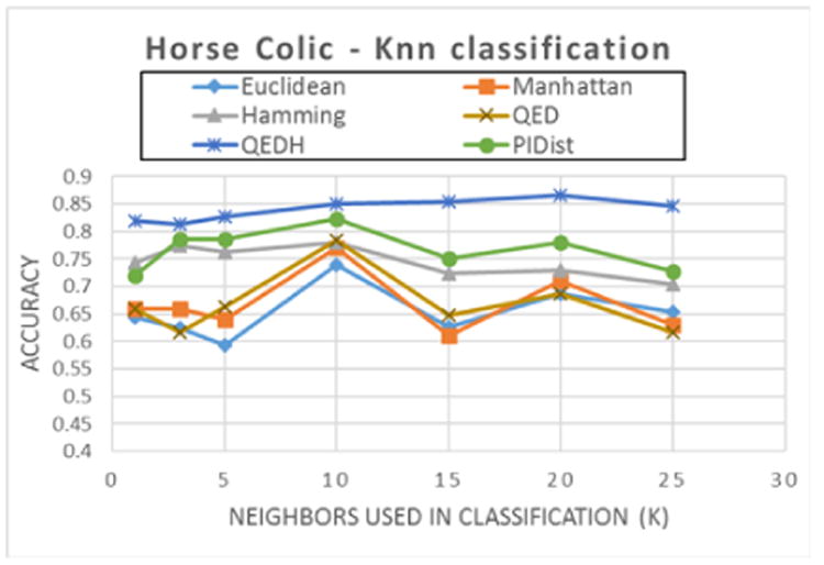
Figure 4. kNN Classification accuracy as the number of nearest neighbors (k) increases for Arrhythmia dataset. (Dataset: Arrhythmia, 452 rows, 279 attributes, 13 classes).

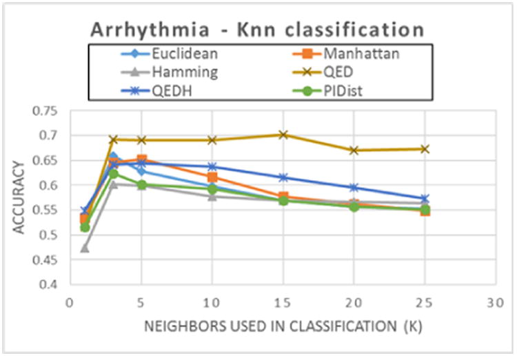
For the Arrhythmia dataset, figure 4, QED (with Manhattan distance) has the highest accuracy. It is worth noting that while the accuracy performance for other distance functions decreases as k increases, classification accuracy for QED is not significantly affected.

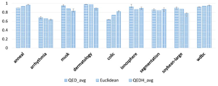
Figure 5 shows the average k-NN classification accuracy when varying p, the number of data points considered for QED. We vary p = {60%, 50%, 40%, 30%, 25%, 20%, 10%, 5%, and 1%}. The value of K was set to 5 for this figure. The error bar in each column shows the maximum and minimum measured accuracy. As shown, the performance of QED, while dependent on p is robust for different values of p. Furthermore, at least one QED approaches has a higher average accuracy than euclidean for each dataset.

Figure 5. kNN Classification accuracy by dataset with varying the range for p: 1% < p < 60% (the error bars show the maximum and minimum accuracy as p varies). k was set to 5.

4.3 QED for clustering

For this experiment we illustrate QED as a suitable quantization for high-dimensional data clustering. For this experiment, we sorted the data points using the class label, computed the distance between each pair of points, and plotted the distance matrix as a heat-map. A black pixel represents a distance of 0. Figure 6 shows the distance matrix heat-map for the Ionosphere dataset. This dataset has two classes which can be clearly seen in Figure 6d QED in the form of two darker squares along the diagonal, while in Figures 6a, 6b, and 6c, one of the classes is not clearly distinguishable. We observed similar results for some of the other datasets described in Table 1 but omitted them for space constraints.

Figure 6. The heatmap of the distance matrix for the Ionosphere dataset computed with a) Manhattan distance, b) Euclidean distance, c) Hamming distance, and d) QED.

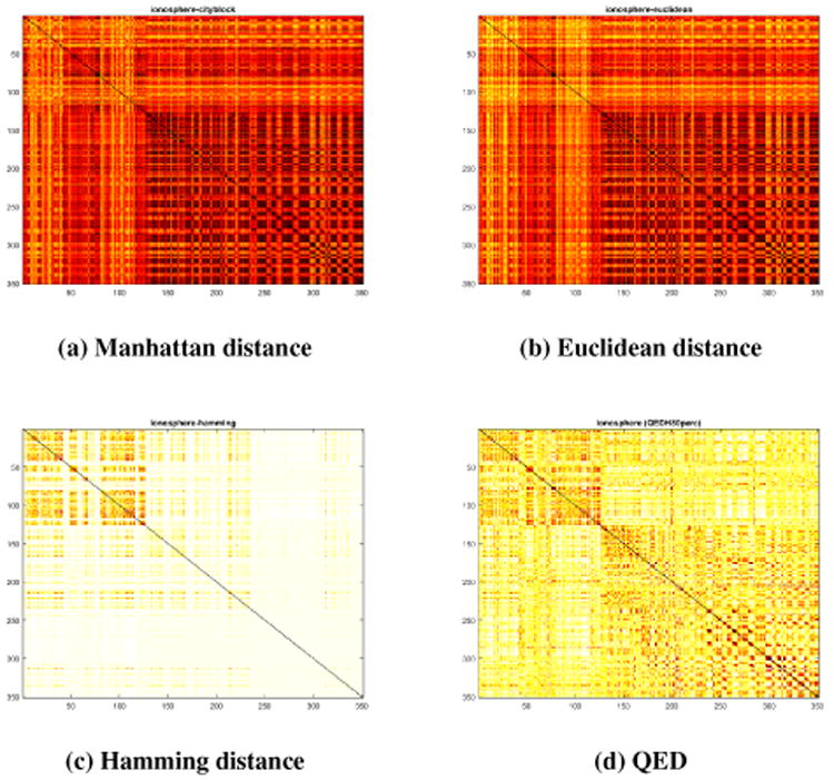
Many popular clustering algorithms use distance matrices to decide what points to cluster together. This experiment suggests that using QED instead of more traditional distance metrics could improve clustering accuracy.

5 Conclusion

In this work we described how bit-sliced indexing can be used to support k-Nearest Neighbor queries over high-dimensional data and efficiently perform on-the-fly Query dependent Equi-Depth (QED) quantization to improve the accuracy of the results. The quantization is done for each dimension at query time and localized scores are generated for the closest x% of the points with a constant penalty for the rest of the points.

We evaluated the kNN classification accuracy of the proposed QED quantization on a set of nine high-dimensional datasets and observed an average improvement in accuracy of 2.4% for Manhattan distance and 10.95% for Hamming distance when using QED quantization. We also showed that the proposed quantization makes the classification accuracy more robust to increasing number of neighbors which makes it suitable for clustering algorithms.

The BSI structures used in this paper and the query algorithms used as building blocks to support the kNN searches are designed for distributed processing. In future work, we want to evaluate the scalability as the dimensionality increases using a Spark/Hadoop cluster. We also need to evaluate the effect of QED quantization over query time.

References

- 1.Acker James G, Gregory Leptoukh. Online analysis enhances use of NASA earth science data. Eos, Transactions American Geophysical Union 88. 2007;2(2007):14–17. [Google Scholar]
- 2.Aggarwal Charu C, Yu Philip S. Proceedings of the sixth ACM SIGKDD international conference on Knowledge discovery and data mining. ACM; 2000. The IGrid index: reversing the dimensionality curse for similarity indexing in high dimensional space; pp. 119–129. [Google Scholar]
- 3.Beyer Kevin, Goldstein Jonathan, Ramakrishnan Raghu, Shaft Uri. International conference on database theory. Springer; 1999. When is “nearest neighbor” meaningful? pp. 217–235. [Google Scholar]
- 4.Blake C, Merz CJ. Department of Information and Computer Science. University of California; Irvine, CA: 1998. UCI repository of machine learning databases. [ http://www.ics.uci.edu/mlearn/MLRepository.html] 1998. [Google Scholar]
- 5.Donoho David L, et al. High-dimensional data analysis: The curses and blessings of dimensionality. AMS Math Challenges Lecture. 2000;1(2000):32. [Google Scholar]
- 6.García Salvador, Luengo Julián, Antonio Sáez José, López Victoria, Herrera Francisco. A Survey of Discretization Techniques: Taxonomy and Empirical Analysis in Supervised Learnings. IEEE Trans Knowl Data Eng 25. 2013;4(2013):734–750. [Google Scholar]
- 7.Guzun Gheorghi, Canahuate Guadalupe. Hybrid query optimization for hard-to-compress bit-vectors. The VLDB Journal (2015) 2015:1–16. [Google Scholar]
- 8.Guzun Gheorghi, Canahuate Guadalupe, Chiu David. A Two-Phase MapReduce Algorithm for Scalable Preference Queries over High-Dimensional Data. Proceedings of the 20th International Database Engineering & Applications Symposium (IDEAS) 2016 [Google Scholar]
- 9.Guzun Gheorghi, Tosado Joel, Canahuate Guadalupe. Transactions on Large-Scale Data-and Knowledge-Centered Systems XIV. Springer; 2014. Slicing the Dimensionality: Top-k Query Processing for High-Dimensional Spaces; pp. 26–50. [Google Scholar]
- 10.Indyk Piotr, Motwani Rajeev. Proceedings of the thirtieth annual ACM symposium on Theory of computing. ACM; 1998. Approximate nearest neighbors: towards removing the curse of dimensionality; pp. 604–613. [Google Scholar]
- 11.O'Neil PE, Quass D. Proceedings of the 1997 ACM SIGMOD international conference on Management of data. ACM Press; 1997. Improved query performance with variant indexes; pp. 38–49. [Google Scholar]
- 12.Rinfret Denis. Proceedings of the 2008 C 3 S 2 E conference. ACM; 2008. Answering preference queries with bit-sliced index arithmetic; pp. 173–185. [Google Scholar]
- 13.Rinfret Denis, O'Neil Patrick, O'Neil Elizabeth. Bit-sliced index arithmetic. ACM SIGMOD Record. 2001;30:47–57. ACM. [Google Scholar]
- 14.Goh King shy, Li Beitao, Chang Edward. DynDex: A Dynamic and Non-metric Space Indexer. ACM MULTIMEDIA. 2002:466–475. [Google Scholar]
- 15.Anthony K, Tung H, Rui Zhang, Nick Koudas, Ooi Beng Chin. VLDB'2006: Proceedings of the 32nd international conference on Very large data bases. VLDB Endowment; 2006. Similarity search: a matching based approach; pp. 631–642. [Google Scholar]