HUMAN DECISIONS AND MACHINE PREDICTIONS

Abstract

Can machine learning improve human decision making? Bail decisions provide a good test case. Millions of times each year, judges make jail-or-release decisions that hinge on a prediction of what a defendant would do if released. The concreteness of the prediction task combined with the volume of data available makes this a promising machine-learning application. Yet comparing the algorithm to judges proves complicated. First, the available data are generated by prior judge decisions. We only observe crime outcomes for released defendants, not for those judges detained. This makes it hard to evaluate counterfactual decision rules based on algorithmic predictions. Second, judges may have a broader set of preferences than the variable the algorithm predicts; for instance, judges may care specifically about violent crimes or about racial inequities. We deal with these problems using different econometric strategies, such as quasi-random assignment of cases to judges. Even accounting for these concerns, our results suggest potentially large welfare gains: one policy simulation shows crime reductions up to 24.7% with no change in jailing rates, or jailing rate reductions up to 41.9% with no increase in crime rates. Moreover, all categories of crime, including violent crimes, show reductions; and these gains can be achieved while simultaneously reducing racial disparities. These results suggest that while machine learning can be valuable, realizing this value requires integrating these tools into an economic framework: being clear about the link between predictions and decisions; specifying the scope of payoff functions; and constructing unbiased decision counterfactuals. JEL Codes: C10 (Econometric and statistical methods and methodology), C55 (Large datasets: Modeling and analysis), K40 (Legal procedure, the legal system, and illegal behavior)

I. INTRODUCTION

Many important decisions hinge on a prediction: managers assess future productivity for hiring; lenders forecast repayment; doctors form diagnostic and prognostic estimates; even economics PhD admissions committees assess future success (Athey et al., 2007; Chalfin et al., 2016). These predictions can be imperfect since they may rely on limited experience and faulty mental models and probabilistic reasoning. Could we use statistically-driven predictions to improve decision making in these prediction policy problems (Kleinberg et al., 2015)? This question, with old roots in psychology and criminology (Ohlin and Duncan, 1949, Meehl, 1954, Dawes, Faust, and Meehl, 1989), has renewed relevance today. Not only can large volumes of data now be brought to bear on many decisions, we also have new computational tools for analyzing these data. In particular, machine learning represents a pragmatic breakthrough in making predictions, by finding complex structures and patterns in data.¹ These developments make building and implementing decision aids an increasingly realistic possibility. We study one example, significant in its own right, to both understand the promise of using machine learning to improve decision making as well as reveal the unique (and often ignored) challenges that arise.

Each year in the United States, the police arrest over 10 million people (FBI, 2016). Soon after arrest, a judge decides where defendants will await trial, at home or in jail. By law, this decision should be based solely on a prediction: What will the defendant do if released? Will they flee or commit a new crime? A judge must trade off these risks against the cost of incarceration. This is a consequential decision for defendants since jail spells typically last several months (or longer); recent research documents large costs of detention even over the long term.² It is also costly to society: at any point in time the US has over 750,000 people in jail, disproportionately drawn from disadvantaged and minority populations (Henrichson, Renaldi, and Delaney, 2015). Currently the predictions on which these decisions are based are, in most jurisdictions, formed by some judge processing available case information in their head.

In principle an algorithm could also make these predictions. Just as pixel patterns can be used to predict presence of a face, information about the defendant and their case could be used to predict flight or public safety risk. We build such an algorithm–specifically, gradient boosted decision trees (Friedman 2001) using a large dataset of cases heard in New York City from 2008 to 2013. The algorithm uses as inputs only data available to the judges at the time of the bail hearing (e.g. current offense, prior criminal history); it does not use race, ethnicity or gender. Because New York state law requires judges to only consider flight risk when making pretrial release decisions, we initially train our algorithm on this outcome. Since we demonstrate below that our results also hold for other crime outcomes, including re-arrest, for convenience we refer to our outcome generically as ‘crime.’

The central challenge we face is not so much in building the algorithm, but rather in assessing whether its predictions actually improve on judges’ decisions. One of the core problems stems from missing data: we do not observe whether jailed defendants would have committed crimes had they been released. This problem is aggravated by the fact that judges surely rely on many factors that are unmeasured in our data. If judges observe, say, gang membership and only release teenagers not in gangs, then released youth may have different crime risks than jailed ones. If unaddressed, this could bias any comparison between judge and algorithm in favor of the algorithm.

To overcome this problem we rely in part on the fact that it is one-sided: counterfactuals in which the algorithm jails additional defendants can be readily evaluated. The problem only arises with counterfactuals where the algorithm releases defendants that judges would not. We also exploit the fact that in our data, defendants are as-good-as-randomly assigned to judges who differ in leniency.³ This allows us to combine the decisions of more lenient judges with the algorithm’s predictions and compare the results against the decisions of more stringent judges. We develop a simple framework that clarifies what assumptions are needed about judges’ preferences and release rules in order to construct these benchmarks. In all cases we can make meaningful comparisons without imposing specific preferences on how society or judges trade off crime versus jailing rates.

Three types of results together suggest algorithmic predictions can indeed improve judicial decisions. First, judges are releasing many defendants the algorithm ex ante identifies as very high risk. For example the riskiest 1% of defendants, when released, fail to appear for court at a 56.3% rate and are re-arrested at a 62.7% rate. Yet judges release 48.5% of them. Second, stricter judges do not jail the riskiest defendants first; instead they appear to draw additional detainees from throughout the predicted risk distribution. If additional defendants were selected instead according to predicted risk, stricter judges could produce outcomes that appear to dominate their current decisions: They could jail 48.2% as many people with the same reduction in crime, or for the same detention rate, they could have a 75.8% larger crime reduction.⁴ Third, we calculate bounds on the performance of an algorithmic release rule that reranks all cases by predicted risk, including a worst-case bound tantamount to assuming all jailed defendants are sure to commit crime. We show how random assignment of cases to judges is central to the calculation of these bounds. The algorithmic rule, at the same jailing rate as the judges, could reduce crime by no less than 14.4% and up to 24.7%; or without any increase in crime, the algorithmic rule could reduce jail rates by no less than 18.5% and up to 41.9%.⁵ These results are not unique to New York City; we obtain qualitatively similar findings in a national dataset as well.

These results, which focus on crime, could be misleading if the algorithm’s crime reductions are coming at the expense of other goals the judge (or society) values. For example one such goal is racial equity. Though we do not use race as an explicit input in prediction, other variables might be correlated with race. The algorithm could in principle reduce crime but aggravate racial disparities. Yet the opposite appears to be true in our data: a properly built algorithm can reduce crime and jail populations while simultaneously reducing racial disparities. In this case, the algorithm can be a force for racial equity. Similar problems may arise if judges weigh different kinds of crimes differently (for example prioritize risk of violent crime), or view detention of some defendants (such as those with jobs or families) as particularly costly. We present evidence that the algorithm’s release rule does no worse than the judges (and typically much better) on each outcome. Though we can never be certain of the full breadth of judicial preferences, these findings combined with the law’s injunction to focus solely on defendant risk suggest that algorithmic predictions likely can improve on judges’ decisions.

Machine learning could also be used to diagnose why judges mispredict. As a behavioral diagnostic, we build another algorithm that predicts judges’ release decisions. Both the predictable and unpredictable parts of judicial behavior prove revealing. We find for example that judges struggle most with high-risk cases: the variability in predicted release probabilities is much higher for high- than low-risk cases. In addition the judges’ decisions are too noisy. When judge decisions vary from our predictions of their decisions, the result is worse outcomes: a release rule based on the predicted judge dominates the actual judges’ decisions.⁶ These deviations from predicted behavior were, presumably, due to unobserved factors the judge sees but are not captured in our data. Economists typically focus on how these variables reflect private information and so should improve decisions. Psychologists, on the other hand, focus on how inconsistency across choices can reflect noise and worsens decisions (Kahneman et al., 2016). While we cannot separately quantify these two effects, the superior performance of the predicted judge suggests that, on net, the costs of inconsistency outweigh the gains from private information in our context. Whether these unobserved variables are internal states, such as mood, or specific features of the case that are salient and overweighted, such as the defendant’s appearance, the net result is to create noise, not signal.⁷

More generally the bail application provides a template for when and how machine learning might be used to improve on human decisions. First, it illustrates the kind of decisions that make for an ideal application of machine learning: ones that hinge on the prediction of some outcome (Kleinberg et al., 2015). Many applied empirical papers focus on informing decisions where the key unknown is a causal relationship; for example, the decision to expand college scholarship eligibility depends on the causal effect of the scholarship. The causal effect of jail on flight or public safety risk, though, is known. What is unknown is the risk itself. The bail decision relies on machine learning’s unique strengths (maximize prediction quality) while avoiding its weaknesses (not guaranteeing causal, or even consistent, estimates).⁸

A second general lesson is that assessing whether machine predictions improve on human decisions requires confronting a basic selection problem: data on outcomes (labels) can be missing in a nonrandom way. This problem is generic: very often the decisions of the human to whom we are comparing our algorithm generate the data we have available.⁹ As we have seen, this selective labels problem complicates our ability to compare human judgments and machine predictions. Solving this problem requires recognizing that decision makers might use unobserved variables in making their decision: one cannot simply use observable characteristics to adjust for this selection.

A final lesson is the need to account for the decision maker’s full payoff function: decisions that appear bad may simply reflect different goals. In causal inference, biases arise when omitted variables correlate with the outcome. But for prediction, biases arise when omitted variables correlate with payoffs. Predictions based on only one of the variables that enter the payoff function can lead to faulty conclusions. We chose bail explicitly because the potential for omitted-payoff biases are specific and narrow in scope. Yet even here concerns arose. We worried, for example, that our improved performance on crime was being undermined by creating racial inequity. The problem is put into sharp relief by considering a different decision that initially seems similar to bail: sentencing. Recidivism, which is one relevant input to sentencing someone who has been found guilty, can be predicted. Yet many other factors enter this decision—deterrence, retribution, remorse—which are not even measured. In many other applications, such biases could loom even larger. For example, colleges admitting students, police deciding where to patrol, or firms hiring employees all maximize a complex set of preferences (Chalfin et al., 2016). Outperforming the decision maker on the single dimension we predict need not imply the decision maker is mispredicting, or that we can improve their decisions.

It is telling that in our application, much of the work happens after the prediction function was estimated. Most of our effort went to dealing with selective labels and omitted payoffs, towards synthesizing machine-learning techniques with more traditional methods in the applied economics toolkit. Even for social science applications such as this, where the key decision of concern clearly hinges on a prediction, better algorithms alone are of ambiguous value. They only become useful when their role in decision making is made clear, and we can construct precise counterfactuals whose welfare gains can be calculated.

These challenges are largely overlooked in the existing literature. Dating back to at least the 1930s social scientists have tried to predict criminal behavior, although typically without any direct attempt to establish performance relative to a human’s decision.¹⁰ Some recent papers in computer science, though, acknowledge the selective labels problem and seek to address it in the bail context using carefully designed methods to impute outcomes for defendants who are missing labels (Lakkaraju and Rudin, 2016, and Jung et al. 2017). For example, Lakkaraju and Rudin (2016) employ doubly-robust estimation that combines inverse propensity-score weighting and logistic regression, while Jung et al. (2017) use a regularized logistic regression model. These methods all rely on a ‘selection on observables’ assumption to impute outcomes.¹¹ But assuming away the role of unobservables removes a key source of potential judicial advantage and as a consequence biases results in favor of the algorithm. Existing work has also been less sensitive to omitted-payoff bias, focusing on individual outcomes rather than on the full payoffs surrounding a decision; in bail, for example, only examining outcomes like FTA.¹²

These same challenges are relevant for the older, foundational efforts within psychology to compare human predictions to statistical rules (e.g. Meehl, 1954, Dawes, 1971, 1979, Dawes, Faust and Meehl, 1989, and Grove et al., 2000). They largely ignored selective labels and, to a lesser degree, also ignored omitted-payoff biases, and to the extent to which these issues were noted they were not resolved.¹³ While this earlier work proved visionary, given these potential biases it is hard to interpret the resulting statistical evidence. If the ultimate goal is to meaningfully compare human decisions to machine predictions, it would be unfair to ignore these factors. By assuming away humans’ potential for private information or for richer payoffs in making the decisions they do, the result is biased towards the conclusion of algorithms being better.

II. DATA AND CONTEXT

II.A. Pretrial bail decisions

Shortly after arrest, defendants appear at a bail hearing. In general judges can decide to release the defendant outright (such as to release on recognizance, or ROR), set a dollar bail that must be posted to go free, or detain the defendant outright.¹⁴ As noted above, these hearings are not intended to determine if the person is guilty, or what the appropriate punishment is for the alleged offense. Judges are asked instead to carry out a narrowly defined task: decide where the defendant will spend the pretrial period based on a prediction of whether the defendant, if released, would fail to appear in court (‘FTA’) or be re-arrested for a new crime.

When judges set money bail, they technically make two predictions - crime risk, and the ability to pay different bail amounts.¹⁵ Our decision, for simplicity, to treat these as a single compound decision could affect our findings in several ways. Judges may be making mistakes in predicting either crime risk or ability to pay, which may complicate our ability to isolate misprediction of risk. At the same time, forcing the algorithm to make a single decision narrows its choice set, which on the surface should limit its performance relative to a broader space of available choices. Below we show our results are not sensitive to how we handle this.

When making these decisions, judges know the current offenses for which the person was arrested and the defendant’s prior criminal record (‘rap sheet’). In some places, pretrial services will interview defendants about things that may be relevant for risk, such as employment status or living circumstances. Of course the judge also sees the defendants, including their demeanor and what they are wearing (which is typically what they wore at arrest), and whether family or friends showed up in court.

The context for most of our analysis is New York City, which has the advantages of providing large numbers of observations and was able to provide data that identifies which cases were heard by the same judges. Yet the pretrial system in New York is somewhat different from other places. First, New York is one of a handful of states that asks judges to only consider flight risk, not public safety risk.¹⁶ So we focus our models for New York initially on FTA, although we also explore below what happens when we consider other outcomes. Second, in New York many arrestees never have a pretrial release hearing because either the police give them a desk appearance ticket, or the case is dismissed or otherwise disposed of in bond court. So we drop these cases from our analysis. Third, judges in New York are given a release recommendation based on a six-item checklist developed by a local nonprofit, so our analysis technically compares the performance of our algorithm against the combined performance of the judges plus whatever signal they take from this existing checklist tool.¹⁷ To determine how important these local features are we also replicate our analysis in a national dataset as well, discussed in Online Appendix A.

II.B. Data

We have data on all arrests made in New York City between November 1, 2008 and November 1, 2013. The original data file includes information about 1,460,462 cases. These data include much of the information available to the judge at the time of the bail hearing, such as current offense, rap sheet, and prior FTAs.¹⁸ The dataset also includes the outcome of each case, including whether the defendant was released, failed to appear in court (FTA), or was re-arrested prior to resolution of the case.¹⁹ The only measure of defendant demographics we use to train the algorithm is age.²⁰

Of the initial sample, 758,027 were subject to a pretrial release decision and so are relevant for our analysis.²¹ Since our goal is accurate out-of-sample prediction, we divide the data into a training data set that the algorithm is fitted on and we then use the remaining data, a ‘test’ or ‘hold out’ set, to evaluate the algorithm. This prevents the algorithm from appearing to do well simply because it is being evaluated on data that it has already seen. As an extra layer of protection, to ensure that our results are not an artifact of unhelpful ‘human data mining,’ as shown in Figure I we follow Tan, Lee, and Pang (2014) and also form a ‘pure hold-out’ of 203,338 cases. This final hold-out set was constructed by randomly sampling some judges and taking all of their cases, selecting a random selection of cases from the remaining judges, and also selecting the last 6 months of the data period. We have not touched this dataset until production of this final draft of our manuscript; below we show that our main results replicate in this new test set. This leaves us with a main working dataset of 554,689 cases, which we randomly partition into 40% training, 40% imputation and 20% test data sets. Unless otherwise noted, the predictive algorithms used to generate the exhibits are trained on the 221,876 observation training set, and then evaluated on the 110,938 observation hold-out set. For now we focus on the training and test sets, and later in the paper we return to the role of the remaining 40% imputation set. Figure I provides a schematic representation of these basic elements.

Figure I. Partition of New York City Data (2008–13) into Data Sets Used for Prediction and Evaluation.

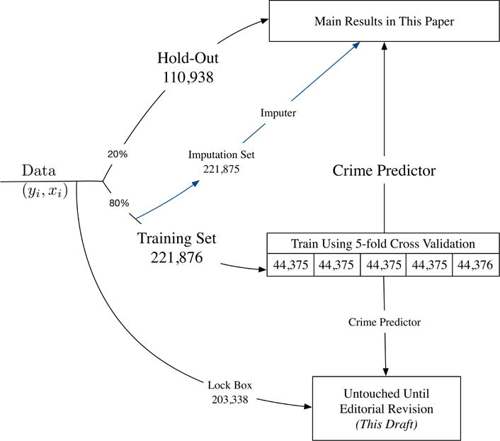
Notes: We show here the partitioning and analysis strategy for our dataset from New York City covering arrests from November 1, 2008 through November 1, 2013. The original sample size is 1,460,462. For our analysis we drop cases that were not subject to a pretrial release hearing, which leaves us with a total of 758,027 observations. We selected the final hold-out set of 203,338 by taking all cases arraigned in the last six months of our dataset (all cases arraigned after May 1, 2013), randomly selecting all cases heard by judges among the 25 judges with the largest caseloads until reaching 10% of total observations, which winds up selecting 7 judges, and randomly selecting 10% of all observations (these samples can be overlapping). In this draft we evaluate all of our results by randomly selecting a test set of 20% of the remaining 556,842 observations in our working sample. The remaining data is evenly divided between a training set that is used to form the algorithmic crime predictions used in all our analysis; and an imputation set used to impute crime risk (when needed) for jailed defendants. To account for potential human data-mining, this lock box set was untouched until the revision stage (this draft): in Table A.8 we replicate key findings on this previously untouched sample.

Table I presents descriptive statistics for our analysis sample. As is true in the criminal justice systems of many American cities, males (83.2%) and minorities (48.8% African-American, 33.3% Hispanic) are overrepresented. A total of 36.2% of our sample was arrested for some sort of violent crime, 17.1% for property crimes, 25.5% for drug crimes, and the rest a mix of various offenses like driving under the influence, weapons, and prostitution. Overall 73.6% of defendants were released prior to adjudication, which includes everyone released on recognizance (63.2% of all defendants), plus about a third of those offered bail (35.5%). Those we call ‘detained by the judge’ includes the two-thirds of those offered bail who cannot make bail, plus the 1.3% of defendants who are remanded (denied bail). We initially do not distinguish between the chance to post bail versus being assigned high bail, though we return to this below.

Table I.

Summary Statistics for New York City Data, 2008–13

	Full Sample	Judge Releases	Judge Detains	p-value
Sample Size	554,689	408,283	146,406
Release Rate	0.7361	1.0000	0.00
Outcomes
Failure to Appear (FTA)	0.1112	0.1521
Arrest (NCA)	0.1900	0.2581
Violent Crime (NVCA)	0.0274	0.0372
Murder, Rape, Robbery (NMRR)	0.0138	0.0187
Defendant Characteristics
Age	31.98	31.32	33.84	<.0001
Male	0.8315	0.8086	0.8955	<.0001
White	0.1273	0.1407	0.0897	<.0001
African American	0.4884	0.4578	0.5737	<.0001
Hispanic	0.3327	0.3383	0.3172	<.0001
Arrest County
Brooklyn	0.2901	0.2889	0.2937	.0006
Bronx	0.2221	0.2172	0.2356	<.0001
Manhattan	0.2507	0.2398	0.2813	<.0001
Queens	0.1927	0.2067	0.1535	<.0001
Staten Island	0.0440	0.0471	0.0356	<.0001
Arrest Charge
Violent Crime
Violent Felony	0.1478	0.1193	0.2272	<.0001
Murder, Rape, Robbery	0.0581	0.0391	0.1110	<.0001
Aggravated Assault	0.0853	0.0867	0.0812	<.0001
Simple Assault	0.2144	0.2434	0.1335	<.0001
Property Crime
Burglary	0.0206	0.0125	0.0433	<.0001
Larceny	0.0738	0.0659	0.0959	<.0001
MV Theft	0.0067	0.0060	0.0087	<.0001
Arson	0.0006	0.0003	0.0014	<.0001
Fraud	0.0696	0.0763	0.0507	<.0001
Other Crime
Weapons	0.0515	0.0502	0.0552	<.0001
Sex Offenses	0.0089	0.0086	0.0096	.0009
Prostitution	0.0139	0.0161	0.0078	<.0001
DUI	0.0475	0.0615	0.0084	<.0001
Other	0.1375	0.1433	0.1216	<.0001
Gun Charge	0.0335	0.0213	0.0674	<.0001
Drug Crime
Drug Felony	0.1411	0.1175	0.2067	<.0001
Drug Misdemeanor	0.1142	0.1156	0.1105	<.0001
Defendant Priors
FTAs	2.093	1.305	4.288	<.0001
Felony Arrests	3.177	2.119	6.127	<.0001
Felony Convictions	0.6157	0.3879	1.251	<.0001
Misdemeanor Arrests	5.119	3.349	10.06	<.0001
Misdemeanor Convictions	3.122	1.562	7.473	<.0001
Violent Felony Arrests	1.017	0.7084	1.879	<.0001
Violent Felony Convictions	0.1521	0.1007	0.2955	<.0001
Drug Arrests	3.205	2.144	6.163	<.0001
Felony Drug Convictions	0.2741	0.1778	0.5429	<.0001
Misdemeanor Drug Convictions	1.049	0.5408	2.465	<.0001
Gun Arrests	0.2194	0.1678	0.3632	<.0001
Gun Convictions	0.0462	0.0362	0.0741	<.0001

Notes: This table shows descriptive statistics overall and by judge release decision for the 554,689 cases that serve as our New York City analysis dataset shown in Figure I. For each variable, we perform a test of the equality of means between released and detained defendants. Released defendants are defined as those who are released outright by judges, as well as those assigned cash bail who are released because they make bail. Detained defendants are those who are assigned cash bail and cannot make bail, together with those who are remanded (no offered bail). Failure to appear is defined as not showing up at a required court hearing prior to adjudication of the defendant’s case, as measured from court records. Re-arrest is defined as being arrested again prior to adjudication of the case; this could include some defendants who are arrested as a result of a failure to appear. The p-value for this test are in the last column.

Among released defendants 15.2% fail to appear (FTA) at a subsequent court hearing prior to adjudication of their case, as indicated by court records. In addition 25.8% are re-arrested prior to adjudication; a small share of these arrests may be related to arrest warrants issued in response to a FTA.²² Among the released, 3.7% are arrested for a violent crime specifically, and 1.9% for murder, rape, and robbery. We also show these outcomes for the full sample, where we use the value 0 for the jailed defendants. Tiny differences may appear in later Tables because some numbers below come from the 20% test set subsample.

Table I also makes clear that judges are paying some attention to defendant characteristics in deciding who to release, since the average values differ by release status. Exactly how good judges are in making these decisions relative to an algorithm’s predictions is the focus of the rest of our paper.

III. EMPIRICAL STRATEGY

Our empirical analysis essentially consists of two steps: train an algorithm, and then evaluate its performance. The first step will look quite similar to standard machine-learning practice: train an algorithm to produce a prediction function that relates defendant characteristics to an outcome such as failure to appear or re-arrest. In typical engineering applications like vision or language, the second evaluation step is straightforward: simply measure how well the fitted function predicts out of sample. However we are interested instead in what those predictions tell us about the quality of current human (judge) decisions, and whether using the algorithmic predictions can improve those decisions.

III.A. Forming the Prediction Function

We will take the outcome of interest Y to be an indicator for failure to appear, or FTA (or, when noted, an index of whether the defendant either FTA’s or is re-arrested), which we designate ‘crime.’ The input variables, X, consist of characteristics of the defendant’s current case, their prior criminal record, and age (but not other demographic features like race, ethnicity or gender). A key challenge is that we only observe Y for released defendants, which affects both training and evaluation of the algorithm.²³

We form predictions using gradient boosted decision trees (Friedman, 2001) to fit a function m(X) that outputs a predicted probability P (Y = 1|X) (though our results are similar with other algorithms). In a decision tree, the data is divided through a sequence of binary splits. For example, the first split might be whether the person has ever been arrested. In the next step we can split each of the two nodes created by that first split by different variables, allowing for a high degree of interactivity in our prediction function. At each final (‘leaf’) node, there is a value which is the prediction for every data point in that space. The gradient boosted trees algorithm is essentially an average of multiple decision trees that are built sequentially on the training data, with each subsequent iteration up-weighting the observations that have been predicted most poorly by the sequence of trees up to that point. The complexity of a gradient boosted tree model depends on the depth of each tree, the number of trees averaged together, and the weighting scheme for each subsequent tree. We select these parameters using five-fold cross-validation (see Figure I). Once the optimal model parameters are selected, we estimate the final model using the full training set.

A regression of the algorithm’s predicted values against a linear additive function of the baseline covariates yields an Adjusted R-squared of 0.51, which provides some initial indication that there is nonlinear structure in the data that machine-learning tools help identify. We show below that this additional nonlinear structure captures useful signal.²⁴

III.B. Evaluating the Prediction Function

Standard practice in machine learning would be to compare predicted probabilities m(X) to outcomes Y in the test data. A common metric for measuring prediction accuracy would be something like the area under the receiver operating characteristic curve (AUC), which in our case equals 0.707.²⁵ Measures such as these, though, do not tell us whether the algorithm’s predictions can improve on decision quality. For example, an algorithm that correctly identifies within the released set some defendants as having 0 risk and others as having 10% risk may do little to change decisions if society’s preference is to release even everyone with a 10% risk.

Evaluating whether m(X) can be used to improve judicial decisions raises its own challenges, which we illustrate using a simple framework. We take the prediction function as given, which in practical terms is what we would be doing when evaluating performance in a true holdout set. The framework must also specify the true underlying data-generating process. In our data, we have a binary Y variable and a multidimensional X about defendants. In the modeled data generating process, we assume Pr(Y = 1) = y, the defendant’s probability of committing a crime. Though the underlying data is multidimensional, we can model it as having only a few dimensions. Specifically, suppose in addition to X, judges observe (but we do not) a multidimensional Z. We could now define two unidimensional variables x(X) ≡ [Y |X] and z(X, Z) ≡ [Y |X, Z] −E[Y |X].

This motivates a model in which defendants are characterized by an observed x and an unobserved z (seen by the judge). In addition, we assume there are unobserved w (that captures something about the defendant or even the judge’s mental state) that affects the judge’s decision but does not have any information about y. This construction also motivates the assumption that:

$$E\left(y|X,Z\right)=E\left[y|x,z\right]=x+z$$

This assumption reflects the idea that while w might affect decisions, it does not predict risk. It also places some narrow restrictions such as that x and z are distributed so their sum is between 0 and 1, and assumes that the observed x is a single variable that (on average) equals risk. Finally, each case is heard by a judge j who makes a release decision R = 0, 1. We will assume that y; x; z and w are jointly distributed and all individuals are i.i.d. draws from this fixed distribution. Below we describe how R is determined. Additionally we assume there is a pool of judges who draw cases from the same distribution - in effect, random assignment of cases to judges.

We model judicial payoffs on a case by case basis, though for our purposes all that matters is that judges have an aggregate payoff function that is increasing in the release rate and decreasing in the crime rate. Each judge j has a payoff function π^j that depends on a defendant’s crime propensity and the release decision:

$${\pi }^i\left(y,R\right)=-\underset{\text{Crime Cost}}{\underbrace{a_{j}yR}}-\underset{\text{Incarceration Cost}}{\underbrace{b_j\left(1-R\right)}}$$

where a_j represents the weight the judge places on crimes committed and b_j the weight they place on incarcerating someone. Since crime is a binary outcome we can write the payoff function as linear in probability of crime.

We define ρ(x, z, w) to be a generic release rule (written as ρ for ease), and the expected payoff of this rule as ∏^j(ρ) = E[π^j(y; ρ)] where the expectation is taken over a randomly drawn y; x; w; z. Judge j then chooses an optimal release rule ρ^j that maximizes this expected payoff. Their rule depends on their (possibly erroneous) assessment of risk, which we write as h_j(x; z; w). Given this assessment, their release rule will be:

$${\rho }^j\left(x,z,w\right)=1\text{if and only if}{h}_j\left(x,z,w\right)<{\kappa }_j\equiv \frac{b_j}{a_j}$$

Defendants are released if their risk is below the judge’s threshold κ _j which is determined by how they weigh crimes committed (a_j) relative to incarceration costs (b_j).

The basic question we address is whether a given algorithm’s predictions m(x) can improve upon judicial predictions. In particular, we would like to evaluate whether there is a release rule d for judge j that combines their judgement h_j and m to produce a higher payoff for judge j, i.e. if ∏^j(ρ^d) >∏^j(ρ^j). Note that the difference between these two is:

$${\mathrm{\Pi }}^j\left({\rho }^d\right)-{\mathrm{\Pi }}^j\left({\rho }^j\right)=-a_j\underset{\mathrm{\Delta }\text{Crime}}{\underbrace{\left({\overline{R}}^{d}E\left[y|{\rho }^d=1\right]-{\overline{R}}^{j}E\left[y|{\rho }^j=1\right]\right)}}-b_j\underset{\mathrm{\Delta }\text{Release}}{\underbrace{{\overline{R}}^j-{\overline{R}}^d}}$$

where ${\overline{R}}^{\rho }$ denotes the release rate of any release rule and we write ${\overline{R}}^j$ as shorthand for ${\overline{R}}^{{\rho }^3}$. One challenge, to which we return below, is whether we know the preference parameters (a_j, b_j). If these were known, the effect of the second term can be calculated since the release rates are calculable. To abstract from this, for now, suppose we are considering an algorithmic release rule which makes the second term zero, i.e. where ${\overline{R}}^d={\overline{R}}^j$.

The remaining first term poses a more serious measurement problem. Since it cancels for cases where the judge and algorithm agree (i.e. if ρ^j = ρ^d), the difference is determined by the cases where they disagree; at ${\overline{R}}^d={\overline{R}}^j$ it is proportional to:

$$-\underset{\text{Measured}}{\underbrace{E\left[y|{\rho }^d=0,{\rho }^j=1\right]}}+\underset{\text{Unmeasured}}{\underbrace{E\left[y|{\rho }^d=1,{\rho }^j=0\right]}}$$

We can only measure the crime changes due to defendants released by the judge and jailed by the algorithm; but we cannot measure the changes due to the defendants jailed by the judge and released by the algorithm. Two points are worth noting here.

First, procedures in the literature typically use the observable data to resolve the lack of labels with, for example, propensity scores, imputation or Bayesian procedures. Even abstracting from estimation issues, at best these procedures amount to assuming crime rates of the jailed, E[y|ρ^j = 0; x], are equal to the crime rates of the released with similar x: E[y|ρ^j = 1, x]. The challenge, of course, is that

$$\underset{\text{Imputation Error at }x}{\underbrace{E\left[y|{\rho }^j=1,x\right]-E\left[y|{\rho }^j=0,x\right]}}=E\left[x+z|{\rho }^j=1,x\right]-E\left[x+z|{\rho }^j=0,x\right]=\left(E\left[x|{\rho }^j=1,x\right]-E\left[x|{\rho }^j=0,x\right]\right)+\left(E\left[z|{\rho }^j=1,x\right]-E\left[x|{\rho }^j=0,x\right]\right)=0+\underset{\text{Selective Release at}x}{\underbrace{E\left[z|{\rho }^j=1,x\right]-E\left[z|{\rho }^j=0,x\right]}}$$

If judges select at all on unobservables, there is no reason to believe that outcomes of the released with similar x serve as a good proxy of what the jailed would do if released. By ignoring unobserved factors, these imputation procedures have the potential to be very misleading. Consider a stylized example. Suppose that for young defendants, judges see gang tattoos and we do not, and that judges know this type of tattoo is highly predictive of crime risk so they never release anyone with a gang tattoo. The imputer would attribute to all young people the crime rate of those without gang tattoos. This could seriously understate the increase in crime that would result from a risk tool that released all young people. We refer to this as the selective labels problem - even for the exact same x, the defendants who have labels (i.e. the defendants judges released) need not be the same as the defendants who do not have labels.

Second, this problem is one-sided. We have no trouble calculating the other counterfactual, the effect of jailing defendants whom the judge releases (or what one might call contracting the released set). This evaluation problem is of course not unique to the bail context. It occurs in a variety of machine-learning applications whenever we are trying to compare the performance of an algorithm to human decisions using data generated by the human decision maker: for example using an algorithm to predict who should receive some medical test using data generated by previous doctor testing decisions. Both our solutions below to this problem rely on its one-sided nature.²⁶

IV. JUDGE DECISIONS AND MACHINE PREDICTIONS

IV.A. How risky are the riskiest people judges release?

To understand how we might exploit the one-sidedness of the selective labels problem, we begin by looking at the distribution of predictable risk among those defendants judges in fact release. (As a reminder, since judges in NYC are asked to predict only FTA risk, this is the outcome we predict in our models unless otherwise noted, although for convenience we refer to our outcome generically as ‘crime.’) The left panel of Figure II bins defendants in our test set into 1,000 equal-sized groups based on the predicted risk values from our algorithm, m(X_i) and plots the observed judge release rates against predicted risk.

Figure II. How Machine Predictions of Crime Risk Relate to Judge Release Decisions and Actual Crime Rates.

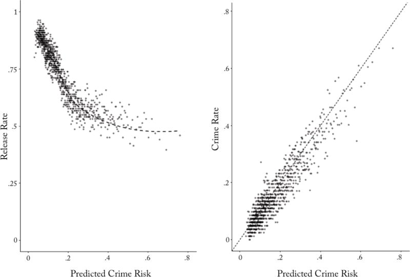
Notes: The figure shows the results of an algorithm built using 221,876 observations in our NYC training set, applied to the 110,938 observations in our test set (see Figure 1). Both panels show the algorithm’s predicted crime risk (defined here as predicted risk for failure to appear, or FTA) on the x-axis: each point represents one of 1,000 percentile bins. The left panel shows the release rate on the y-axis; the right panel shows the realized crime risk on the y-axis.

We see that at the low end of the predicted risk distribution, where most defendants are concentrated, judges release at a rate of over 90%. As predicted risk increases the judge release rate declines, which implies that the predictions of the judges and the algorithm are correlated. But we also see that the algorithm and the judges disagree, particularly at the high end of the risk distribution. If the predictions of the judges and the algorithm were identical, we would expect to see a step function: There would be some predicted-risk threshold where the release rate would be 0% above and 100% below. But that is not what we see. The curve relating judge release rates to the algorithm’s predicted crime risk flattens out as predicted risk increases. The riskiest 1% of defendants have a predicted risk of 62.6% yet are released at a 48.5% rate.²⁷

These release rates suggest a natural way to modify judicial decisions: jail those the judge releases but whom the algorithm predicts to be high risk. We define the release rule ρ^QC:

$$\text{Release if and only if}{\rho }^j=1\text{and}m\left(x\right)<{\kappa }_j$$

which contracts the release set by removing high risk defendants. We refer to this as quasi-contraction, in contrast to a more complete contraction procedure described below.

To understand whether this release rule can improve on judge’s payoffs, we calculate

$${\mathrm{\Pi }}^j\left({\rho }^{QC}\right)-{\mathrm{\Pi }}^j\left({\rho }^j\right)=P\left({\rho }^{QC}\ne {\rho }^j\right)\left(E\left[y^{QC}\ne {\rho }^j\right]-{\kappa }_j\right)$$

So the algorithm can improve upon decisions if it jails additional defendants (ρ^j = 1 & ρ^QC = 0) whose crime rates exceed the cost of incarceration (E[y] > κ_j).

The left panel of Figure II hints that there may be such defendants. But, of course the algorithm’s predictions are just predictions. In principle these defendants could actually be low risk, and the judges might realize this even if the algorithm does not. That is, perhaps the judges are able to identify defendants who look high risk with respect to the characteristics available to the algorithm, x, but are actually low risk with respect to features only the judges see, z.

Yet the right panel of Figure II shows that the people the algorithm predicts are risky are indeed risky. This figure relates observed crime rates to predicted risk, E[y|m(x)], among released defendants. This plot shows the data are clearly centered around the 45 degree line over almost all of the risk distribution. While this does not rule out the possibility that those defendants the judges detained versus released are different with respect to their unobservables (a point to which we return below), it does suggest that the defendants the judges released do not seem to have unusual unobservables that cause their observed outcomes to systematically diverge from what the algorithm had predicted. It also confirms that the defendants judges released who were predicted to be high risk are in fact high risk. For example, using just information the judge had at the time of the bail hearings, the defendants predicted to be riskiest by the machine-learning algorithm—the riskiest 1%—go on to have an observed crime rate of $\overline{Y}=56.3$.

As an aside, we can also explore the value added of machine learning relative to more familiar and simpler econometric methods for forming predictions. Table II compares the predicted risk distribution of the machine-learning algorithm to that produced by a logistic regression; specifically, we compare the cases flagged as risky by these two procedures.²⁸ At the 1^st percentile of the risk distribution (row 1), we see substantial disagreement in who is flagged as risky—only 30.6% of the cases flagged as top percentile in the predicted risk distribution by our machine-learning algorithm are also flagged as top percentile by the logistic regression (column 1). These defendants identified as high risk by both procedures also have the highest realized crime rates (60.8% in column 3). Those flagged only by the machine-learning algorithm are nearly as risky (54.4% in column 2), while those flagged only by the logit are far less risky (40% in column 3). As a result, algorithm-flagged defendants (column 4) are riskier as a whole than logit-flagged ones (column 5). This pattern repeats in the other rows but begins to attenuate the further we move down the predicted risk distribution (rows 2 through 4). By the time we reach the 25^th percentile of the distribution (row 4) the two procedures agree on 72.9% of the cases. As a whole, these results suggest that even in these data, which contain relatively few variables (compared to sample size), the machine-learning algorithm finds significant signal in combinations of variables that might otherwise be missed. These gains are most notable at the tail of the distribution and (somewhat predictably) attenuate as we move towards the center. This intuition suggests that were we to look at outcomes that have relatively lower prevalence (such as violent crimes, as we do in Section V.A.1.) the difference in results between the two prediction procedures would grow even starker.

Table II.

Comparing Logistic Regression to Machine-Learning Predictions of Crime Risk

Percentile Risk Percentile	ML/Logit Overlap	Average Observed Crime Rate for Cases Identified as High Risk by:
		Both ML & Logit	ML Only	Logit Only	All ML Cases	All Logit Cases
1%	30.6%	0.6080 (0.0309)	0.5440 (0.0209)	0.3996 (0.0206)	0.5636 (0.0173)	0.4633 (0.0174)
5%	59.9%	0.4826 (0.0101)	0.4090 (0.0121)	0.3040 (0.0114)	0.4531 (0.0078)	0.4111 (0.0077)
10%	65.9%	0.4134 (0.0067)	0.3466 (0.0090)	0.2532 (0.0082)	0.3907 (0.0054)	0.3589 (0.0053)
25%	72.9%	0.3271 (0.0038)	0.2445 (0.0058)	0.1608 (0.0049)	0.3048 (0.0032)	0.2821 (0.0031)

Notes: The table above shows the results of fitting a machine-learning (ML) algorithm or a logistic regression to our training dataset, to identify the highest-risk observations in our test set. Both machine-learning and logistic regression models are trained on the outcome of failure to appear (FTA). Each row presents statistics for the top part of the predicted risk distribution indicated in the first column: top 25% (N=20,423); 10% (8,173); 5% (4,087); and 1% (818). The second column shows the share of cases in the top X% of the predicted risk distribution that overlap between the set identified by ML and the set identified by logistic regression. The subsequent columns report the average crime rate observed among the released defendants within the top X% of the predicted risk distribution as identified by both ML and logit, ML only, and logit only, and all top X% identified by ML (whether or not they are also identified by logistic regression) and top X% identified by logit.

The key challenge with quasi-contraction is interpretational. We have established that the algorithm can ex ante identify defendants with a (56.3%) risk. By itself, this tells us that social gains are possible so long as society’s risk threshold for detention is below 56.3% – in this case, high risk defendants who should be jailed are being released. But it does not tell us that judges, by their own preferences, are mistaken: we do not know the risk threshold κ_j that they have. Without additional analysis, we cannot rule out the possibility that judges place such a high cost on jailing defendants that even this level of risk does not merit detention in their eyes.

IV.B. Using Differential Leniency

We overcome the challenge of not knowing κ_j by using the fact that judges have different release rates: crime rate differences between judges of different leniency provide benchmarks or bounds for how society currently trades off crime risk and detention costs. Forming such benchmarks requires some assumptions about the underlying data-generating process and how judges do, and do not, differ from one another.

The first assumption we will make is that judges draw from the same distribution of defendants. This assumption can be implemented in the NYC data by taking advantage of the fact that we have (anonymous) judge identifiers, together with the fact that conditional on borough, court house, year, month, and day of week, average defendant characteristics do not appear to be systematically related to judge leniency rates within these cells.²⁹ For this analysis we restrict our attention to the 577 cells that contain at least five judges (out of 1,628 total cells) in order to do comparisons across within-cell judge-leniency quintiles. These cells account for 56.5% of our total sample, with an average of 909 cases and 12.9 judges per cell. Online Appendix Table A.3 shows this sample is similar on average to the full sample. Online Appendix Table A.4 also shows that the stricter judges tend to be the ones who see fewer cases. This also implies a balance test must account for within-cell randomization and cannot simply compare mean defendant characteristics across judge leniency quintiles.

We carry out a permutation test that focuses on the projection of our outcome Y (in this case FTA) onto the baseline characteristics, which essentially creates an index of baseline defendant characteristics weighted in proportion to the strength of their relationship with the outcome. Separately for each borough, year, month and day of week cell, we regress this predicted value against a set of indicators for within-cell judge-leniency quintile, and calculate the F-test statistic for the null hypothesis that the judge leniency indicators are jointly zero. We then randomly permute the judge-leniency quintiles across cases M=1,000 times within each cell to form a distribution of F-test statistics calculated under the null hypothesis of no relationship between judge leniency and defendant characteristics. If defendant characteristics were systematically related to judge leniency, we would expect to see a concentration of our F-test statistics with low p-values. Yet Figure III shows that the histogram of p-values across the 577 cells in our analysis sample does not show unusual mass at low p-values. (See Online Appendix B for more details).

Figure III. Testing Quasi-Random Assignment of Defendants Across Leniency Quintiles Distribution of p-values for Balance Tests in Contraction Sample.

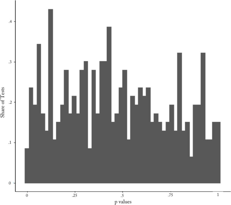
Notes: The figure shows the distribution of p-values for balance checks in our contraction sample summarized in Table A.3. We construct 577 borough, year, month and day of week ‘cells’ in the New York City data where we have at least five judges. We then define judge leniency quintiles within each cell. We regress each defendant’s predicted FTA (based on baseline characteristic) against dummies for leniency quintile and form anF-statistic for the test of the null that these dummies all equal zero; these are compared to a distribution of F-statistics produced by permuting the leniency quintile dummies randomly within each cell. The figure graphs the resulting p-value distribution. See Online Appendix A for more details.

The other thing we need for this design to work are differences in judge leniency within cells. As in past research, we see this in our data as well. The most lenient quintile judges release 82.9% of defendants. Relative to the most lenient judge quintile, less lenient quintiles have average release rates that are 6.6, 9.6, 13.5 and 22.3 percentage points lower, respectively.

Quasi-random assignment to judges together with differing leniency allow us to answer a straightforward question: if we begin with the most lenient judge’s caseload and detain additional defendants according to predicted risk, what crime and release rates are produced and how do these compare to what results from the decisions of more stringent judges? We discuss this below and will illustrate it in Figure V.

Figure V. Does Jailing Additional Defendants by Predicted Risk Improve on Judges? Contraction of the Most Lenient Judges’ Released Set.

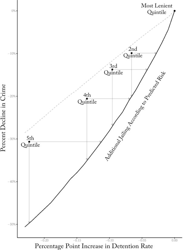
Notes: This figure looks at performance when additional defendants are jailed according to a predictive model of crime risk (defined here as predicted risk for failure to appear, or FTA), comparing crime rates and release rates to the actual decisions made by stricter judges. The rightmost point in the graph represents the release rate of the most lenient quintile of judges, with the crime rate that results. The solid line shows the crime reductions that we realize if we released defendants according to the predicted crime risk. By comparison, the light dashed line shows the decline in crime (as a percentage of the lenient quintile’s crime rate, shown on the y-axis) that results from randomly selecting additional defendants to detain from within the lenient quintile’s released cases, with the change in release rate relative to the lenient quintile shown on the x-axis. The four points on the graph show the crime rate / release rate outcomes that are observed for the actual decisions made by the second through fifth most lenient quintile judges, who see similar caseloads on average to those of the most lenient quintile judges.

However we are also interested in answering a second question: Can we build a decision aid for judges that improves their payoffs ∏^j? Answering this question requires making an additional assumption in our framework regarding judges’ ‘technologies.’ Each judge’s release rule depends on two factors: a preference κ_j between crimes and incarceration; and a ‘technology’ h_j for identifying riskiness of individuals. Since we will seek to use judges as benchmarks for each other, it is worth being precise about this distinction. In what follows, for simplicity, our framework focuses on the case of two judges, j = 1, 2 where judge 2 is more stringent than judge 1. Judge j, if asked to implement an arbitrary preference κ, could form the release rule:

$${\rho }^{j,\kappa }\left(x,z,w\right)=1\text{if and only if}{h}_j\left(x,z,w\right)<\kappa$$

Note that because any pair of judges have different technologies, there is no reason that ρ^1,κ = ρ^2,κ. We will assume that, while judges can have very different release rules, their ability to select on unobservables is the same. Specifically, when judge j (for some κ) releases a fraction l of all people with observed x, we can define their average unobservable quality to be ${\overline{z}}^j\left(x,l\right)$. Our assumption about similar capacity to select on unobservables can then be written as:

$$\left(\forall l,x\right):{\overline{z}}^1\left(x,l\right)={\overline{z}}^2\left(x,l\right)$$

Put in words, at different levels of leniency, in each x-cell, both judges would release people who on average have the same unobservables.

Of course, since we only observe each judge at a given level of leniency this cannot be tested directly. If we define ${\overline{R}}^j\left(x\right)$ as judge j’s lenience for individuals with observed x, we can empirically look at a weaker form of this assumption:

$${\overline{z}}_1\left(x,{\overline{R}}^1\left(x\right)\right)={\overline{z}}_2\left(x,{\overline{R}}^2\left(x\right)\right)$$

To test this, we train an algorithm on the released set of the most lenient quintile and then use that to impute crime rates to defendants released by the less lenient quintile judges. This in effect lets us test ${\overline{y}}^1\left(x,{\overline{R}}_1\left(x\right)\right)={\overline{y}}^2\left(x,{\overline{R}}^2\left(x\right)\right)$ which, given that x is the same, tests the difference in z. If the most lenient judges are better able to identify defendants with high-risk z than are the less lenient judges, the imputed values would be below the actual crime outcomes within the caseloads of the less lenient judges. Yet what we see is that within each of the stricter quintiles, the imputed and actual values are well calibrated across the full range of the risk distribution (as shown in the bottom four panels of Figure IV) - indeed not very different from plotting the predicted values calculated using the full training set against observed outcomes within the full training set (shown in the top panel of Figure IV). These results show no evidence that more lenient judges select differently on unobservables z within each x cell compared to the more stringent judges.³⁰ Of course, these results only tell us that imputed values are calibrated up to a point: they hold within the range of release rates we observe. For example, if in a particular x cell, every judge jails at least 10% of defendants, then those 10% could have arbitrary crime rates, far off from the imputed value, and we would never observe them.

Figure IV. Do Judges of Different Leniency Screen Differently on Unobservables? Evaluated Predictors Formed Using Most Lenient Quintile on Other Quintiles.

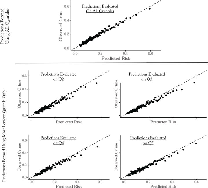
Notes: This figure tests whether the most lenient quintile judges in our NYC dataset are better at using ‘unobservables’ in making release / detain decisions than are the less lenient quintile judges. The top panel reproduces the calibration curve from Figure 2, plotting the algorithm’s predicted crime risk (defined here as predicted risk for failure to appear, or FTA) against observed crime rates within the test set. For the remaining panels, we train an algorithm using just the set of defendants released by the most lenient quintile judges, and then use that algorithm to generate predicted crime risk to compare to observed crime rates for the set of defendants released by the less lenient quintiles of judges.

With these assumptions in place, we can now form a meaningful test. Recall that judge 1 releases more people than judge $2:{\overline{R}}^1>{\overline{R}}^2$. We can therefore contract judge 1’s release set to produce a rule ρ^C:

$$\text{Release if and only if}{\rho }^1=1\text{and}m\left(x\right)<k$$

for some constant k. Because this rule releases only individuals released by judge 1 its crime performance is measurable:

$$E\left[y|{\rho }^C=1\right]=E\left[y|{\rho }^1=1,m\left(x\right)<k\right]$$

Relative to her own choices, this rule changes judge 2’s payoff by:

$${\mathrm{\Pi }}^2\left({\rho }^C\right)={\mathrm{\Pi }}^2\left({\rho }^2\right)=a_2\left(E\left[y|{\rho }^C=1\right]-E\left[y|{\rho }^2=1\right]\right)-b_2\left({\overline{R}}^2-{\overline{R}}^C\right)$$

As before, even without knowing the preference parameters, we can choose the constant k so that either we release the same number of defendants as judge 2 $\left({\overline{R}}^2-{\overline{R}}^C\right)$ or we achieve the same crime rate as judge 2 (E[Y¹|ρ^C = 1] = E[Y¹|ρ² = 1])). If we can achieve lower crime or higher release rates by doing this, then we will have improved outcomes given judge 2’s preferences irrespective of what her preferences are.

We can test this contraction procedure in our data. Starting with the released set of the most lenient judges, we can choose additional defendants to detain according to predicted risk. For each amount of additional incarceration, this allows us to calculate the crime rate that we observe for each of these (smaller) released sets. Importantly, because case characteristics are on average similar across judges, these numbers can be compared to the outcomes produced by the stricter judges. These results are presented graphically in Figure V. The solid curve calculates the crime that would have resulted if additional defendants had been detained in order of the algorithm’s predicted risk. Each of the points denotes the different judge leniency quintiles. Since any additional detention reduces crime for purely mechanical reasons (incapacitation), even randomly selecting defendants would reduce crime (the dashed line in the figure). The judge detention decisions are better than random, though one cannot tell whether they are doing much or only modestly better without a counterfactual.

When comparing each of the stricter judge quintiles to the algorithm, two points are particularly salient: (i) how much does crime fall when the algorithm increases jailing rates by the same amount; and (ii) what jailing increase does the algorithm need to achieve the same crime reduction as the judge?

The results presented in Table III show contraction produces significant gains over what judges manage. The second quintile of judges reduce crime by 9.9% relative to the most lenient quintile judges by increasing the detention rate by 6.6 percentage points. Our algorithm’s contraction curve shows that the same crime reduction could have been accomplished by increasing the detention rate by only 2.8 percentage points, or equivalently by increasing the detention rate by 6.6 percentage points we could have reduced crime by 20.1%. Put differently, relative to the observed judge outcomes we could have reduced the increase in jail population by only 42.1% as much, or increased the size of the crime drop by 103.0%. The magnitudes of these effects diminish somewhat as we move to the other leniency quintiles. Were we to average across all four of these quintiles we could jail only 48.2% as many people, or we could get crime reductions that are 75.8% larger.

Table III.

Does Jailing Additional Defendants by Predicted Risk Improve on Judges? Contraction of the Most Lenient Judges’ Released Set

	Judges		Algorithm
	Relative to Most Lenient Quintile		To Achieve Judge’s
			Δ Crime	Δ Jail
	Δ Jail	Δ Crime	Δ Jail	Δ Crime
Second Quintile	0.066	−0.099	0.028	−0.201
Third Quintile	0.096	−0.137	0.042	−0.269
Fourth Quintile	0.135	−0.206	0.068	−0.349
Fifth Quintile	0.223	−0.307	0.112	−0.498

Notes: This table reports the results of contrasting the cases detained by the second through fifth most lenient quintile judges compared with the most lenient quintile judges, and to a release rule that detains additional defendants in descending order of predicted risk from an algorithm trained on failure to appear. The first column shows from where in the predicted risk distribution each less lenient quintile’s judges could have drawn their marginal detainees to get from the most lenient quintile’s release rate down to their own release rate if judges were detaining in descending order of risk. The second column shows what share of their marginal detainees actually come from that part of the risk distribution. The fifth column shows the increase in the jail rate that would be required to reach each quintile’s reduction in crime rate if we jailed in descending order of the algorithm’s predicted risk, while the final column shows the reduction in crime that could be achieved if we increased the jail rate by as much as the judge quintile shown in that row.

This contraction rule could also form the basis for an implementable decision aid, though currently ρ^C improves judge 2’s payoffs by combining the algorithm with judge 1’s decisions, rather than with judge 2’s decisions. Under the assumptions we have made, though, ρ^C can also be implemented as a true decision aid: the algorithm combined with judge 2. By construction, there exist a set of x for which ρ^C jails everyone, call this X_C. For the remaining x, ρ^C releases at a rate equal to judge 1, so a release rate of ${\overline{R}}^1\left(x\right)$. A decision aid for judge 2 would therefore have that judge jail everyone with x in X_C, and then have them apply a leniency rate of ${\overline{R}}^1\left(x\right)$ for each x ∉ X_C. By construction, the crime rate for x ∈ X_C is 0, which also matches the crime rate of ρ^C in these cells. For x ∉ X_C, this produces a crime rate equal to $x+{\overline{z}}^2\left(x,{\overline{R}}^1\left(x\right)\right)$. By our assumption, however, this equals $x+{\overline{z}}^1\left(x,{\overline{R}}^1\left(x\right)\right)=E\left[y|{\rho }^C,x\right]$. The key reason we can turn ρ^C into an implementable decision aid is that we are assuming judges have similar technologies for selecting on unobservables, an assumption for which we provided supporting evidence above in Figure IV.

IV.C. Reranking

We have restricted our attention so far to two release rules that jail additional defendants relative to the judge. Both were carefully constructed to avoid the selective labels problem but neither captures the obvious release rule: release defendants solely based on the algorithm’s predicted risk; specifically, for some k, define the release rule

$${\rho }^m=1\text{if and only if}m\left(x\right)<k.$$

Evaluating the crime effects of this rule again raises the selective labels problem:

$$E\left[y|{\rho }^m=1\right]=P\left({\rho }^j=1\right)\underset{\text{Measured}}{\underbrace{E\left[y|{\rho }^j=1,{\rho }^m=1\right]}}+P\left({\rho }^j=0|{\rho }^m=1\right)\underset{\text{Unmeasured}}{\underbrace{E\left[y|{\rho }^j=0,{\rho }^m=1\right]}}$$

where j here denotes the judge a defendant was assigned to. To bound the extent of the selective labels problem, we would need to place a bound on the second term, the crime rate of the jailed. Since the algorithm’s release rule only depends on x, we can write this second term as $E\left[E\left[y|x,{\rho }^j=0\right]{\overline{R}}^{{\rho }^m}\left(x\right)\right]$. The central challenge of selective labels is how we calculate for each x the value E[y|x, ρ^j = 0]. Recall that:

$$E\left[y|{\rho }^j=0,x\right]=E\left[y|{\rho }^j=1,x\right]+\underset{\text{Selective Release at}x}{\underbrace{E\left[z|{\rho }^j=1,x\right]-E\left[z|{\rho }^j=0,x\right]}}$$

At one extreme, we could assume unobservables played no role so that the second term is zero: we would use the outcomes of the released as a proxy for the jailed. At the other extreme, notice that the unobservables could be arbitrarily large so that E[y|ρ^j = 0, x] = 1: everyone whom the judge jails is sure to commit a crime. This second extreme illustrates why, when we take seriously the possibility of judges using unobservable factors wisely, evaluating reranking is impossible without additional structure.

Two observations specific to bail provide structure that allows a tighter bound. The first is the quasi-random assignment of judges. Within each x cell, we have a variety of release rates by judge. Second, Figure IV show that the model is well calibrated even for the most lenient judges, suggesting unobservables play little role up to the release rate of the most lenient judges. So if, in a given x cell, the most lenient judge releases 80% of cases, we can assume up to 80% of defendants can be proxied for with E[y|x, ρ^j = 1]. Of course, the remaining 20% could have any crime rate.

In empirically evaluating any release rule, we use a bound derived from these observations. For those defendants for whom we have labels we use those labels.³¹ For the remaining defendants, up to the release rate of the most lenient judge in that x bin, ${\overline{R}}^l\left(x\right)$, we impute the label E[y|x, ρ^j = 1]. For the remainder we impute the label min{1, αE[y|x, ρ^j = 1]}, where α, the extent of the bound varies from 1 to ∞. Our imputed values come from fitting a separate set of gradient-boosted trees on the imputation set (the random 40% partition of our working dataset), which yields predictions of each defendant’s crime rate m(X_i). Results are similar if we use a logit imputer.

Because we would like a crime rate that can be meaningfully compared across release rates, we use the ratio of crimes committed by released defendants to the total number of defendants heard by the judge (not just the number released). In the Online Appendix, Figure A.2 graphs the crime rate (y-axis) that results at every possible target release rate (x-axis) when α = 1, the selection on observables assumption. To simplify the reranking analysis we initially assume that society’s preferences are reflected by the average choices of all the judges.

We find large potential gains if we assume no effect of unobservables: judges release 73.6% of defendants for a crime rate equal to 11.3% in the test set. At the judge’s release rate, the algorithm could reduce crime by 24.7%. Alternatively, at the judge’s crime rate, it can reduce the detention rate from 26.4% to 15.3%, for a decline of 41.9%. Translated into absolute numbers, these impacts would be large, given that the US has well over 700,000 people in jail at any point in time. Such large gains are possible because at current release rates the risk of the marginal defendant is still relatively low, as shown in the bottom panel of Online Appendix Figure A.2. With much larger reductions in detention, the risk of the marginal defendant begins to increase rapidly.

These potential gains are not just a matter of the algorithm beating a single judge who serves an outsized caseload. We find the algorithm dominates each judge in our dataset that sees a large enough caseload to let us construct a meaningful comparison.³²

We are primarily interested in bounding these gains. Table IV shows how these results vary with α. In particular, at each risk level $\widehat{y}$ we assume up to the fraction $R^l\left(\widehat{y}\right)$, the release rate of the most lenient judge in that bin, have average crime rate $\widehat{y}$. For the remainder, we assume that their true crime equals $min\left\{1,\alpha \widehat{y}\right\}$. The last column of the table shows results for the most extreme possible assumption: the most lenient quintile of judges make perfect detention decisions (that is, α = ∞), so that literally everyone the lenient judges detained would have committed a crime if released.³³ We see that even at α = ∞, the worst case, the drop in crime from the algorithm’s release rule holding jail rate constant equals 58.3% of the gains we see in our main policy simulation. The reduction in the jail rate, holding crime constant, equals 44.2% of the total gains reported above. Even using a worst case bound, the algorithm would produce significant gains.

Table IV.

Effect of Release Rule that Reranks All Defendants by Predicted Risk Bounds Under Different Assumptions about Unobservables

	Assume y = min(1, αŷ) for Additional Releases Beyond Most Lenient Judge Quintile’s Release Rate
	Value of α
	1	1.25	1.5	2	3	…	∞
Algorithm’s Crime Rate at Judge’s Jail Rate	0.0854 (0.0008)	0.0863 (0.0008)	0.0872 (0.0008)	0.0890 (0.0009)	0.0926 (0.0009)		0.1049 (0.0009)
Percentage Reduction	−24.68%	−24.06%	−23.01%	−21.23%	−18.35%		−14.39%
Algorithm’s Jail Rate at Judge’s Release Rate	0.1531 (0.0011)	0.1590 (0.0011)	0.1642 (0.0011)	0.1733 (0.0011)	0.1920 (0.0012)		0.2343 (0.0013)
Percentage Reduction	−41.85%	−40.13%	−38.37%	−34.87%	−29.36%		−18.51%

Notes: In this table we examine the sensitivity of the potential gains in our policy simulation of an algorithmic release rule that reranks all defendants by predicted crime risk (defined as predicted risk of failure to appear, or FTA). We examine the potential gains of the algorithm relative to the judges assuming that the actual crime rate among defendants who the judges jailed and the algorithm releases would be some multiple of the algorithm’s predicted crime rate for those defendants (with each defendant’s likelihood of crime capped at a probability of 1). As we move across the columns we increase this multiple. The first row shows the crime rate if we jail at the judge’s rate but detain in descending order of the algorithm’s predicted risk, with percentage gain relative to the judges underneath. The second row shows the reduction in jail rates that could be achieved at the judge’s crime rate if we detained in descending order of the algorithm’s predicted risk.

The results do not appear to be unique to New York City. In Online Appendix A we present the results of analyzing a national dataset of felony defendants, which unfortunately does not include judge identifiers and so does not let us carry out the contraction analysis. But we can calculate the other analyses presented above, and find qualitatively similar results.

V. ARE JUDGES REALLY MAKING MISTAKES?

V.A. Omitted-Payoff Bias

These policy simulations suggest large potential gains to be had if we use the algorithm’s predictions to make release decisions. But could judges really be making such large prediction errors? Several factors could be confounding our analysis. In particular, perhaps judges have preferences or constraints that are different from those given to the algorithm.

One potential concern is that when making release decisions, judges might have additional objectives beyond the outcome the algorithm is predicting. Recall we defined π (y, R) as the judge’s payoff in each case which depends both on the person’s crime propensity and whether they were released. Suppose the judge’s true payoffs were actually $\stackrel{\sim }{\pi }=\pi \left(y,R\right)+vR$ where v is a (possibly unobserved) feature of the defendant. The payoff to any release rule is in actuality:

$$\stackrel{\sim }{\mathrm{\Pi }}\left(\rho \right)=\mathrm{\Pi }\left(\rho \right)E\left[v{R}^{\rho }\right]$$

and the difference between two rules becomes:

$$\underset{\text{True Payoffs}}{\underbrace{\stackrel{\sim }{\mathrm{\Pi }}\left({\rho }_1\right)-\stackrel{\sim }{\mathrm{\Pi }}\left({\rho }_2\right)}}=\underset{\text{Evaluated Payoffs}}{\underbrace{\mathrm{\Pi }\left({\rho }_1\right)-\mathrm{\Pi }\left({\rho }_2\right)}}+\underset{\text{Omitted-Payoff Bias}}{\underbrace{E\left[v{R}^{{\rho }_1}\right]-E\left[v{R}^{{\rho }_2}\right]}}$$

When comparing two release rules we have so far focused only on their difference in payoffs that come from y (crime, in our case). We have neglected this second term. It is possible that one release rule dominates another when we focus on the first term but actually produces lower total payoff because of the second term. We call this concern omitted-payoff bias. To build intuitions about the nature of this bias, notice that for a release rule ρ, we are primarily worried when E[vR^ρ] ≠ E[v]E[R^ρ]. That is, we are concerned when the rule releases selectively as a function of v. Since algorithmic release rules ρ are constructed to correlate with y, we are particularly worried about v variables that might inadvertently be correlated with E[y|x].

1. Omitted-Payoff Bias: Other Outcomes

An obvious version of this concern stems from the fact that, as New York state law directs judges, we have so far taken y to equal flight risk. Yet judicial payoffs may include costs from other sorts of crime, such as risk of re-arrest or risk of committing a violent murder. These other crime risks v could create omitted-payoff bias as long as y and v are not perfectly correlated: low flight risk individuals we release could be high risk for other crimes if v and $R^{{\rho }^d}$ are positively correlated. Complicating matters, to minimize omitted-payoff bias, the outcome variable should weight different crimes as judges would, but these weights are unknown to us. To gauge the problem, we examine a variety of crime outcomes individually in Table V.

Table V.

Omitted-Payoff Bias – Crimes Beyond Failure To Appear Measuring Performance of Algorithmic Release Rules on Other Crime Outcomes

		Panel A: Outcomes for the 1% Predicted Riskiest
			Outcome Algorithm Evaluated On
		Failure to Appear	Any Other Crime	Violent Crime	Murder Rape and Robbery	All Crimes
Failure to Appear	Any Other Crime	Violent Crime	Murder Rape and Robbery	All Crimes
	Base Rate	0.1540	0.2590	0.0376	0.0189	0.3295
Outcome Algorithm Trained On	Failure to Appear	0.5636 (0.0173)	0.6271 (0.0169)	0.0611 (0.0084)	0.0477 (0.0075)	0.7641 (0.0148)
	Any Other Crime	0.4425 (0.0174)	0.7176 (0.0157)	0.1015 (0.0106)	0.0672 (0.0088)	0.7910 (0.0142)
	Violent Crime	0.2531 (0.0152)	0.6296 (0.0169)	0.2225 (0.0145)	0.1394 (0.0121)	0.6736 (0.0164)
	Murder, Rape and Robbery	0.2628 (0.0154)	0.6222 (0.0170)	0.1944 (0.0138)	0.1357 (0.0120)	0.6797 (0.0163)
	All Crimes	0.5000 (0.0175)	0.7127 (0.0158)	0.0831 (0.0097)	0.0660 (0.0087)	0.8117 (0.0137)
		Panel B: Effect of Reranking on Other Outcomes
		Outcome Algorithm Evaluated On
		Failure to Appear	Any Other Crime	Violent Crime	Murder Rape and Robbery	All Crimes
	Base Rate	0.1134	0.1906	0.0277	0.0139	0.2425
Outcome Algorithm Trained On	Failure to Appear	0.5636 (0.0173)	0.6271 (0.0169)	0.0611 (0.0084)	0.0477 (0.0075)	0.7641 (0.0148)
	Any Other Crime	0.4425 (0.0174)	0.7176 (0.0157)	0.1015 (0.0106)	0.0672 (0.0088)	0.7910 (0.0142)
	Violent Crime	0.2531 (0.0152)	0.6296 (0.0169)	0.2225 (0.0145)	0.1394 (0.0121)	0.6736 (0.0164)
	Murder, Rape and Robbery	0.2628 (0.0154)	0.6222 (0.0170)	0.1944 (0.0138)	0.1357 (0.0120)	0.6797 (0.0163)
	All Crimes	0.5000 (0.0175)	0.7127 (0.0158)	0.0831 (0.0097)	0.0660 (0.0087)	0.8117 (0.0137)
	Failure to Appear	0.0854 (0.0008)	0.1697 (0.0011)	0.0235 (0.0005)	0.0121 (0.0003)	0.2135 (0.0012)
	Percentage Gain	−24.68%	−11.07%	−15.03%	−13.27%	−12.05%
	Any Other Crime	0.0965 (0.0009)	0.1571 (0.0011)	0.0191 (0.0004)	0.0082 (0.0003)	0.2084 (0.0012)
	Percentage Gain	−14.96%	−17.67%	−30.9%	−40.9%	−14.15%
	Violent Crime	0.1106 (0.0009)	0.1734 (0.0011)	0.0157 (0.0004)	0.0059 (0.0002)	0.2263 (0.0013)
	Percentage Gain	−2.514%	−9.098%	−43.17%	−57.21%	−6.76%
	Murder, Rape and Robbery	0.1096 (0.0009)	0.1747 (0.0011)	0.0158 (0.0004)	0.0059 (0.0002)	0.2272 (0.0013)
	Percentage Gain	−3.39%	−8.42%	−42.79%	−57.31%	−6.413%
	All Crimes	0.0913 (0.0009)	0.1583 (0.0011)	0.0201 (0.0004)	0.0090 (0.0003)	0.2069 (0.0012)
	Percentage Gain	−19.47%	−17.04%	−27.51%	−35.12%	−14.75%

Notes: The top panel reports the observed crime rate for the riskiest 1% of defendants by the algorithm’s predicted risk, for different measures of crime using algorithms trained on different crime measures. The first row shows base rates for each type of crime across the columns, which equals the mean of the outcome variable in the released set. In the second row we train the algorithm on failure to appear (FTA) and show for the 1% of defendants with highest predicted risk who are observed to commit each different form of crime across the columns. The remaining rows show the results for the top 1% predicted riskiest for an algorithm trained on different forms of crime. The bottom panel shows the potential gains of the algorithmic reranking release rule versus the judges (at the judges observed release rate) for each measure of crime shown across the rows, for an algorithm trained on each measure of crime shown in each row. To create comparability to the performance measures, base rate here refers to the outcome divided by total caseload not just the released.

Panel A of Table V shows that those defendants who are at highest risk for FTA are also at greatly elevated risk for every other crime outcome as well. The first row shows that the riskiest 1% of released defendants, in terms of predicted FTA risk, not only fail to appear at a rate of 56.4%, as already shown, but are also re-arrested at a 62.7% rate. They are also re-arrested for violent crimes specifically at a 6.1% rate, and re-arrested for the most serious possible violent crimes (murder, rape or robbery) at a 4.8% rate. The remaining rows show that identifying the riskiest 1% with respect to their risk of re-arrest (or re-arrest for violent or serious violent crimes in particular) leads to groups with greatly elevated rates for every other outcome as well.

We also repeat both our contraction analysis and our re-ranking analysis for each one of these measures of crime as a distinct outcome. The results of our re-ranking policy with α = 1 and the algorithm releasing at the same rate as judges are in Panel B of Table V. With so many variables, the effects of the contraction analysis are harder to summarize in a single Table and so we show the figures in Online Appendix Figure A.4. As we might have anticipated from Panel A, different crime risks are correlated enough that simply releasing according to FTA risk also reduces other risks. We also see that, had we trained specifically on these other outcomes, the gains would have been even larger. For example, a reranking policy based on an algorithm explicitly trained to predict risk of the most serious violent crimes could reduce the rate of such crimes by 57.3% (from 1.4% to 0.6%) while still also doing better than the judge on FTA rates. As a whole these analyses suggest no omitted-payoff bias from other crimes, as they show that these other crimes v and the release rule $R^{{\rho }^m}$ are negatively, not positively correlated.

2. Omitted-Payoffs Bias: Racial Fairness

Another additional objective judges might have is racial equity. Even though we do not make race or ethnicity available to the machine-learning algorithm, it is possible the algorithm winds up using these factors inadvertently - if other predictors are correlated with race or ethnicity. This is perhaps the most important concern that has been raised by the possibility of using data-driven predictions to inform criminal justice decisions.³⁴

Our contraction analysis relies on a dominance argument. We jail additional defendants until we achieve the same crime or detention rate as the next quintile of judges; if doing so produces a lower detention or crime rate we argue that judges can be made better off. But what if we achieved the same crime rate or same total detention rate by detaining far more blacks? Judges who cared about racial equity would not be made better off by this outcome. To account for this possibility, we calculate the effect of contraction on the black detention rate. The numerical results are displayed in Table VI (and graphed in Online Appendix Figure A.5). We see that across each leniency quintile, judges at the margin jail blacks at an above average rate (first versus second column) to achieve lower rates of crime as we move towards stricter quintiles (third column). In the sixth column we ask what the drop in crime would be were we to jail defendants until we jailed either as many total or black defendants as the judge, whichever comes first. Even with this constraint, the algorithm reduces crime relative to judges, at a magnitude similar to what we saw when it was unconstrained (in Table III). Alternatively we can ask what happens to the black jailing rate when we match the judge’s overall crime rate. We see that to achieve the same crime rate the algorithm only jails 0.037 additional blacks–less than half as many blacks as judges jail (0.079). Similarly large gains for blacks are seen in all the other quintiles.

Table VI.

Omitted-Payoff Bias – Race Disparate Impact of Jailing Additional Defendants by Predicted Risk

	Judges			Ensure Algorithm
	Relative to Most Lenient Quintile			Matches Judge Δ Crime		Jails No More Overall or Black
	Δ Jail		Δ Crime	Δ Jail		Δ Crime
	Overall	Black		Overall	Black
Second Quintile	0.066	0.079	−0.099	0.027	0.037	−0.195
Third Quintile	0.096	0.114	−0.137	0.042	0.054	−0.263
Fourth Quintile	0.135	0.162	−0.206	0.068	0.085	−0.351
Fifth Quintile	0.223	0.249	−0.307	0.112	0.137	−0.483

Notes: This table replicates the comparison of the algorithmic release rule to the decisions of less lenient quintile judges, but now using an algorithmic release rule based on a model that predicts the release decisions of the judges (our ‘predicted judge’ model). The first and second columns show the difference in jail rates and crime rates between the 2nd through 5th most lenient quintile judges compared to the most lenient quintile. The third column shows the increase in the jail population that would be required to meet the judges’ drop in crime if we jailed people in descending order of our prediction that the judges release a case. The fourth column shows the decline in crime that could be achieved if we increased the jail rate the same as the judges do, but detain people in ascending order of the judge predicted release probabilities.

Our results are qualitatively similar when we analyze racial equity in our reranking exercise with α = 1 in Table VII; because this exercise is simpler we can show effects on Hispanics as well as blacks. The first row shows the racial composition of the defendant pool as a whole. The second row shows the outcome of current judge decisions: a crime rate (the ratio of crimes to total defendants) of 11.3%, with a detention rate to minorities of 28.6%. The fourth row shows that when we construct an algorithmic release rule to match the judge’s overall detention rate, the 24.7% decline in crime comes with a detention rate to minorities that is very similar to that of the judges (29.0%). The remaining rows of Table VII show what happens when we explicitly constrain the algorithm that seeks to match the judge’s overall detention rate to also not increase the detention rate for blacks and Hispanics specifically as well relative to judge decisions, or to not exceed the base rate (share of total defendant pool). We do this by ranking defendants by predicted risk separately by race and ethnic group and then detain from each group in descending order of risk until we hit the constraint for the jailing rate for that group. As with contraction, this constraint results in a nearly identical crime reduction to what we achieve without the constraint.

Table VII.

Omitted-Payoff Bias – Race Disparate Impact of a Complete Re-ranking by Predicted Risk

Release Rule	Crime Rate	Drop Relative to Judge	Detention Rate
			Black	Hispanic	Minority
Distribution of Defendants (Base Rate)			0.4877	0.3318	0.8195
Judge	0.1134 (0.0010)	0%	0.3101 (0.0016)	0.2515 (0.0021)	0.2863 (0.0006)
Algorithm at Judges’ Crime Rate	0.1134 (0.0010)	0%	0.1899 (0.0013)	0.1393 (0.0017)	0.1694 (0.0005)
Algorithm at Judges’ Release Rate
Usual Ranking Rule	0.0854 (0.0008)	−24.68%	0.3238 (0.0016)	0.2404 (0.0021)	0.2900 (0.0006)
Match Judge on Race	0.0855 (0.0008)	−24.64%	0.3101 (0.0016)	0.2515 (0.0021)	0.2863 (0.0006)
Equal Release Rates for all Races	0.0873 (0.0008)	−23.02%	0.2639 (0.0016)	0.2639 (0.0021)	0.2639 (0.0006)
Match Lower of Base Rate or Judge	0.0876 (0.0008)	−22.74%	0.2639 (0.0016)	0.2515 (0.0021)	0.2589 (0.0007)

Notes: Table reports the potential gains of the algorithmic release rule relative to the judge at the judge’s release rate with respect to crime reductions and share of the jail population that is black, Hispanic or either black or Hispanic. The first row shows the share of the defendant population overall that is black or Hispanic. The second row shows the results of the observed judge decisions. The third row shows the results of the usual algorithmic reranking release rule, which does not use race in predicting defendant risk and makes no postprediction adjustments to account for race. The algorithm is trained to predicted failure to appear (FTA). In the fourth row we adjust the algorithm’s ranking of defendants for detention to ensure that the share of the jail population that is black and Hispanic under the algorithmic release rule are no higher than those under current judge decisions. The next row constrains the algorithmic release rule’s jail population to have no higher share of black or Hispanic than that of the general defendant pool, while the final row constrains the algorithm’s jail population to have no higher share of black or Hispanic than either the judge decisions or the overall defendant pool.

Table VII also shows what happens when the algorithmic release rule (even the one built without any consideration of racial equity) sets a release rate threshold designed to achieve the same crime rate as what the judges currently achieve. The algorithm can achieve the same crime rate as the judges but by jailing 40.8% fewer minorities, including 38.8% fewer blacks and 44.6% fewer Hispanics. As a whole, these results suggest our gains are not coming from the hidden costs of increasing racial inequity. If anything we see that the algorithm can reduce racial inequity.

3. Other Omitted-Payoff Biases

Judges could also care about defendant employment or family circumstances. If these (or any) variables v only enter the utility function indirectly – because judges use them to predict y – it would not bias our results. Our concern is instead if they affect payoffs directly, above and beyond their effect on risk. We cannot directly examine this in the NYC data because there are no measures of employment or family status.

Our best option for examining this hypothesis comes from a separate dataset that does include information about employment and family status of defendants, but has the disadvantage of being somewhat dated with a relatively modest sample size. This national dataset, assembled by Toborg (1981, 1997) captured information on a sample of 3,488 pretrial defendants between 1976 and 1978 drawn from eight jurisdictions. (More details about the dataset and our analysis methods, which are similar to those we use in the NYC data, are in Online Appendix C.) Since judges in most jurisdictions are asked to focus on safety as well as flight risk, our outcome is an index equal to one if the defendant was either re-arrested or FTA’d.³⁵

At the same release rate as the average judge, the algorithm’s release rule yields a crime rate that is 9.8% lower than that of the judges. This gain is somewhat smaller than in our New York data, presumably because the sample size here is much smaller. Interestingly, the algorithm’s predicted risk (of FTA or re-arrest) is negatively related to marriage and employment rates. This provides one initial indication that the algorithm’s gains in terms of reducing crime or detention are not coming at the expense of jailing more married or employed defendants.

We can also more directly examine this question by comparing who is jailed by the judges versus the algorithm (see Online Appendix Table A.5). Of the defendants in this dataset, 23.4% were married and 48.2% were employed at the time of their hearing.

Judges are jailing a relatively lower share of married defendants (19.4%) or employed defendants (28.2%). An algorithm trained to predict crime and construct a release rule that matches the release rate of the judges (ignoring consideration of these other factors) yields a jailed population that has a somewhat higher share of defendants who are married (22.3% versus 19.4%) or employed (41.8% versus 28.2%) relative to the judges. But as in the case of racial equity, it is possible to explicitly constrain the algorithm to ensure no increase in the share of the jail population that is married or employed with very little impact on the algorithm’s performance in reducing crime. These constraints do not affect the conclusion: they lead to almost no loss in terms of the potential gain from reduced crime. While this dataset has some important limitations, these results are not consistent with the hypothesis that our results are driven by omitted-payoff bias from defendants’ marital or employment status.

Omitted-payoff bias poses a serious challenge since we rarely know the full breadth of decision makers’ preferences. We chose an example with a narrow, specific preference dictated by the law. We also ruled out some of the most obvious, important confounds – race and other crimes. Yet even here one can postulate other, harder-to-account-for preferences, such as case employment and marital status. When evaluating whether machine predictions improve human decisions, omitted-payoff bias appears as important as selective labels.

V.B. Other Potential Sources of Confounding

In this section we consider other potential sources of confounding as well. (More details and results are provided in Online Appendix D.)

Besides omitting preferences that drive judicial decisions, we might also have omitted a particularly important constraint that binds judge’s decisions: jail capacity. This could prevent the judge (but not the algorithm) from putting high-risk people in jail during times when the local jail is filled up. Online Appendix Table A.7 shows that even after accounting for this concern, we continue to see large potential social-welfare gains from releasing defendants using machine rather than judge predictions.

A different potential concern is that our analysis overstates the potential gains of the algorithm relative to the judges because the algorithm is unstable - that is, changing over time in ways that attenuate the potential gains of the algorithm relative to the judge decisions. Yet in practice we find few signs our algorithm is particularly unstable.

A final potential concern is that our algorithm performs well only because after much trial and error we have stumbled across the one model specification that dominates the judges - that is, our results are due to some form of inappropriate human data mining. As noted above, one way we guard against this is by forming a true hold-out set of 203,338 cases that remained in a ‘lock box’ until this final draft of the paper. We obtain very similar results in this ‘lock box’ as in the ‘preliminary’ hold-out set.

VI. UNDERSTANDING JUDGE MISPREDICTION

The previous results suggests that judges are mispredicting. We now attempt to understand why they are mis-predicting. This exercise sheds light on what judges are getting wrong, and more generally highlights the potential of machine-learning tools to help test theories of human decision making and behavior, not just solve policy problems.

VI.A. Release vs. bail amount

For starters there is a question of what exactly judges are mispredicting. So far in our analysis we have made the simplifying assumption that judges simply release or jail, when in fact they set a bail amount as well. It is logically possible that in the results we presented above, the judge actually intended to jail high-risk people but simply mispredicted what bail amount they would be able to make and assigned them bail amounts that were ‘too low.’ Put differently, perhaps judges are mispredicting ‘ability to pay’ rather than risk?³⁶

To examine this possibility we can examine the degree of predictable risk we find among defendants the judges release outright - that is, people the judges assign to release on recognizance (ROR). For this group there is no possibility of mis-predicting ability to pay. Even among those ROR’d, we see high levels of predictable risk: the crime rate for the riskiest 1% of defendants ROR’d by the judge is similar to what we see among the full released set $\left(\overline{y}=59.2\mathrm{\%}\text{versus}\overline{y}=56.3\mathrm{\%}\right)$.

We can also redo our contraction analysis but now restricting the algorithm to select marginal defendants to detain only from among the set of people the most lenient quintile judges ROR’d. We again see very large gains of the algorithm relative to the judges (see Online Appendix Figure A.6). This result also helps rule out a more subtle potential problem: our contraction analysis could be biased if higher bail amounts deter misbehavior and if judge leniency were systematically correlated with bail amounts.³⁷

VI.B. Misranking by observables

Why are judges mispredicting crime risk? One reason appears to be that they misuse the defendant and case characteristics observable in our data (X). To show this we return to our contraction exercise, where we look across the decisions of judges in different leniency quintiles to compare how the judges versus our algorithm select additional defendants to detain as we reduce leniency (release rates).

Looking across the caseloads of judges with different levels of leniency (release rates) we can uncover the implicit rank ordering of defendants. In particular, it allows us to quantify the risk of the marginal defendants detained. Suppose for instance that we have two judges who differ in their release rates, equal to say 90% and 80%, and that defendants are randomly assigned to judges. Because we can calculate the algorithm’s predicted risk for each defendant in each judge’s caseload, we can compare the distributions of predicted risk among the two judge’s caseloads to determine where in the distribution the additional defendants jailed by the stricter judge come from. That is, if $R^1=0.9$ and $R^2=0.8$ are the release rates for the lenient and strict judges, respectively, then at each value of the algorithm’s predicted risk we can observe E[R¹|m(x)] and E[R²|m(x)] and calculate E[R¹|m(x)] − E[R²|m(x)].

Figure VI illustrates the results of this exercise. We sort defendants by predicted risk and bin them into 20 equal-sized groups. The dark segment at the top of each bin shows what share of defendants in that bin is detained by the most lenient quintile judges. The medium-shaded segments on the left shows that the algorithm would prioritize for detention people in the highest predicted risk bins if the goal were to lower the release rate from the most lenient quintile’s rate down to the second-most-lenient quintile’s rate (top panel), or third-most-lenient quintile’s rate (second panel), etc. The medium shading on the right shows from which risk bins the judges actually select marginal defendants to detain. It is worth noting that there are no predicted-risk bins where there are more defendants released by a stricter judge than by a more lenient judge.

Figure VI. Who do Stricter Judges Jail and Who Would the Algorithm Jail? Comparing Predicted Risk Distributions Across Leniency Quintiles.

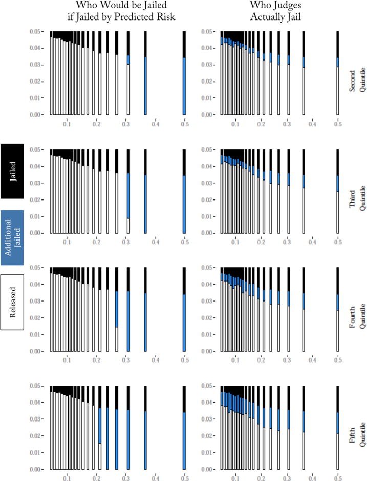
Notes: This figure shows where each of the quintiles of stricter judges in NYC select their marginal defendants (relative to the most lenient quintile), compared to how the algorithm would select marginal detainees. Within each panel, we divide the sample up into 20 bins by predicted crime risk (shown on the x-axis). The black segment at the top of each bar shows the share of each bin the most lenient quintile judges jail. In the top right-hand panel, we show which defendants the second-most-lenient quintile judges implicitly select to jail to get from the most lenient judge’s release rate down to their own lower release rate (blue), and who they continue to release (white). The left-hand top panel shows whom the algorithm would select instead. Each of the remaining rows shows the same comparison between the judge and algorithm decisions for the other less lenient judge quintiles.

The key finding from Figure VI is that as judges become stricter, they jail low risk individuals before high risk ones: marginal defendants are drawn from throughout the predicted risk distribution. The extent of misranking is sizable. All the additional jailing of the second quintile could be had by jailing everyone in the top 11.98 percentile of risk; yet only 33.2% of additional defendants come from this riskiest tail.³⁸ The third quintile of stringency could be achieved by jailing everyone in the top 14.10% of risk, and only 29.8% are drawn from there. For the fourth and fifth quintiles, the analogous numbers are the 18.56 and 28.45 percentiles; and 31.8% and 39.6%. A primary source of error is that all quintiles of judges misuse the signal available in defendant characteristics observable in our data: when prioritizing defendants for detention, many low risk defendants are ranked above high risk ones.

VI.C. Predicting Judicial Behavior

To better understand where and how judges are mistaken, it will be helpful to form a prediction of the judge’s choices, Ĵ. Let Ĵ_j(x) = E[ρ_j(x, z, w)|x] be the expected release probability for each individual based solely on the data available to judge j at the time of choice. Note that this predictive model of the judge never sees the outcome of whether the defendant committed crime, only who the judge released.

1. Which Cases are Hard?

We begin by examining where in the risk distribution judges are having the most trouble. While ex ante the answer is not obvious, looking at other domains can provide us with some initial intuition about what we might have expected. For example in education, studies find that principals do a good job identifying which teachers are in the tails of the performance distribution - the very high performers and the very low performers - but have a hard time distinguishing among teachers in the middle of the distribution (Jacob and Lefgren, 2008). Yet, our results for judge bail decisions run counter to this intuition.

We examine this question by investigating where in the predicted-risk distribution judges have the most uncertainty. What we observe is just a binary indicator of whether the judges released a given defendant i, which cannot convey much about judge uncertainy. However Ĵ(X_i), since it measures the probability of release, does quantify this uncertainty.

We find that judges struggle not so much with the middle of the distribution, but instead with one tail: the highest-risk cases. When we sort defendants into quintiles based on predicted crime risk, m(X_i), we see a much greater dispersion in predicted jailing probabilities Ĵ(X_i) among the highest-risk cases compared to the low-risk cases (Online Appendix Figure A.7). That is, judges treat many of these high-risk cases as if they are low risk. We have also examined the characteristics that define these tails. Judges are most likely to release high-risk people if their current charge is minor, such as a misdemeanor, and are more likely to detain low-risk people if their current charge is more serious (Online Appendix Table A.11). Put differently judges seem to be (among other things) overweighting the importance of the current charge.

2. Noisy Predictions

Putting aside for the moment the evaluation problem, let us first consider how Ĵ compares to the judge herself. To do this let us form a release rule

$${\rho }_{{\widehat{J}}_j}=1\text{if and only if}{\widehat{J}}_j\left(x\right)>k$$

where k is set to equalize its release rate to judge j’s. The difference in crime rates between the judge and $E\left[y{\rho }_{{\widehat{J}}_j}\right]-E\left[y{\rho }_j\right]$ which we can write as:

$$E\left[y\left({\rho }_{{\widehat{J}}_j}-{\rho }_j\right)\right]=E\left[x\left({\rho }_{{\widehat{J}}_j}-{\rho }_j\right)\right]+E\left[\overline{z}\left(x\right)-{\overline{z}}_j\left(x\right)\right]$$

We see it depends on two factors: (i) whether they release from some high-risk bins; and (ii) whether judges select well on unobservables, i.e. on whether the judge selects better or worse unobservables than the average in each x bin (which is what Ĵ achieves). It is clear that if h_j(x, z, w) = x + z then, conditionally on x, judges release the lower risk defendants; and hence ρ^j will outperform Ĵ. At the same time if human judgment is also influenced by w, unobservables not correlated with y, that can induce some high-risk bins to be released and possibly even selection on unobservables to be poor, allowing Ĵ to do better than j.

In practice, evaluating Ĵ suffers from the same issues as evaluating any m(x) rule and we will use contraction as above. We will do this in the same way we compared in Section IV.B. the judge to the algorithm. As before, we begin with the set of cases released by the most lenient quintile judges. We then jail additional defendants as we predict the judges would - jailing first those defendants with the highest predicted probability of judges jailing them. In other words, we begin by jailing those defendants who are released but whom we predicted have the highest probability of being jailed by the judges. (The difference with our previous comparison to the judges is that we had earlier jailed defendants by the algorithm’s predicted crime risk.)

We find that the predicted judge does better than the judges themselves. In Table VIII we quantify the crime reduction for the same increase in jailing, and we measure what jailing increase leads to the same crime reduction (the results are also plotted in Online Appendix Figure A.8). The predicted judge does significantly better. The second quintile of judges reduce crime by 9.9% by increasing the detention rate by 6.6 percentage points. The predicted judge would have achieved the same crime reduction by increasing the detention rate by only 4.7 percentage points (28.8% less than the judge); or alternatively, by increasing the detention rate by 6.6 percentage points we could have reduced crime by 13.4% (35.5% more than the judge). These are large gains by comparison: they represent more than half the gain achieved by using the algorithm trained on crime directly to release defendants. These results could in principle be due to a ‘wisdom of the crowd’ effect: Ĵ is not the predicted version of a single judge, but rather the prediction of many judges. Yet we find similar results using an algorithm trained on just a single judge’s caseload.³⁹

Table VIII.

Comparing Judges to the Predicted Judge using Contraction

	Judges		Predicted Judge (Ĵ)
	Relative to Most Lenient Quintile		To Achieve Judge’s
			Δ Crime	Δ Jail
	Δ Jail	Δ Crime	Δ Jail	Δ Crime
Second Quintile	0.066	−0.099	0.047	−0.134
Third Quintile	0.096	−0.137	0.068	−0.188
Fourth Quintile	0.135	−0.206	0.106	−0.254
Fifth Quintile	0.223	−0.307	0.166	−0.399

Notes: This table replicates the comparison of the algorithmic release rule to the decisions of less lenient quintile judges, but now using an algorithmic release rule based on a model that predicts the release decisions of the judges (our ‘predicted judge’ model). The first and second columns show the difference in jail rates and crime rates between the 2nd through 5th most lenient quintile judges compared to the most lenient quintile. The third column shows the increase in the jail population that would be required to meet the judges’ drop in crime if we jailed people in descending order of our prediction that the judges release a case. The fourth column shows the decline in crime that could be achieved if we increased the jail rate the same as the judges do, but detain people in ascending order of the judge predicted release probabilities.

Our results taken together suggests one reason why judge release decisions can be improved upon: Their actual decisions are noisy relative to a mean Ĵ that contains much more signal. In particular, this ‘noise’ appears to be due to unobservable variables, which unduly influence these decisions. Our data cannot tell us what these sources of ‘noise’ are but the behavioral science literature suggests that highly salient interpersonal information (such as the degree of eye contact that is made) can be overweighted, and that less salient but more informative data (like past behaviors) can be underweighted.

3. Decomposing the Sources of Judicial Error

A simple decomposition helps calibrate the extent of each source of judicial error. In particular, we focus on the crime gap between the judges’ and algorithm’s decisions: E[Y ρ^j] E[Y ρ^d]. For simplicity, empirically we calculate this difference in the context of our reranking policy simulation with α = 1. As in the previous section we can decompose this difference as (E[Y ρ^j]− E[Y ρ^Ĵ])+(E[Y ρ^Ĵ]− E[Y ρ^d]), the first term reflecting the inconsistency we have documented. Examples of this inconsistency include judges making exceptions to their usual decision rules based on irrelevant case characteristics or their mood at the time (w). We calculate this difference and display it in the Online Appendix, in Table A.12. This difference explains 25.9% of the gap in results between (ρ^j) and (ρ^d). It is worth noting that this is smaller than the gains we saw in Table VIII – it is possible that Ĵ is more useful for ranking marginal defendants than for a full reranking.

The predicted judge release rule ρ^Ĵ has two components. First, it groups people together as judges would: it treats (up to the need to tiebreak) all defendants within a Ĵ(x) cell identically. Second, it rank orders these cells as judges would: based on release rates E[R_j|Ĵ (x)]. But these are distinct errors. If judges had a simple linear model, but used the wrong sign on one of the binary variables, their groupings could be correct, but they would be misranking on one dimension. Our second decomposition differentiates between these two errors. We form a release rule that groups defendants as judges would, by Ĵ (x), but which then ranks them by E[Y|Ĵ (x)] (or more precisely E[m(x)|Ĵ(x)]). We see that this release rule is able to achieve 36.4% of the total performance gain of (ρ^d) versus (ρ^j), or put differently adds another 10.5% of the overall ρ^d gain relative to what is achieved by our standard predicted judge rule, Ĵ(x).

The remaining judge error is due to judges having the wrong underlying structure for which defendants are similar to one another with respect to risk. This could arise if for example there are key case characteristics that judges completely ignore, or interactions between variables that judges do not consider.⁴⁰ Our decomposition is only approximate, since our model for the judge’s decisions Ĵ(x) is not perfect.⁴¹ But it is telling that fully 63.6% of the gap in performance between (ρ^j) and (ρ^d) is left unexplained by the other components of our decomposition.

VII. CONCLUSION

The bail example highlights the value of solving social science problems of the type:

$$\text{Data}\to \text{Prediction}\to \text{Decision}$$

Machine-learning applications typically focus solely on the Data → Prediction link. The objective is to search through different candidate prediction functions and identify the one with the greatest prediction accuracy - a ‘bake off.’ Algorithm performance tends to be quantified on predictive value. The bail example, though, illustrates why understanding the Prediction → Decision link is at least as important. Looking past prediction quality to decision quality is what makes clear the problems of selective labels and omitted-payoff biases. Good predictors do not necessarily improve decisions. There is significant distance between constructing a prediction algorithm and knowing that a decision aid based on it can improve outcomes.

It is instructive to compare the state of the art for introducing data-driven decision aids with how new drug therapies are brought to market. Before any new drug can be sold the Food and Drug Administration (FDA) requires several stages of testing. Phase 0 and Phase 1 trials demonstrate basic safety of the drug, while Phase 2 trials compare at medium scale and for easily measured outcomes the effects of the new drug to either placebo or current best practice. If a drug passes, it is subject to a larger scale Phase 3 trial that quantifies key clinical outcomes. Current machine-learning practice of establishing predictive validity is analogous to passing a Phase 0 or 1 trial. As with drugs, going directly from a Phase 0 or 1 trial to market risks doing social harm.

We view our results, with their focus on payoffs and counterfactual evaluation of the decision aids, as the equivalent of a Phase 2 trial. They show promising impacts. At the same time, they leave several open questions that would require the analogue of a Phase 3 trial. Such a trial would begin with an explicit discussion of the key objectives for any new decision aid, reducing risk of omitted-payoff bias. The trial itself would quantify how judges interact with the decision aid. Sometimes judges largely ignore these tools, as in New York City, perhaps because the six-item checklist risk tool they use has limited predictive accuracy (NYC CJA 2016). But in other cases where algorithms may be more accurate they do appear to be used, as in the Philadelphia bail experiment (Goldkamp and Gottfredson, 1984, 1985) and more recently when parole boards get machine-learning-based tools (Berk, 2017). The design of decision aids requires some way to ensure judges override when they have signal rather than when they are simply adding noise (the ‘override problem’). Finally, a large-scale trial is the only way to quantify general equilibrium effects. For example in our application both defendant and judges’ behavior could change if all cases were filtered through a predictive model (for example if judges change their willingness to dispose of cases at the bail hearing).

Prediction policy problems are not only socially important, they are also scientifically interesting. Predictive algorithms can serve as a behavioral diagnostic, helping to understand the nature of human error. Though the data we have were somewhat limited in this regard, algorithms applied to richer data might produce novel behavioral insights. Progress on these problems will require a synthesis of multiple perspectives, both the techniques of machine learning as well as behavioral science and economics. Experimental tools have been invaluable for understanding and improving human decisions. If our findings are any indication, predictive tools could prove similarly effective.

References

- Abaluck Jason, Agha Leila, Kabrhel Chris, Raja Ali, Venkatesh Arjun. The determinants of productivity in medical testing: Intensity and allocation of care. American Economic Review. 2016;106:3730–3764. [PubMed] [Google Scholar]
- Abrams David S, Rohlfs Chris. Optimal bail and the value of freedom: Evidence from the Philadelphia bail experiment. Economic Inquiry. 2011;49:750–770. [Google Scholar]
- Aizer Anna, Doyle Joseph., Jr Juvenile incarceration, human capital and future crime: Evidence from randomly-assigned judges. Quarterly Journal of Economics. 2015;130:759–803. [Google Scholar]
- Athey Susan, Katz Lawrence F, Krueger Alan B, Levitt Steven, Poterba James. What does performance in graduate school predict? Graduate economics education and student outcomes. American Economic Review, Papers and Proceedings. 2007;97:512–518. [Google Scholar]
- Athey Susan, Imbens Guido. Recursive partitioning for heterogeneous causal effects. Proceedings of the National Academy of Sciences. 2016;113:7353–7360. doi: 10.1073/pnas.1510489113. [DOI] [PMC free article] [PubMed] [Google Scholar]
- Banko Michele, Brill Eric. Proceedings of the 39th Annual Meeting on Association for Computational Linguistics. Association for Computational Linguistics; 2001. Scaling to very very large corpora for natural language disambiguation. [Google Scholar]
- Belloni Alexandre, Chernozhukov Victor, Hansen Christian. High-dimensional methods and inference on structural and treatment effects. The Journal of Economic Perspectives. 2014;28:29–50. [Google Scholar]
- Berk Richard. Criminal Justice Forecasts of Risk: A Machine Learning Approach. New York, NY: Springer; 2012. [Google Scholar]
- Berk Richard. An impact assessment of machine learning risk forecasts on parole board decisions and recidivism. Journal of Experimental Criminology. 2017;13:193–216. [Google Scholar]
- Berk Richard, Bleich Justin. Forecasts of violence to inform sentencing decisions. Journal of Quantitative Criminology. 2015;30:9–96. [Google Scholar]
- Berk Richard, Bleich Justin, Kapelner Adam, Henderson Jaime, Barnes Geoffrey, Kurtz Ellen. Using regression kernels to forecast a failure to appear in court. Working Paper. 2014 [Google Scholar]
- Bhuller Manudeep, Dahl Gordon B, Løken Katrine V, Mogstad Magne. Incarceration, recidivism and employment. Working Paper. 2016 [Google Scholar]
- Black Fischer. Noise. The Journal of Finance. 1986;41:528–543. [Google Scholar]
- Bordalo Pedro, Gennaioli Nicola, Shleifer Andrei. Salience theory of choice under risk. The Quarterly Journal of Economics. 2012;127:1243–1285. [Google Scholar]
- Bushway Shawn, Smith Jeffrey. Sentencing using statistical treatment rules: What we don’t know can hurt us. Journal of Quantitative Criminology. 2007;23:377–387. [Google Scholar]
- Chalfin Aaron, Danieli Oren, Hillis Andrew, Jelveh Zubin, Luca Michael, Ludwig Jens, Mullainathan Sendhil. Productivity and selection of human capital with machine learning. American Economic Review: Papers and Proceedings. 2016;106:124–127. [Google Scholar]
- Dawes Robyn M, Faust David, Meehl Paul E. Clinical versus actuarial judgment. Science. 1989;243:1668–1674. doi: 10.1126/science.2648573. [DOI] [PubMed] [Google Scholar]
- Dawes Robyn M. A case study of graduate admissions: Application of three principles of human decision making. American Psychologist. 1971;26:180–188. [Google Scholar]
- Dawes Robyn M. The robust beauty of improper linear models in decision making. American Psychologist. 1979;34:571–582. [Google Scholar]
- Di Tella Rafael, Schargrodsky Ernesto. Criminal recidivism after prison and electronic monitoring. Journal of Political Economy. 2013;121:28–73. [Google Scholar]
- Dietvorst Berkeley J, Simmons Joseph P, Massey Cade. Algorithm aversion: People erroneously avoid algorithms after seeing them err. Journal of Experimental Psychology: General. 2015;144:114–126. doi: 10.1037/xge0000033. [DOI] [PubMed] [Google Scholar]
- Dobbie Will, Goldin Jacob, Yang Crystal. The effects of pre-trial detention on conviction, future crime, and employment: Evidence from randomly assigned judges. NBER Working Paper. 2016;22511 [Google Scholar]
- Donohue John J. Assessing the relative benefits of incarceration: Overall changes and the benefits on the margin. In: Raphael Steve, Stoll Michael A., editors. Do Prisons Make Us Safer? Benefits and Costs of the Prison Boom. New York, NY: Russell Sage; 2009. [Google Scholar]
- Friedman Jerome H. Greedy function approximation: A gradient boosting machine. Annals of Statistics. 2001;29:1189–1232. [Google Scholar]
- Goldkamp John S, Gottfredson Michael R. (National Institute of Justice Research Report NCJ95109).Judicial Decision Guidelines for Bail: The Philadelphia Experiment. 1984 [Google Scholar]
- Goldkamp John S, Gottfredson Michael R. Judicial Decision Guidelines for Bail: The Philadelphia Experiment, 1981-1982. 1985a;ICPSR08358-v1 [Google Scholar]
- Goldkamp John S, Gottfredson Michael R. Policy Guidelines for Bail: An Experiment in Court Reform. Philadelphia, PA: Temple University Press; 1985b. [Google Scholar]
- Grove William M, Zald David H, Lebow Boyd, Snitz Beth E, Nelson Chad. Clinical versus mechanical prediction: A meta-analysis. Psychological Assessment. 2000;12:19–30. [PubMed] [Google Scholar]
- Gupta Arpit, Hansman Christopher, Frenchman Ethan. The heavy costs of high bail: Evidence from judge randomization. Columbia University Working Paper. 2016 [Google Scholar]
- Harcourt Bernard E. Risk as a proxy for race: The dangers of risk assessment. Federal Sentencing Reporter. 2015;27:237–243. [Google Scholar]
- Hastie Trevor, Tibshirani Robert, Friedman Jerome. The Elements of Statistical Learning. Berlin: Springer; 2009. [Google Scholar]
- Henrichson Christian, Rinaldi Joshua, Delaney Ruth. The Price of Jails: Measuring the Taxpayer Cost of Local Incarceration. New York, NY: Vera Institute of Justice; 2015. [Google Scholar]
- Holder Eric. Prepared remarks. 2014 http://www.justice.gov/opa/speech/attorney-general-eric-holder-speaks-national-association-criminal-defense-lawyers-57th.
- Jacob Brian A, Lefgren Lars. Principals as agents: Subjective performance assessment in education. Journal of Labor Economics. 2008;26:101–136. [Google Scholar]
- Jung Jongbin, Concannon Connor, Shroff Ravi, Goel Sharad, Goldstein Daniel G. Simple rules for complex decisions. Stanford University Working Paper. 2017 [Google Scholar]
- Kahneman Daniel, Rosenfield Andrew M, Gandhi Linnea, Blaser Tom. NOISE: How to overcome the high, hidden cost of inconsistent decision making. Harvard Business Review. 2016;94:38–46. [Google Scholar]
- Kahneman Daniel, Tversky Amos. Judgment under uncertainty: Heuristics and biases. Science. 1974;185:1124–1131. doi: 10.1126/science.185.4157.1124. [DOI] [PubMed] [Google Scholar]
- Kleinberg Jon, Lakkaraju Himabindu, Leskovec Jure, Ludwig Jens, Mullainathan Sendhil. Replication Data for: ‘Human Decisions and Machine Predictions’. Harvard Dataverse. 2017 doi: 10.7910/DVN/VWDGHT. [DOI] [PMC free article] [PubMed] [Google Scholar]
- Kleinberg Jon, Ludwig Jens, Mullainathan Sendhil, Obermeyer Ziad. Prediction policy problems. American Economic Review, Papers and Proceedings. 2015;105:491–495. doi: 10.1257/aer.p20151023. [DOI] [PMC free article] [PubMed] [Google Scholar]
- Kling Jeffrey R. Incarceration length, employment, and earnings. American Economic Review. 2006;96:863–876. [Google Scholar]
- Lakkaraju Himabindu, Leskovec Jure, Kleinberg Jon, Mullainathan Sendhil. A bayesian framework for modeling human evaluations. Proceedings of the 2015 SIAM International Conference on Data Mining. 2015 [Google Scholar]
- Lakkaraju Himabindu, Rudin Cynthia. Learning cost-effective and interpretable treatment regimes. Proceedings of Machine Learning Research. 2017;54:166–175. [Google Scholar]
- Lakkaraju Himabindu, Kleinberg Jon, Leskovec Jure, Ludwig Jens, Mullainathan Sendhil. The Selective labels problem: Evaluating algorithmic predictions in the presence of unobservables. KDD Conference Proceedings. 2017 doi: 10.1145/3097983.3098066. [DOI] [PMC free article] [PubMed] [Google Scholar]
- Laqueur Hannah, Copus Ryan. Synthetic crowdsourcing: A machine-learning approach to the problems of inconsistency and bias in adjudication. Working Paper. 2016 [Google Scholar]
- Leslie Emily, Pope Nolan. The unintended impact of pretrial detention on case outcomes: Evidence from NYC arraignments. Working Paper. 2016 [Google Scholar]
- Logg Jennifer. Theory of Machine: When Do People Rely on Algorithms? Harvard Business School Working Paper. 2017 [Google Scholar]
- Meehl Paul E. Clinical versus Statistical Prediction: A Theoretical Analysis and a Review of the Evidence. Minneapolis, MN: University of Minnesota Press; 1954. [Google Scholar]
- Mendel Brock, Shleifer Andrei. Chasing noise. Journal of Financial Economics. 2012;104:303–320. [Google Scholar]
- Mueller-Smith Michael. The criminal and labor market impacts of incarceration. University of Michigan Working Paper. 2015 [Google Scholar]
- Mullainathan Sendhil, Spiess Jann. Machine learning: an applied econometric approach. Journal of Economic Perspectives. 2017;31:87–106. [Google Scholar]
- Murphy Kevin P. Machine Learning: A Probabilistic Perspective. Cambridge, MA: MIT Press; 2012. [Google Scholar]
- New York City Department of Corrections. NYC DOC at a Glance. New York, NY: New York City Department of Corrections; 2012. http://www.nyc.gov/html/doc/downloads/pdf/doc_at_a_glance.pdf. [Google Scholar]
- New York City Criminal Justice Agency, Inc. Annual Report 2014. New York, NY: New York City Criminal Justice Agency Inc; 2016. [Google Scholar]
- Ohlin Lloyd E, Duncan Otis Dudley. The efficiency of prediction in criminology. American Journal of Sociology. 1949;54:441–452. doi: 10.1086/220398. [DOI] [PubMed] [Google Scholar]
- Phillips Mary T. A Decade of Bail Research in New York City. New York, NY: New York City Criminal Justice Agency; 2012. [Google Scholar]
- Rosenbaum Paul R, Rubin Donald B. Assessing sensitivity to an unobserved binary covariate in an observational study with binary outcome. Journal of the Royal Statistical Society, Series B (Methodological) 1983;45:212–218. [Google Scholar]
- Shiller Robert J. Do stock prices move too much to be justified by subsequent changes in dividends? American Economic Review. 1981;71:421–436. [Google Scholar]
- Starr Sonja B. Evidence-based sentencing and the scientific rationalization of discrimination. Stanford Law Review. 2014;66:803–872. [Google Scholar]
- Stevenson Megan. Distortion of justice: How the inability to pay bail affects case outcomes. University of Pennsylvania Working Paper. 2016 [Google Scholar]
- Tan Chenhao, Lee Lillian, Pang Bo. The effect of wording on message propagation: Topic- and author-controlled natural experiments on Twitter. Proceedings of the 52nd Annual Meeting of the Association for Computational Linguistics (ACL 2014) 2014 [Google Scholar]
- Toborg Mary A. Pretrial release: A national evaluation of practices. Washington, DC: National Institute of Justice; 1981. [Google Scholar]
- Toborg Mary A. Pretrial release practices in the United States, 1976-1978. Ann Arbor, MI: Inter-university Consortium on Political and Social Research; 1997. 2nd ICPSR edition. ICPSR07972.v2. [Google Scholar]
- US Department of Justice, Bureau of Justice Statistics. State Court Processing Statistics, 1990–2009: Felony Defendants in Large Urban Counties [computer file], Conducted by Pretrial Justice Institute (formerly, the Pretrial Services Resource Center) Ann Arbor, MI: Inter-university Consortium for Political and Social Research; 2014. ICPSR02038-v5. [Google Scholar]
- Varian Hal R. Big data: New tricks for econometrics. Journal of Economic Perspectives. 2014;28:3–28. [Google Scholar]
- Yeomans Mike, Shah Anuj, Kleinberg Jon, Mullainathan Sendhil. Making Sense of Recommendations. Harvard University Working Paper. 2016 [Google Scholar]
- Zeng Jiaming, Ustun Berk, Rudin Cynthia. Interpretable classification models for recidivism prediction. Journal of the Royal Statistical Society, Series A (Society) 2017;180:689–722. [Google Scholar]
Associated Data
This section collects any data citations, data availability statements, or supplementary materials included in this article.