A quasi-3D compartmental multi-scale approach to detect and quantify diseased regional lung constriction using spirometry data

Abstract

Spirometry is a widely used pulmonary function test to detect the airflow limitations associated with various obstructive lung diseases, such as asthma, chronic obstructive pulmonary disease (COPD), and even obesity-related complications. These conditions arise due to the change in the airway resistance, alveolar compliance, and inductance values. Currently, zero-dimensional (0D) compartmental models are commonly used for calibrating these resistance, compliance, and inductance values, i.e., solving the inverse spirometry problem. However, 0D compartments cannot capture the flow physics or the spatial geometry effects, thereby generating a low fidelity prediction of the diseased lung. Computational fluid dynamics (CFD) models offer higher fidelity solutions but may be impractical for certain applications due to the duration of these simulations. Recently, a novel, fast-running and robust Quasi-3D (Q3D) wire model for simulating the airflow in the human lung airway was developed by CFD Research Corporation (CFDRC). This Q3D method preserved the 3D spatial nature of the airways and was favorably validated against CFD solutions. In the present study, the Q3D compartmental multi-scale combination is further improved to predict regional lung constriction of diseased lungs using spirometry data. The Q3D mesh is resolved up to the eighth lung airway generation. The remainder of the airways and the alveoli sections are modeled using a compartmental approach. The Q3D geometry is then split into different spatial sections and the resistance values in these regions are obtained using parameter inversion. Finally, the airway diameter values are then reduced to create the actual diseased lung model, corresponding to these resistance values. This diseased lung model can be used for patient-specific drug deposition predictions and the subsequent optimization of the orally inhaled drug products.

1. Introduction

Obstructive lung diseases such as asthma and chronic obstructive pulmonary disease (COPD) are estimated to affect around 350 million people worldwide [20, 30]. These diseases are also linked to around 3 million deaths each year globally [30]. Some of the major causes for airflow limitation are airway smooth muscle hypertrophy and airway remodeling [2,5], blockage of the airways with mucus and inflammatory debris [6], airway closure due to surfactant dysfunction [29], and loss of alveolar attachments causing reduced lung elastic recoil [21].

While the airflow limitation is the result of the above-mentioned mechanisms, the mathematical models designed to understand these mechanisms operate using first principle conservation equations that mainly use three factors to differentiate a healthy lung from its diseased counterpart: (i) the airway and alveolar resistance values, (ii) the alveolar compliance values, and the (iii) alveolar inductance values. These mechanical/structural properties are sufficient to assess the general health of the lung.

In the past, several research studies have been carried out to assess lung health using the measured flowrate and pressure obtained from spirometers [25,11,8,1]. These studies determine the lung system parameters from the raw spirometry data, using parameter inversion techniques. Parameter optimization is the selection of best parameters (in this case the lung system parameters) so as to minimize the deviation from the measured data (in this case the available spirometry data). Generally, such studies lump the lung airway regimes (for instance as upper, central, peripheral, and alveolar) into zero-dimensional (0D) compartmental blocks and then invert for the mechanical/structural properties (resistance, compliance, and inductance values). The limitations of this approach include (i) the assumption that the diameters and lengths are constant in a particular airway section, (ii) a 1:2 branching (i.e., bifurcation) in accordance with the Typical Path Lung (TPL) model [28], thus neglecting the actual structure of the lung, (iii) inaccurate representation of the airway geometry (i.e., the three-dimensional geometrical structure) and its effect on deposition, and (iv) uniform division of the flow rate when the parent airway branches into two daughter airways, thus failing to rigorously address local inflammations for instance in a particular lung lobe. Hence, the culmination point from these 0D compartmental model-based inversions is reached with the lumped resistance values over several airway sections, along with the lumped compliance and inductance values (i.e. a single resistance, compliance and inductance value over several airway sections). While these are certainly useful in predicting the overall lung health, they neither provide the injury location on a spatial basis nor can be accessed by the research community toward optimized treatment of that particular patient.

For similar endpoints, multiple other studies have used 3D computational fluid dynamics (CFD) models. This approach involves obtaining the STL (STereoLithography) surface mesh from computed tomography (CT) scans or other images, creating volumetric meshes inside the lung domain and then solving the conservation equations in each computational cell. In CFD, a large number of degrees of freedom (DOF), or computational cells is required in order to accurately depict the lung geometry and to minimize the spatial discretization error. Similarly, a small enough time step is also required in order to minimize the temporal discretization error (i.e. the error resulting from the fact that a function of a continuous variable is represented in the computer by a finite number of evaluations in time). The above constraints necessitate the lung mesh to have more than a million DOF and for the time step to be small enough to cause the total computational time to be on the order of days (even with parallel computing) for simulating a few breathing cycles, i.e., running the forward problem. A typical inversion procedure will involve invoking the forward problem (with continuous changes to the parameters) several times, so as to obtain the descent to the correct parameters (details of the inversion procedure used in CoBi can be obtained from previous publications [12,13]). Hence, running an inverse spirometry simulation will require several months for completion, thereby making this approach impractical. Nonetheless, the CFD approach can efficiently capture the detailed flow phenomena like (i) localized vortices and recirculation regimes [27,15], (ii) regions of high turbulence [27,10], and (iii) the flow path lines, thereby being an invaluable driver for specialized applications like the particle transport simulations [14] or drug delivery simulations [15, 27]. However, the above-mentioned details are not necessary to predict the pressures or flow rates in the airway.

A third approach, namely the Quasi-3D (Q3D) approach, was presented by Kannan et al [16] for modeling the airflow in human lungs. The Q3D approach is a robust, time efficient, and adaptable procedure where a high-fidelity surface CFD type mesh is contracted to a structure of connected 1D wires, with well-defined radii. The surface mesh for the human lung airway was obtained from the Zygote Body web application [32]. These are based on medical scans of a 50th percentile individual [32]. The nasal region was truncated. This surface mesh has around six to eight airway generations, which is shown in Figure 1a. The surface mesh and the wire mesh are shown in Figure 1. It can be seen that the lung geometry details are still preserved. The wire mesh has 1116 cells (DOF). The mouth region is not a high-fidelity representation of the original surface mesh since that region is sufficiently complicated and hence cannot be accurately represented by a cylindrical geometry.

Figure 1.

Lung airway model. Case (a) high fidelity lung airway surface mesh obtained from the zygote body list; it is used to extract the center line and radius of the lung airways. Case (b): Q3D wire mesh for the same region constructed on the extracted information from the lung airways.

A 3D CFD model built using the surface mesh would result in approximately 2–5 million cells and solving the transport equations on such a mesh would require several parallel machines and would result in several days of simulation time. In comparison, the Q3D wire mesh can produce a result which is quantitatively’ acceptable (i.e. a maximum error of around 10–15%) within a few minutes of (forward run) simulation time as shown in our published study [16].

The conservation equations are then solved in each of these wires. The resulting simulations are extremely fast (compared to using CFD simulations) due to the quasi-3D nature of the wire mesh, with the Q3D approach being 3,000–25,000 times faster than the CFD simulations. The Q3D simulations also converge more easily, since there are no badly skewed cells (i.e. the internal angles of the computational cell being much larger/smaller than the ideal equi-angular polyhedron) or highly stretched cells (i.e. the ratio of the largest to the smallest edges in that computational cell being very high), thereby requiring fewer steady/unsteady sweeps during a steady/transient simulation. Figure 2 shows the pressures obtained using the two methods when a steady flow rate of 5.0 L/min was prescribed. The pressure at the mouth was set to atmospheric and the outlet velocity was set at the outlets. This flow rate is within the laminar range. It can be seen in Figure 2 that the predicted pressures in the different regions of the airway using full 3D CFD and Q3D are similar; the Q3D simulation was 18000 times faster than the 3D CFD model.

Figure 2.

Pressure distribution (in Pascal) in the healthy lung airway model, during a laminar simulation (Q = 5L/min). Case (a) Solution from a full CFD simulation; Case (b): Solution from a Q3D simulation, with its legend range; Case (c): Solution from a Q3D simulation, with the legend rage of the CFD simulation.

In the present study, we used a Q3D compartmental multi-scale approach to reconstruct the regional lung properties of diseased lungs from the raw spirometry data, using parameter inversion techniques. More specifically, the proposed method is limited to the diseased cases where changes in FEV1 (Forced expiratory volume, in one second) is expected to relate to morphological changes in the airway. A schematic of this multiscale computational domain is shown in Figure 3. The spatially resolved section ends at around the eighth lung generation (G8). Please note that the accepted norm is to number the trachea as the zeroth generation. The remainder of the airways (G9–G15) and the alveoli (G16–G24) are lumped into two individual compartments. The compartmental mechanical/structural properties (resistance, compliance, and inductance values: detailed definitions can be obtained from Bates et al. [1]) and the resistance values in the various sections of the Q3D geometry (to a desired level of discretization) are obtained by the optimization procedure. The resistance in the Q3D geometry is then translated to a corresponding diameter reduction, thereby creating the actual diseased lung model. This actual diseased lung model can be used for exploring/optimizing personalized drug delivery treatment options for that patient. These details will be provided in later sections.

Figure 3.

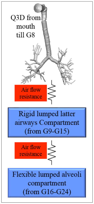
Multi-scale Q3D-compartment computational domain. The Q3D starts at the mouth and ends at around the eighth lung generation.

This paper is organized as follows. In section 2, we give a detailed introduction to this multiscale Q3D-compartment setup, including the equations and the variables to be calibrated, with the aid of an actual spirometry dataset. Obtaining the final diseased lung model using the computed Q3D resistance is discussed in section 3. A second calibration is performed in section 4, using a different spirometry dataset. Finally, conclusions from this study are summarized in section 5.

2. Multiscale Q3D-compartment model setup

The Q3D model

In many biomedical and engineering problems, the physical process occurs in networks of pipes, cables, wires, or other 1D structures. The best examples are the human vascular system, lymphatic network, neurons with a network of dendrites and axons, microfluidic channels in biochips and air flow transport in lungs. As mentioned before, full-fledged 3D computational simulations of such large tubing structures are difficult to perform and may not always provide an advantage over a 1D model of a tubing network distributed in a 3D space in the prediction of certain physiological parameters. Kannan et al [16] have developed a Quasi-3D (Q3D) wire model to solve such problems. The important advantages of this Q3D model over full 3D simulations are the ease of model setup, less computation time, and easy to link with compact models such as spring/mass/damper devices, valves, pumps, controllers, or certain compartmental models. Additional details, including the wire-generation process and the accuracy/speedup comparisons for a host of simulation test cases, can be obtained from Kannan et al [16].

For the sake of completeness, we will present compare the Q3D and CFD outlet pressures, for a highly transient simulation. The inhalation profile described by Nishi et al [23] was used in this research endeavor. As shown in Figure 4, a breathing cycle comprises of an inhalation period of 1.5 seconds and an exhalation period of 2.1 seconds. We will compare the Q3D and CFD outlet pressures (average of nearly 120+ outlets). The pressure was set to atmospheric in the mouth inlet. A dynamic volumetric flux boundary condition (i.e. depending on the current flow rate) was prescribed at the lung outlets. A timestep of 0.02 seconds was employed. Figure 5 shows the Q3D and CFD averaged pressure plots as a function of time. Some remarks: (a) In general, the CFD and Q3D pressures are remarkably close, (b) The CFD pressure plots, show some oscillations at the peak flow rates, probably due to some vortex shedding/recirculation. This is not present in the Q3D simulations and (c) The Q3D and CFD pressures match both in the inhale, exhale and the intermediate stage between them. Nevertheless, the pressure magnitudes are very similar, thus showing that the Q3D method can be used for Spirometry type computations, wherein the pressure values are the main indicators of the lung health (not the secondary physics like vorticity or recirculation). Figure 6 shows the Q3D and CFD surface pressure plots at two different time stages. Once again, they are numerically very similar.

Figure 4.

A realistic volumetric flow rate for humans. Figure adapted from Nishi et al [23]

Figure 5.

Averaged outlet pressure, for the realistic transient flow conditions, prescribed by Nishi et al [23]

Figure 6.

Pressure distribution (in Pascal) in the healthy lung airway model, for a transient realistic breathing profile. Case (a) CFD solution at 0.4s; Case (b): Q3D solution at 0.4s; Case (c): CFD solution at 1.6s and Case (d): Q3D solution at 1.6s.

The authors would like to admit that complicated secondary flows, the local vorticity creation at the ridges and other detailed features cannot be captured by the Q3D model. However, it can accurately predict the local fluid pressures and provide accurate transport effects. Hence, it can be applied in areas wherein the effect of the secondary flows are not important like spirometry and the drug transport in the surface lining liquid [17].

The compartmental model

The Q3D model was created from the Zygote5 STL surface mesh. This geometry has around 6–8 airway generations. This STL surface mesh was originally obtained from a CT scan. Due to insufficient resolution of the CT scans, the airway geometry was only extended up to G8 in Q3D. The rest of the airways (G9–G15) and the alveoli (G16–G24) were simulated using two lumped compartments: the latter airway compartment (G9–G15) and the alveoli compartment (G16–G24). The latter airway compartment is rigid and the alveolar compartment is flexible. NOTE: The airways are practically rigid. Chovancova et al. [3] have shown that the pressure difference even in the case of forced inhalation and exhalation is at the most 80 Pa. Prakash et al. [26] have shown from in vitro studies that the diameter change for the airways is less than 1.2% even for a pressure difference of 500 Pa. While it is possible that some of the terminal latter airways might have some compliance they are neglected in the context of these engineering simulations.

The alveolar and the latter airway compartmental equations are as follows:

$$\begin{gathered} \frac{\partial V_{AL}}{\partial t}=Q \\ {P}_{AL}=P_{PL}+\frac{(V_{AL}-V_{AL0})}{{\mathit{CAP}}_{AL}} \\ {P}_{\mathit{LAW}}=\begin{array}{l}Q\ge 0:(Q\ast R{L}_P)+P_{AL}+(I\ast \frac{\partial Q}{\partial t}),\hfill \\ Q<0:(Q\ast R{L}_N)+P_{AL}+(I\ast \frac{\partial Q}{\partial t})\hfill \end{array} \\ {P}_{ZE}=\begin{array}{l}Q\ge 0:(Q\ast R{P}_P)+P_{\mathit{LAW}}\hfill \\ Q<0:(Q\ast R{P}_N)+P_{\mathit{LAW}}\hfill \end{array} \end{gathered}$$ (1)

where, V_AL is the alveolar volume at any given time, V_AL0 is the basal alveolar volume (when the flow rate is zero), Q is the flow rate, P_AL is the alveolar pressure, P_PL is the pressure of the layer covering the alveoli, CAP_AL is the alveolar capacitance, P_LAW is the pressure at the end of the latter airways compartment, RL_P is the positive linear resistance of the section connecting the latter airways and the alveoli, RL_N is the negative linear resistance of the section connecting the latter airways and the alveoli, I is the inductance of the section connecting the latter airways and the alveoli, RP_P is the positive linear resistance of the section connecting the latter airways and the Q3D model, RP_N is the negative linear resistance of the section connecting the latter airways and the Q3D model, and P_ZE is the pressure to be applied to at the outlets of the Q3D model.

In this model, we have included the dynamic effects of the flow on the pressure. It is evident that a static formulation will remove the effect of impedance on the pressure. In fact, some of the reported compliance values in literature are from static conditions and hence are unreliable [9]. We have also assumed a value of zero Pascal (gauge pressure) for P_PL.

Spirometry computation

In this effort, the Q3D domain is split into five sub-sections: the OPL (Oral-Pharyngeal-Laryngeal) region, the tracheal region, the first generation to the right, the first generation to the left, and the lower airway section. Figure 7 shows the color-coded pictorial shading of these regions on the Q3D geometry. Each of these regions is provided with an additional numerical resistance, in addition to the resistance due to the viscous and turbulent stresses, to account for the lumen shrinkage in that region. This numerical resistance is applied to each computational cell in that sub-section. The above resistances (excluding that of the OPL region, since there is lumen reduction in that sub-section), along with RL_P, RL_N I, CAP_AL, RP_P and RP_N need to be calibrated for the diseased case.

Figure 7.

Color coded pictorial shading of the different sub-sections of the Q3D domain.

The first optimization case study used the data set provided by Pankow et al [24]. The test subject was from an obese test set, which had a Body Mass Index (BMI) of 44±5 kg/m². Some of the members in the test set had mild obstructive sleep apnea. Figure 8 shows the pressure and flow rate readings of this test subject [24]. The domain specific resistance (corresponding to the lumen shrinkage) for this test subject is obtained through parameter optimization. The flowrate presented in Figure 8 is used as the inlet boundary condition for the simulation. The lung geometrical and physical properties need to be calibrated to obtain the mouth pressure shown in Figure 8.

Figure 8.

Flow rate and pressure at the mouth airway opening (ao) for a test subject. Data digitized from Pankow et al [24]. Case a: pressure readings; Case b: flow rate measurements.

The flow solver in our numerical suite CoBi (Computational Biology) uses a pressure-based (SIMPLE algorithm) finite volume method that is second order accurate in space and has first and second order temporal integration schemes. The GMRES and the Algebraic MultiGrid (AMG) algorithms were employed for solving the linearized [A][x]=[b] problem for the velocity and pressure corrections equations in the SIMPLE algorithm respectively. For inhalation volumetric flow rates exceeding 12 L/min, the flow field can be turbulent in several locations, including the laryngeal region and for a few lung airway generations [10,19,14]. For flow rates exceeding 20 L/min most regions in the geometry have the local Reynolds number much higher than the critical value needed to trigger turbulence, for instance, the authors have observed a Reynolds number of 5,500 in the trachea region when the flow rates are greater than 20 L/min. The turbulent stresses were modeled by the use of a turbulent viscosity, computed using the Smagorinsky closure formulation. More details on the CoBi numerical suite, including the individual modules, formulations, and applications can be obtained from previous publications [12,13,14,18]. This flow solver will be invoked concurrently with the ODE solver (for the compartmental equations).

The Levenberg–Marquardt optimization routine in CoBi was invoked to optimize the parameters, for this test subject. Details on this gradient-based local optimizer, including its efficiency, accuracy, and robustness can be obtained from earlier publications [12,13]. The optimized values for this example simulation are provided in Table 1. Figure 9 shows the pressure at the mouth using this multiscale Q3D-compartment approach and the experimental measurements. They are in good accord with each other.

Table 1.

Optimized parameter set for the experimental data set provided by Pankow et al [24]

Parameters	Values
RLP (positive linear resistance of the section connecting the latter airways and the alveoli)	$78.44\frac{Pa\ast s}{\mathit{liter}}$
RLN (negative linear resistance of the section connecting the latter airways and the alveoli)	$121.617\frac{Pa\ast s}{\mathit{liter}}$
I (inductance of the section connecting the latter airways and the alveoli)	$3.697\frac{Pa\ast s\ast s}{\mathit{liter}}$
CAPAL (alveolar capacitance)	$0.9\frac{\mathit{liter}}{\mathit{cmH}2O}$
RPP (positive linear resistance of the section connecting the latter airways and the Q3D model)	$58.20\frac{Pa\ast s}{\mathit{liter}}$
RPN (negative linear resistance of the section connecting the latter airways and the Q3D model)	$100.12\frac{Pa\ast s}{\mathit{liter}}$
Q3D-resistancetrachea	$2.2185\mathrm{e}+001\frac{Pa\ast s}{m^2}$
Q3D-resistancegen1L	$2.6166\mathrm{e}+001\frac{Pa\ast s}{m^2}$
Q3D-resistancegen1R	$3.1851\mathrm{e}+001\frac{Pa\ast s}{m^2}$
Q3D-resistanceLowerAirways	$1.6254\mathrm{e}+001\frac{Pa\ast s}{m^2}$

Figure 9.

Pressures at the mouth using the multiscale Q3D-compartment approach and the experimental measurements. Experimental data from Pankow et al [24].

3. Obtaining the diseased geometry from the numerical resistances

The existing spirometry optimization procedures can neither provide the injury location (i.e., spatially) nor the diseased lung geometry [1, 25]. The ultimate aim of this research is to obtain the geometrical shape and structure of the diseased lung, so as to use it for optimizing the treatment of that particular patient by conducting high-fidelity drug particle transport simulations.

The full flow resistance in wire/pipe is defined as

$$R_{\mathit{FULL}}=\frac{\mathrm{\Delta }P}{Q},$$ (2)

where, ΔP is the pressure difference in that wire section and Q is the flowrate in that section. This resistance can be computed using the Hagen-Poiseuille equation:

$$R_{\mathit{FULL}}=\frac{8\mu L}{\pi {\mathit{Rad}}^4},$$ (3)

where, μ is the dynamic viscosity of the fluid, L is the length of the wire segment, and Rad is the radius of the wire segment. In our computational suite, the numerical resistance is

$$R_{\mathit{NUM}}=\frac{8\mu }{{\mathit{Rad}}^2}.$$ (4)

Using the numerical resistance (in conjunction with a healthy geometry) is akin to using a reduced lumen radius. After some simplifications, the diseased lumen radius is given by:

$$\frac{8\mu }{{\mathit{Rad}}_{\mathit{DISEASE}}^4}=\frac{8\mu }{{\mathit{Rad}}_{\mathit{HEALTHY}}^4}+\frac{R_{\mathit{NUM}}}{{\mathit{Rad}}_{\mathit{HEALTHY}}^2},$$ (5)

where, Rad_DISEASE is the diseased lumen radius (to be computed) and Rad_HEALTHY is the radius of the healthy airway (i.e. the default radius used in the optimization procedure).

Figure 10b shows the diseased Q3D model, obtained using the results of the optimization and equation 5. The original healthy lung Q3D model is presented in Figure 10a. It can be seen that the diseased airway diameters are noticeably smaller than their healthy counterparts. Figure 11 shows the pressure at the mouth using the (i) healthy Q3D geometry and the Q3D resistances, (ii) diseased Q3D geometry and NO Q3D resistances, and (iii) the experimental measurements. The two simulations are close but show minor differences. This is due to the μ term in equation 5. μ is the sum of the laminar viscosity and the turbulent viscosity. The turbulent viscosity is computed using the Smagorinsky model and is spatially dependent. A time averaged value of the turbulent viscosity is used in each computational cell, for the calculation of the diseased radius in equation 5 and hence, a small discrepancy is seen in Figure 8. However, this discrepancy is small.

Figure 10.

Q3D wire geometries. Case (a): the healthy Q3D lung geometry; Case (b): the diseased Q3D lung geometry, computed using the data provided by Pankow et al [24].

Figure 11.

Pressures at the mouth using the (i) healthy Q3D geometry and the Q3D resistances, (ii) diseased Q3D geometry and NO Q3D resistances and (iii) the experimental measurements. Experimental data from Pankow et al [24].

NOTE: The Smagorinsky model for computing the turbulent viscosity in each cell is provided in the original Q3D paper of Kannan.

The original healthy lung surface mesh (in STL format) is adapted to obtain the diseased lung surface mesh (STL format) using the steps listed below:

1. For every node(N⃗) on the healthy lung surface mesh (i.e. the vertex of every triangle in the surface mesh STL), obtain the projection (P⃗) on the center line. A graphical depiction is provided in Figure 12.

2. Obtain the diseased radius Rad_D at the projected point, using the diseased Q3D mesh.

3. Obtain the diseased radius Rad_H at the projected point, using the healthy Q3D mesh.

4. The diseased node coordinate (i.e. on the diseased lung surface) is given by

   $$\overrightarrow{P}+\frac{(\overrightarrow{N}-\overrightarrow{P})}{\left|\overrightarrow{N}-\overrightarrow{P}\right|}(\frac{{\mathit{Rad}}_D}{{\mathit{Rad}}_H})$$

Figure 12.

Graphical description of the projection of the node (on the healthy lung) on the center line.

The whole algorithm is depicted graphically in Figure 13. The final diseased lung STL can be used to obtain the CFD mesh, for the subsequent optimization of the drug delivery, thereby facilitating applications from the bench to bedside for various patient/disease variations.

Figure 13.

Graphical description of the entire optimization process. Experimental data from Pankow et al [24].

It must be noted that the authors did not have information on the weight/height of the test subject during this optimization process. The lungs can be scaled, depending on the test subject’s weight/height if the information is provided.

4. A second calibration case

The first optimization case study used the data set provided by Bates et al [1]. The health condition of the test subject was not provided. The flowrate is shown in Figure 14. Figure 15 shows the pressure at the mouth using this multiscale Q3D-compartment approach and the experimental measurements. They are in good accord with each other.

Figure 14.

Flow rate for a test subject. Figure digitized from Bates et al[1].

Figure 15.

Pressures at the mouth using the multiscale Q3D-compartment approach and the experimental measurements. Experimental data from Bates et al[1].

Figure 16b shows the diseased Q3D model, obtained using the results of the optimization and equation 5. The original healthy lung Q3D model is presented in Figure 16a. In this case, there is no significant difference between the diseased airway diameters and their healthy counterparts. Figure 17 shows the pressure at the mouth using the (i) healthy Q3D geometry and the Q3D resistances, (ii) diseased Q3D geometry and NO Q3D resistances, and (iii) the experimental measurements. The two simulations are very close since the diameters have not changed much in the diseased state. This also implies that the upper airways are not the ones affected for this subject.

Figure 16.

Q3D wire geometries. Case (a): the healthy Q3D lung geometry; Case (b): the diseased Q3D lung geometry, computed from the data from Bates et al[1].

Figure 17.

Pressures at the mouth using the (i) healthy Q3D geometry and the Q3D resistances, (ii) diseased Q3D geometry and NO Q3D resistances and (iii) the experimental measurements. Experimental data from Bates et al[1].

The whole algorithm is depicted graphically in Figure 18. As mentioned earlier, a high fidelity CFD mesh can be constructed using this STL surface mesh, for target specific and optimized drug delivery.

Figure 18.

Graphical description of the entire optimization process. Experimental data from Bates et al[1].

It must be noted that the authors did not have the information of the weight/height of the test subject during this optimization process. The lungs can be scaled, depending on the test subject’s weight/height if the information is provided.

5. Conclusions

In this research study, the authors have developed and implemented a quasi-3D (Q3D) compartmental multi-scale combination to (i) detect and quantify the regional lung constriction using spirometry data and (ii) reconstruct the diseased lung surface geometry. The main approximation is the error from the Q3D model; the maximum error is around 15% [16].

The resistance in the Q3D geometry is then translated to a corresponding diameter reduction, thereby reconstructing the actual diseased lung model. Such patient specific diseased lung model can be used for exploring/optimizing drug delivery treatment options for that patient. NOTE: This is unlike the existing current spirometry inversion techniques, which yield just the lumped airway resistances, thereby not providing the local lung property changes.

Validation cases were conducted to demonstrate the proof of this multiscale Q3D-compartment concept for spirometry optimization. The pressure at the mouth was well predicted and validated. In addition, the regional diameter constrictions were also well quantified, which is the primary advantage of using the Q3D compartmental multi-scale approach. The examples presented in this paper are only to illustrate the concept, the numerical approach and the actual implementation of the method. Further validation is needed to fully support this numerical approach/hypothesis.

CFD meshes built on the lung surface meshes can be used to accurately predict the drug particle depositions using Lagrangian particle transport methods [15,10,27]. However, these drug particle depositions are extremely dependant on the lung geometry. Thus significant errors in the deposition can occur if a healthy lung geometry is used instead of the appropriate diseased lung geometry. The method outlined in this paper can help in getting the person specific lung geometry and this can be later used to get the correct drug particle depositions.

Future research will involve using this multi-scale approach to obtain the caliber of diseased lungs using other parameter inversion procedures. Currently, these inversion approaches use either single or multi-compartmental lung models. Similar to the example shown in this study, the Q3D-compartment models may be used with other test data like the nitrogen washout test data and other estimators (for e.g. SPECT) to locally quantify the caliber of the diseased lung, thus being well suited for doctors, medical technicians and clinicians who need to quickly, yet accurately, determine the lung caliber.

The multiscale approach is also currently being used to model the absorption of the drug into the lung and eventually into the systemic circulation. This will be the main aspect of future publications.

6. APPENDIX

We will present a comparison between Q3D and 1D models in this section. In most 1D models, the axial velocity is solved, in the following manner [22]:

$$\frac{\partial u}{\partial t}+u\frac{\partial u}{\partial x}+\frac{1}{\rho }\frac{\partial p}{\partial x}+\frac{8\pi \mu }{\rho }\frac{u}{A}=0$$ (6.1)

The above equation will result in errors, during (i) turns, (ii) bifurcations, (iii) when the area change is rapid etc. This also assumes that the airway resistance adheres to the Hagen-Poiseuille equation (equation 3).

We will use a 3D bent pipe, to compare the CFD, Q3D and 1D flow solutions. The bent pipe configuration, shown in Figure 19, was used by Frederix et al [7] for his deposition studies. We simulate the laminar air flow with the Reynolds number defined as, Re=ρU*D/μ, where ρ=1.189 [kg/m³] is the density, U is the inlet average velocity and μ=1.983*10⁻⁵ [Pa*s] is the dynamic viscosity. A uniform hexahedral mesh was used with the butterfly mesh used in the pipe cross-section meshed with 14*14 grid cells in the center square and 14*55 control volumes in the wing of the butterfly. The total mesh count is 14*14 +4*(55*14)*93=304,668 control volumes. The Q3D mesh comprised of 93 control volumes along the tube length. Table 2 presents a comparison between predicted pressure drops, Δp[Pa] and percentage errors for the CFD, Q3D, and conventional 1D models (assumes that the flow is axial in each computational cell; the pressures will be even lower, if the flow is not assumed to be axial in each computational cell). It can be seen that the Q3D model results show much better agreement with CFD models compared to the 1D model, especially at higher Reynolds numbers. Figure 20 presents a comparison between CFD and Q3D predicted pressures in the midplane of the pipe for several Reynolds numbers. The difference in the pressures is acceptable, inspite of some differences in the pressure patterns.

Figure 19.

Geometry and computational mesh in the 3D bent pipe with the inlet extended by 1D and outlet by 2D, D=4mm is the pipe diameter and r=5.7*D/2 is the bend radius of curvature. Figure adapted from Frederix et al [7].

Table 2.

Comparison of predicted CFD, Q3D and 1D pressure drops (Δp in [Pa]) for the flow in the bent tube.

	Re=1	Re=10	Re=100
CFD Δp	0.00416	0.04159	0.481
Q3D Δp (error %)	0.00411 (1.2)	0.04142 (0.4)	0.490 (1.87)
1D Δp (error %)	0.00411 (1.2)	0.04117 (1.0)	0.411 (14.5)

Figure 20.

Predicted CFD and Q3D pressure profiles in the tube mid-plane for various Re numbers (3D bent pipe simulation). Case (a): CFD simulation at Re = 1; Case (b): CFD simulation at Re = 10; Case (c): CFD simulation at Re = 100; Case (d): Q3D simulation at Re = 1; Case (e): Q3D simulation at Re = 10; Case (f): Q3D simulation at Re = 100.

References

- 1.Bates J. Lung Mechanics: An inverse modelling approach. [Google Scholar]
- 2.Brightling CE, Gupta S, Gonem S, Siddiqui S. Lung damage and airway remodelling in severe asthma. Clin Exp Allergy. 2012;42(5):638–49. doi: 10.1111/j.1365-2222.2011.03917.x. [DOI] [PubMed] [Google Scholar]
- 3.Chovancova M, Elcner J. The pressure gradient in the human respiratory tract. EPJ Web of Conferences. 2014;67:02047. doi: 10.1051/epjconf/20146702047. [DOI] [Google Scholar]
- 4.Contoli M, Baraldo S, Marku B, Casolari P, Marwick JA, Turato G, Romagnoli M, Caramori G, Saetta M, Fabbri LM, Papi A. Fixed airflow obstruction due to asthma or chronic obstructive pulmonary disease: 5-year follow-up. J Allergy Clin Immunol. 2010;125(4):830–7. doi: 10.1016/j.jaci.2010.01.003. [DOI] [PubMed] [Google Scholar]
- 5.Ebina M, Yaegashi H, Chiba R, Takahashi T, Motomiya M, Tanemura M. Hyperreactive site in the airway tree of asthmatic patients revealed by thickening of bronchial muscles. A morphometric study. Am Rev Respir Dis. 1990;141(5 Pt 1):1327–32. doi: 10.1164/ajrccm/141.5_Pt_1.1327. [DOI] [PubMed] [Google Scholar]
- 6.Evans CM, Kim K, Tuvim MJ, Dickey BF. Mucus hypersecretion in asthma: causes and effects. Curr Opin Pulm Med. 2009;15(1):4–11. doi: 10.1097/MCP.0b013e32831da8d3. [DOI] [PMC free article] [PubMed] [Google Scholar]
- 7.Frederix E. PhD thesis. University of Twente; 2016. Eulerian modeling of aerosol dynamics. [Google Scholar]
- 8.Gonem S. PhD thesis. University of Leicester; 2015. Non-invasive Assessment of Small Airway Obstruction in Asthma. [Google Scholar]
- 9.Harris S. Pressure-Volume Curves of the Respiratory System. Respiratory Care. 2005 Jan;50(1) [PubMed] [Google Scholar]
- 10.Jayaraju S, Brouns M, Laco C, Belkassem B, Verbanck S. Large Eddy and Detached Eddy Simulations of Fluid Flow and Particle Deposition in a Human Mouth–Throat. Journal of Aerosol Science. 2008;39(10):862–875. [Google Scholar]
- 11.Kaminsky DA. What Does Airway Resistance Tell Us About Lung Function? Respiratory Care. 2012 Jan;57(1) doi: 10.4187/respcare.01411. [DOI] [PubMed] [Google Scholar]
- 12.Kannan R, Przekwas AJ. A computational Model to detect and quantify a primary blast lung injury using near-infrared optical tomography. International Journal for Numerical Methods in Biomedical Engineering. 2011;27(1):13–28. [Google Scholar]
- 13.Kannan R, Przekwas AJ. A near-infrared spectroscopy computational model for cerebral hemodynamics. International Journal for Numerical Methods in Biomedical Engineering. 2012;28(11):1093–1106. doi: 10.1002/cnm.2480. http://dx.doi.org/10.1002/cnm.2480. [DOI] [PubMed] [Google Scholar]
- 14.Ravishekar Kannan, Guo P, Przekwas AJ. Particle transport in the human respiratory tract: formulation of a nodal inverse distance weighted Euler-Lagrangian transport and implementation of the Wind-Kessel algorithm for an oral delivery. doi: 10.1002/cnm.2746. [DOI] [PubMed] [Google Scholar]
- 15.Ravishekar Kannan, Przekwas AJ, Singh N, Delvadia R, Tian G, Walenga R. Pharmaceutical aerosols deposition patterns from a Dry Powder Inhaler: Euler Lagrangian prediction and validation. Medical Engineering & Physics. doi: 10.1016/j.medengphy.2016.11.007. [DOI] [PubMed] [Google Scholar]
- 16.Ravishekar Kannan, Chen ZJ, Singh N, Przekwas AJ, Delvadia R, Tian G, Walenga R. A quasi-3D wire approach to model pulmonary airflow in human airways. International Journal for Numerical Methods in Biomedical Engineering. doi: 10.1002/cnm.2838. [DOI] [PubMed] [Google Scholar]
- 17.Ravishekar Kannan, Singh N, Przekwas AJ. A Compartment-Quasi3D multiscale approach for drug absorption, transport, and retention in the human lungs. International Journal for Numerical Methods in Biomedical Engineering. doi: 10.1002/cnm.2955. [DOI] [PMC free article] [PubMed] [Google Scholar]
- 18.Kannan R, Harrand V, Lee M, Przekwas AJ. Highly scalable computational algorithms on emerging parallel machine multicore architectures: development and implementation in CFD context. International Journal for Numerical Methods in Fluids. doi: 10.1002/fld.3827. [DOI] [Google Scholar]
- 19.Ma B, Lutchen KR. CFD Simulation of Aerosol Deposition in an Anatomically Based Human Large–Medium Airway Model. Ann Biomed Eng. 2009;37(2):271–285. doi: 10.1007/s10439-008-9620-y. [DOI] [PubMed] [Google Scholar]
- 20.Masoli M, Fabian D, Holt S, Beasley R. Global burden of asthma. Global Initiative for Asthma (GINA) 2004 doi: 10.1111/j.1398-9995.2004.00526.x. Available from: http://www.ginasthma.org/ [DOI] [PubMed]
- 21.Mauad T, Silva LF, Santos MA, Grinberg L, Bernardi FD, Martins MA, Saldiva PH, Dolhnikoff M. Abnormal alveolar attachments with decreased elastic fiber content in distal lung in fatal asthma. Am J Respir Crit Care Med. 2004;170(8):857–62. doi: 10.1164/rccm.200403-305OC. [DOI] [PubMed] [Google Scholar]
- 22.Muthuganeisan P. MS Thesis. Swansea University; 2009. One-Dimensional Modelling of Lung Geometry. [Google Scholar]
- 23.Nishi M. MS thesis. Jun 14, 2004. Breathing of Humans and its Simulation. LSTM-Erlangen Institute of Fluid Mechanics, Friedlich-Alexander-University Erlangen-Nuremberg: Cauerstr.4, D-91058 Erlangen. [Google Scholar]
- 24.Pankow W, Podszus T, Gutheil T, Penzel T, Peter J, Von Wichert P. Expiratory flow limitation and intrinsic positive end-expiratory pressure in obesity. J Appl Physiol (1985) 1998 Oct;85(4):1236–43. doi: 10.1152/jappl.1998.85.4.1236. [DOI] [PubMed] [Google Scholar]
- 25.Polak AG. A Model-based Approach to the Forward and Inverse Problems in Spirometry. Biocybernetics and Biomedical Engineering. 2008;28(1):41–57. [Google Scholar]
- 26.Prakash UBS, Hyatt RE. Static mechanical properties of bronchi in normal excised human lungs. Journal of Applied Physiology: Respiratory, Environmental and Exercise Physiology. 1978;45(1):45–50. doi: 10.1152/jappl.1978.45.1.45. [DOI] [PubMed] [Google Scholar]
- 27.Tian G, Hindle M, Lee S, Longest P. Validating CFD Predictions of Pharmaceutical Aerosol Deposition with In Vivo Data. Pharm Res. 2015;32:3170–3187. doi: 10.1007/s11095-015-1695-1. [DOI] [PMC free article] [PubMed] [Google Scholar]
- 28.Weibel E. Design of Airways and Blood Vessels Considered as Branching Trees. The Lung: Scientific Foundations. 1991;1:711–720. [Google Scholar]
- 29.Wagers SS, Norton RJ, Rinaldi LM, Bates JH, Sobel BE, Irvin CG. Extravascular fibrin, plasminogen activator, plasminogen activator inhibitors, and airway hyperresponsiveness. J Clin Invest. 2004;114(1):104–11. doi: 10.1172/JCI19569. [DOI] [PMC free article] [PubMed] [Google Scholar]
- 30. [last access date : 3/27/2017]; http://www.healthline.com/health/copd/facts-statistics-infographic#1.
- 31. [last access date : 3/27/2017]; http://www.globalasthmareport.org/burden/economic.php.
- 32. [last access date : 3/27/2017]; https://www.zygote.com/