Interleaved 3D‐CNNs for joint segmentation of small‐volume structures in head and neck CT images

Abstract

Purpose

Accurate 3D image segmentation is a crucial step in radiation therapy planning of head and neck tumors. These segmentation results are currently obtained by manual outlining of tissues, which is a tedious and time‐consuming procedure. Automatic segmentation provides an alternative solution, which, however, is often difficult for small tissues (i.e., chiasm and optic nerves in head and neck CT images) because of their small volumes and highly diverse appearance/shape information. In this work, we propose to interleave multiple 3D Convolutional Neural Networks (3D‐CNNs) to attain automatic segmentation of small tissues in head and neck CT images.

Method

A 3D‐CNN was designed to segment each structure of interest. To make full use of the image appearance information, multiscale patches are extracted to describe the center voxel under consideration and then input to the CNN architecture. Next, as neighboring tissues are often highly related in the physiological and anatomical perspectives, we interleave the CNNs designated for the individual tissues. In this way, the tentative segmentation result of a specific tissue can contribute to refine the segmentations of other neighboring tissues. Finally, as more CNNs are interleaved and cascaded, a complex network of CNNs can be derived, such that all tissues can be jointly segmented and iteratively refined.

Result

Our method was validated on a set of 48 CT images, obtained from the Medical Image Computing and Computer Assisted Intervention (MICCAI) Challenge 2015. The Dice coefficient (DC) and the 95% Hausdorff Distance (95HD) are computed to measure the accuracy of the segmentation results. The proposed method achieves higher segmentation accuracy (with the average DC: 0.58 ± 0.17 for optic chiasm, and 0.71 ± 0.08 for optic nerve; 95HD: 2.81 ± 1.56 mm for optic chiasm, and 2.23 ± 0.90 mm for optic nerve) than the MICCAI challenge winner (with the average DC: 0.38 for optic chiasm, and 0.68 for optic nerve; 95HD: 3.48 for optic chiasm, and 2.48 for optic nerve).

Conclusion

An accurate and automatic segmentation method has been proposed for small tissues in head and neck CT images, which is important for the planning of radiotherapy.

1. Introduction

Head and neck cancer is the sixth most common cancer in the world. It accounts for half a million cases worldwide annually.¹ Due to complex locations and shapes of various target volumes and Organs At Risk (OARs), it is desirable to apply Image Guided Radiation Therapy (IGRT) for their treatment. The successful implementation of IGRT requires accurate delineation of target volumes and OARs on the planning Computed Tomography (CT) images.² Currently, segmentation of the head and neck CT images is often conducted by manual delineation, which is time consuming and tedious for the operators. Additionally, high interoperator and intraoperator variability may affect the reproducibility of the treatment plans. Therefore, automatic and precise segmentation of head and neck CT images is highly desired.

However, it is challenging to segment tissues accurately and automatically in the head and neck CT images due to the following three reasons: (a) The complexity and variability in the underlying anatomies are high; (b) Many anatomical structures involved in segmentation are relatively small in terms of their volumes; (c) The contrast of soft tissues is poor in the CT images.³ In order to establish an unbiased benchmark of head and neck segmentation and solve the above problem, the MICCAI 2015 Head and Neck Auto Segmentation Challenge⁴ (a.k.a Challenge for short in the next) initiates a community to evaluate the algorithm performance in real world applications. In the Challenge, each image comes with manual segmentations of the left/right parotid gland, brainstem, optic chiasm, left/right optic nerve, mandible, and left/right submandibular gland. Examples of the images can be seen in Fig. 1. The segmentation task is extremely difficult when segmenting small structures. Specially, the Dice Coefficients (DCs),⁵ which are widely used for measuring the quality of image segmentation, are above 0.8 in general for automatic segmentation of the relatively large structures (the higher, the better for DCs.), including parotid gland (0.84), brainstem (0.89), mandible (0.92), and submandibular gland (0.78) by the winner methods of the Challenge. However, the scores drop drastically for chiasm (0.38) and optic nerve (0.68), as their shapes vary largely across different subjects. It is difficult for a doctor to utilize these segmented small structures with low DCs.

Figure 1.

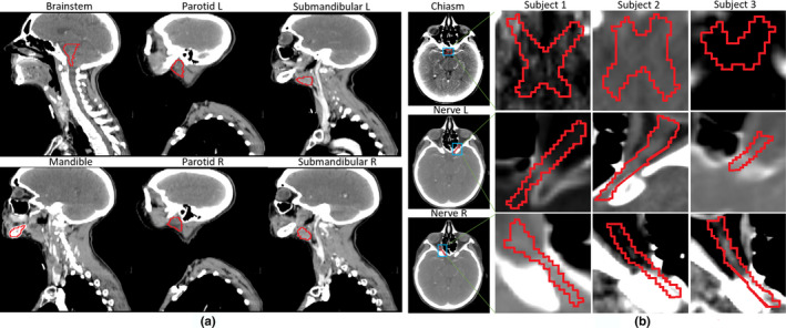
Examples of both large and small structures/tissues in the head and neck CT images of the Challenge. In (a), large tissues, including brainstem, mandible, parotid L/R, and submandibular L/R, are shown. In (b), the high intersubject variability in the small tissues and their low boundary contrast can be observed for both the chiasm and the left/right optic nerve. [Color figure can be viewed at wileyonlinelibrary.com]

To address the obstacles in the segmentation of the head and neck CT images, many prior knowledge‐based approaches have been developed in the last decades. These segmentation approaches mainly fall into three categories.

1. Atlas‐based methods: The multiatlas‐based segmentation (MABS) methods use a database of atlas images with manually segmented Regions Of Interest (ROIs). Optimal atlases are selected from the database, and registered to the target image under segmentation. The ROIs of the registered atlases are then transferred to the target image to produce the segmentation result.⁶ Several variants of MABS have been proposed, including the use of the average patient anatomy,⁷ the improved atlas selection strategies,^{7, 8, 9} and the voting strategies^{10, 11} (i.e., by assigning dynamic weights to ensemble all the available individual atlases for better fusion of the target ROIs). If a database of atlases is available, multiple segmentations from the atlases can be propagated and fused to complete the segmentation of the subject. The voting step, which is a practical way to fuse all atlases, is thus of great importance to multiatlas segmentation. For example, Han et al.² have developed a fully automated atlas‐based method for head and neck CT image segmentation using a novel hierarchical atlas registration approach.

2. Statistical shape/appearance‐based methods: These segmentation methods based on statistical shape models or statistical appearance models typically produce the closed surfaces that can well‐preserve anatomical topologies, since the final segmentation results are constrained by the statistical models. To this end, the variation in shapes and/or appearances of the ROIs under consideration needs to be encoded from a set of training images in advance. The variation in the anatomies can be represented by using landmarks, surface meshes, or appearance statistics of voxel intensities. Qazi et al.¹² present a fully automated hybrid approach for combining the deformable registration with the statistical shape/appearance‐based approach to accurately segment both normal and target tissues from the head and neck CT images. Fritscher et al.¹³ utilize the atlas‐based segmentation and label fusion to initialize a segmentation pipeline that is designed based on statistical appearance models and geodesic active contours.

3. Classification‐based methods: Voxel‐wise classification has been employed in the context of image segmentation for automatically detecting and classifying different types of tissues. Often, classification methods train the classifiers (e.g., Support Vector Machine and Random Forest) from the features extracted from the neighborhood of each individual voxel under segmentation. The classifiers are then used for voxel‐wise tissue classification/segmentation, without enforcing any shape constraint on the segmented tissues. Srhoj‐Egekher et al.¹⁴ employ a local tissue‐specific supervised voxel classification to segment the ROI. Yang et al.¹⁵ utilize Support Vector Machine to differentiate the parotid by statistically matching multiple texture features. Ma et al.¹⁶ utilize a nonlinear classification forest to automatically fuse both image and label information for brain segmentation. Qian et al.¹⁷ employ a random forest technique to effectively integrate features from multisource images with an auto‐context strategy.

Deep learning has also been perceived as an efficient tool for supervised learning. In particular, Convolutional Neural Network (CNN) has been developed into a typical deep learning method.¹⁸ Compared with the classical machine learning algorithms, CNN does not require hand‐crafted features for classification. Instead, the network is capable of learning the best features during the training process. CNN has been applied to a variety of biomedical imaging problems.¹⁹ In particular, Ciresan et al.²⁰ present the first GPU implementation of a 2D‐CNN for segmentation of neural membranes.

In this work, we will present a deep learning‐based solution to tackle the segmentation of the head and neck CT images. In particular, we will focus on the very challenging task of segmenting small tissues (i.e., both the chiasm and the left/right optic nerves). To this end, we build several 3D‐CNNs, respectively, for different tissues to determine tissue labels of individual voxels according to their surrounding 3D image patches. Importantly, the CNNs are trained and tested with multi‐scale patches, such that large patch helps locate the tissue while small patch contributes to precise labeling of each voxel under consideration. Moreover, we observe that the segmentation tasks of individual small tissues should better be jointly considered, as chiasm and optic nerves are closely related in terms of the physiological and anatomical perspective. Therefore, we interleave and cascade the CNNs for individual tissues, such that the tentative segmentation result of a certain tissue can be used to help refine (a) the segmentation of other tissue as well as (b) the segmentation of itself. This interleaving strategy leads to a complex network of CNNs, where all regions of interest (ROIs) can be automatically segmented. The performance of our proposed method was demonstrated upon the Challenge data. In particular, the DC scores rise to 0.58 for optic chiasm and 0.71 for optic nerves, which are significantly higher than the best scores (0.38 and 0.68) reported in the literature.²¹

Joint segmentation strategy has been used in medical images. Among the methods leveraging context information, the auto‐context model (ACM) has been shown highly effective.²² Gao, Liao, Shen²³ have proposed a novel prostate segmentation method based on ACM. Kim, Wu, Li, Wang, Son, Cho, Shen²⁴ have presented a learning‐based algorithm for automatic segmentation by taking advantages of the MABS and the ACM. Another joint segmentation way is multitask strategy. Gao, Shao, Lian, Wang, Chen, Shen²⁵ have proposed a multitask random forest to learn the displacement regressor jointly with the organ classifier. Wu, Wang, Lian, Shen²⁶ have presented a unified approach to estimate the respiratory lung motion with two iterative steps including spatiotemporal registration and super‐resolution strategy. Regarding our work, the major contributions include (a) Our proposed framework focuses on how to combine context information of different tissues rather than a single tissue. (b) Based on the anatomical prior knowledge, the interleaved scheme was carefully designed, such that both tissues can help segment each other. (c) The multiscale strategy is effective to be adopted for segmenting small tissues in head and neck CT images

The rest of the paper is organized as follows. In Section 2, we describe our interleaved 3D‐CNNs for joint segmentation of small tissues in the head and neck CT images. Then, in Section 3, we conduct a series of experiments to comprehensively validate our novel strategies and compare our method with the state‐of‐the‐art methods. Finally, discussions are presented in Sections 4 with our conclusions in Section 5.

2. Materials and methods

All images were processed and adopted in MABS for the rough yet robust localization of the ROIs first. Then, the CNNs are trained to take into account the patch appearance information of each voxel, and compute the probabilities of the voxel belonging to the individual tissue labels. Note that the CNNs, for each respective tissue, utilize multiscale patch appearance information of the voxels. Moreover, we interleave multiple 3D‐CNNs such that (a) the tentative segmentation result of a certain tissue can be used to help segmentation of other tissues as well as (b) the previous tentative segmentation result can be used to refine the current segmentation of same tissue.

2.A. Dataset of the Challenge

We validate our method on the Challenge dataset in this work, which was provided and maintained by Dr. Gregory C Sharp (Harvard Medical School – MGH, Boston, MA, USA). There are 48 patient CT images, together with manual segmentations of parotid glands (both left and right), brainstem, optic chiasm, optic nerves (both left and right), mandible, and submandibular glands (both left and right), as well as manual identification of bony landmarks. The image size is 512 × 512 × 120 in voxel, and the spacing is 1.12 × 1.12 × 3 mm.³ The primary objective of this dataset is to establish a benchmark for unbiased evaluation of automatic segmentation methods.

The Challenge dataset splits into four subsets:

1. Images and labels of 0522c001–0522c0328 (25 subjects in total) were provided as the training set;

2. Images and labels of 0522c329–0522c0479 (eight subjects in total) were provided as an additional training set;

3. Images of 0522c555–0522c0746 (10 subjects in total) were provided as the offsite test set for the challenge;

4. Images of 0522c0788–0522c0878 (five subjects in total) were used as the onsite test set.

In this paper, both the training and the additional training sets are utilized (totally 33 = 25 + 8 images) to build the network of interleaved 3D‐CNNs, and then test its performance with both the offsite and onsite sets (totally 15 = 10 + 5 images). The protocol above is consistent with all methods under comparison.

2.B. Image preprocessing

To initiate the segmentation of the target CT image, we have a set of training images with manually labeled ROIs. In the beginning of the preprocessing, an HU window of [−200, 200] is adopted to threshold all images. In this way, the soft tissue regions under consideration (i.e., chiasm and optic nerves) can be clearly observable to human eyes. Considering that the ROIs are relatively small in volumes, the MABS method is adopted to locate the ROIs roughly. In particular, we adopt normalized mutual information as a similarity metric for guiding the registration of all training atlas images to the target image. The registration consists of affine transformation and B‐Spline‐based nonlinear deformation. The warped ROIs of the training atlas images are fused by following the strategy proposed by Sabuncu et al.¹¹ The above MABS implementation is attained by the open‐source toolkit in Zaffino et al.²⁷ The probability map output by MABS is dilated by the radius 6 × 6 × 1 in voxels. In the subsequent CNN‐based segmentation, we will only handle the voxels located in the above dilated areas.

2.C. Multiscale 3D‐CNN for voxel‐wise classification

Convolutional neural network has been widely used for image segmentation. CNN often consists of multiple layers. In particular, each layer involves either linear or nonlinear operators, where the parameters of operators can be learned jointly for all layers and in an end‐to‐end manner. Due to its outstanding performance, CNN has become a dominant approach for many computer vision studies. In particular, VGG network²⁸ adopts very small (e.g., 3 × 3 in 2D) convolutional filters in its layers. And it can push to very deep layers and improve the performances of CNN significantly. Inspired by the excellent performance of VGG network, small convolutional filters are adopted in our 3D‐CNN for segmentation of the head and neck CT images.

The architecture of the 3D‐CNN network is shown in Fig. 2(a). The input data (i.e., image patch) flow into two convolutional layers, followed by a pooling layer, and ends with an additional convolutional layer. Finally, in the fully connected layer of 256 neurons, all feature representations are concatenated and produced by the last convolutional layer for computing the probability of assigning a specific tissue label to the center voxel of the patch under consideration. The Batch Normalization (BN) technology is adopted before each convolutional layer.²⁹ Batch Normalization allows us to use much higher learning rates and to be less careful about initialization. It also acts as a regularizer, in some cases eliminating the need for Dropout. The REctified Linear Unit (RELU) activation function³⁰ is also applied in the convolutional layers; the use of the rectifier as a nonlinearity has been shown to enable the training of deep supervised neural networks without requiring unsupervised pretraining. To improve the robustness, the dropout strategy³¹ is further adopted in both convolutional layers and fully connected layer as it can greatly improve the performance of neural networks as well as reducing the influence of overfitting.

Figure 2.

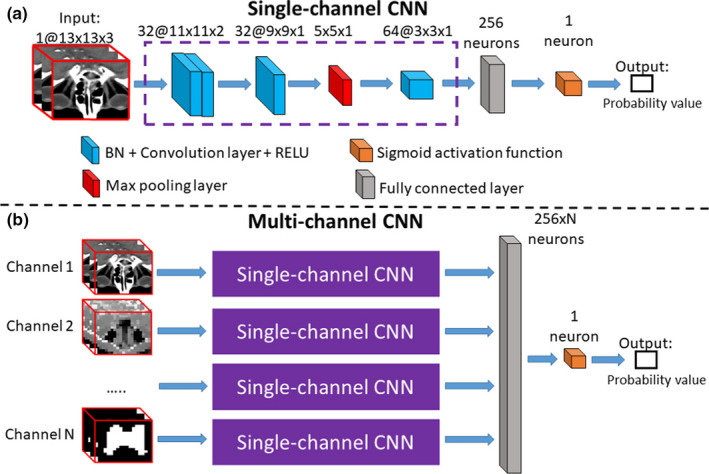
Illustration of single‐channel CNN and multichannel CNN. The single‐channel CNN in (a) computes the probability of assigning a specific tissue label to the center voxel of the input 3D patch. The single‐channel CNN consists of three convolutional layers, one pooling layer, and one fully connected layer. The numbers of the filters, as well as the support of each filter, are marked on the top of each layer. In (b), a multichannel CNN is derived from several single‐channel CNNs, to account for the multichannel input patches in our proposed framework. The multichannel information includes multiscale image patch from CT and the probability map patch derived from previous iteration. The probability map generated by other CNNs can be treated as an input to the multichannel CNN here, such that the segmentation of all ROIs can be solved jointly and iteratively. [Color figure can be viewed at wileyonlinelibrary.com]

The network is trained using the Theano toolkit.³² Log loss is adopted in the logistic regression as our loss function, which is minimized by Adam.³³ The weights in the networks are initialized randomly with a Gaussian distribution (using the mean 0 and the standard deviation 1 × 10⁻⁴).¹⁸ During the training, the weights are updated by Adam with a learning rate of 0.001. The number of the epochs is tuned on a validation set randomly selected from the training patches. If the validation accuracy does not increase in five consecutive epochs, the training will be terminated. In our experiments, the training process usually converges after 11 epochs for all tissues. Thirty‐three samples are employed for training and validation. Patches are randomly sampled within the dilated areas, which is described in Section 2.B. In every epoch, the numbers of the patches are 62437, 89956, and 97427, respectively, for Chiasm, Nerve L, and Nerve R. For each training or validation patch, the tissue label for the center voxel is provided. With a single Nvidia Titan X GPU, it takes 4 h to complete the training upon all ROIs. In the testing, we spend 30 s segmenting the three tissues from each subject. Note that the MABS initialization time for each subject needs 15 min.

The above CNN is able to handle a single input channel of 3D patch only. The size of 1@13 × 3 × 3 block is input to our single‐channel network. The first and second layers are the kernel of 32@3 × 3 × 2 with stride of 1 × 1 × 1 convolution operation. After these two convolution layers, the size of block becomes 32@9 × 9 × 1. Then, the kernel of 2 × 2 × 1 with 2 × 2 × 1 stride pooling layer is utilized. For the odd number of blocks, we choose to zero‐pad the image. So, the block is padded to the size of 32@10 × 10 × 1. After these pooling operations, the output shape is 32@5 × 5 × 1. In a similar way, the kernel of 64@3 × 3 × 2 is adopted with stride of 1 × 1 × 1 convolution layer, and then obtain 64@3 × 3 × 1 blocks. In addition, the block is flattened into one dimension, by the utilizing a fully connected layer with 256 neurons to “fully” connect each of neurons flattened from 64@3 × 3 × 1 blocks. Finally, we set a sigmoid activation layer to solve the binary classification problem. The layer‐by‐layer parameters of the single‐channel CNN are listed in Table 1.

Table 1.

The layer‐by‐layer parameters of the single‐channel CNN

Layer	Filter size/stride	Filter number
Convolution	3 × 3 × 2/1 × 1 × 1	32
Convolution	3 × 3 × 2/1 × 1 × 1	32
Max pooling	2 × 2 × 1/2 × 2 × 1	32
Convolution	3 × 3 × 1/1 × 1 × 1	64

Multiscale patches are extracted to represent the same center voxel. To this end, we extend the above single‐channel 3D‐CNN to the multichannel 3D‐CNN, where each channel corresponds to the input patches of a specific scale. With a network of multichannel 3D‐CNNs for each ROI, we can classify the voxels according to their multiscale patch representations, that is, computing the probabilities of each voxel belonging to different tissues labels. The architecture of the multichannel CNN is shown in Fig. 2(b). The multiscale patches flow into the respective single‐channel CNNs, and then all the information is fused in the final fully connected layer. Moreover, we note that the multichannel inputs allow not only the multiscale image patches but also the patches of tentative segmentation results (e.g., the last input channel in Fig. 2(b), corresponding to the tentative segmentation map). In this way, the multichannel 3D‐CNN facilitates interleaving multiple CNNs for joint tissue segmentation, which will be detailed later.

We argue that the image patch of large scale provides context information to locate the voxel with respect to the nearby structures in the image. The patch of small scale then provides detailed appearance information for precise labeling of the voxel, that is, determining whether the voxel under consideration is exactly on the edge of the ROI. Our experiments reveal that, by combining the patches of multiple scales, the voxel‐wise classification tends to be more robust and accurate in segmenting small tissues in the head and neck CT images. Detailed results are shown in Section 3.A. Empirically, 13 × 13 × 3 (in voxel) is adopted as the size of the 3D patches for all input channels, while the resolution of the patch varies for different scales. The original resolution of CT images is 1.12 × 1.12 × 3 mm³. Then, in our implementation, two 3D patches are adopted with the voxel spacing of 1.12 × 1.12 × 3 mm³ and 4.48 × 4.48 × 3 mm³, respectively, to characterize the appearance of the center voxel. The choices of the patches as well as parameters will be evaluated in the experimental section.

2.D. Interleaved CNNs for joint tissue segmentation

We focus on the segmentation of small chiasm and optic nerves in the head and neck CT images in this work. An example of these tissues is shown in Fig. 3, from which we can observe the complex anatomical relationship among the ROIs. That is, the context information of the optic nerve is very important for the segmentation of the chiasm in expert's delineations. We also find that, with available chiasm segmentation, better optic nerve segmentation can be achieved. To this end, we propose to interleave the multichannel 3D‐CNNs for joint segmentation of chiasm and optic nerves.

Figure 3.

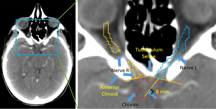
The anatomical relationship of the chiasm and the left/right optic nerves is highly coupled. The optic nerves are contoured up to the optic chiasm. In manual delineation, experts locate the chiasm with a line between the anterior clinoid and the tuberculum sellae. Then, the boundary between the optic nerve and the chiasm is drawn perpendicular to the center of the optic nerve. [Color figure can be viewed at wileyonlinelibrary.com]

To segment multiple ROIs jointly, a set of CNNs are trained, each corresponding to a specific ROI. In this way, we are able to specially optimize each CNN for the corresponding ROI, and also avoid the imbalanced numbers of training patches due to the sizes of individual ROIs. The proposed framework then interleaves the trained CNNs for joint tissue segmentation as shown in Fig. 4. Initially, we input multiscale 3D patches (of the fixed size 13 × 13 × 3, yet with the resolutions of 1.12 × 1.12 × 3 mm³ and 4.48 × 4.48 ×  3 mm³, respectively) to the first iteration of the network. The multichannel CNNs produce the probability maps to segment the ROIs independently. Then, the max strategy is adopted to determine the maximum segmentation probability from all tentative CNN outputs for a given voxel. A patch can be extracted from the aforementioned probability map, and it incorporates the context information of the segmentation of all nearby structures. The probability patch, which characterize the context information generated in the early iteration for the center voxel, is then inputted to the subsequent iteration of the network (i.e., alongside “channel N” in Fig. 2(b)). After reaching the last iteration, we can acquire three probability maps corresponding to the chiasm and the left/right nerves from respective CNNs. The resulted probability maps have been refined gradually throughout the network of the interleaved CNNs. Note that the probability maps paths are independent to each other including the CT image patch path. If there is a probability map added as input, there would a single‐channel CNN path corresponding to it. The multichannel CNN is trained as a whole network. To be specific, each separate single‐channel CNN in the multichannel CNN has its own parameter.

Figure 4.

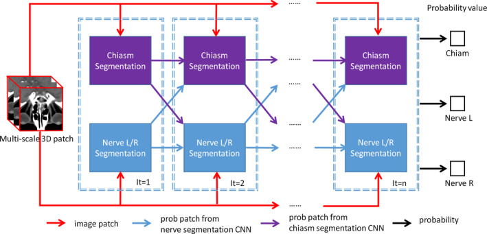
A network of the interleaved 3D‐CNNs for joint segmentation of both chiasm and optic nerves. Multiscale patches for the center voxel are used as the input, while the output reveals the probabilities of the center voxel belonging to different tissues. The “segmentation” blocks correspond to the individual 3D‐CNNs, which are interleaved and cascaded to derive the complex segmentation network. [Color figure can be viewed at wileyonlinelibrary.com]

2.E. Performance evaluation and validation

To quantitatively evaluate the performances of the automatic segmentation method, DC and the undirected 95% Hausdorff Distance (95HD)³⁴ are utilized as the metrics.⁴ All the metrics are produced by Plastimatch³⁵ for fair comparison with results in the challenge. The score of DC is defined as follows:

$$\mathrm{DC}=\frac{2\left|A\cap B\right|}{\left|A\right|+\left|B\right|}$$ (1)

where $A$ and $B$ denote the two delineated regions, respectively, and $|·|$ computes the volume of each specified region.

To implement 95HD, we first define the directed Hausdorff distance. Suppose that $X$ and $Y$ are two‐point sets, and $d\left(x,y\right)$ is the Euler distance between the points $x\in X$ and $y\in Y$. We have

$$\overrightarrow{d}\left(x,y\right)=\underset{x\in X}{max}\underset{y\in Y}{min}d\left(x,y\right)$$ (2)

The undirected Hausdorff distance is the maximum of the two directed Hausdorff measures:

$$d_H(\mathrm{x},\mathrm{y})=\text{max}(\overrightarrow{d}\left(x,y\right),\overrightarrow{d}\left(y,x\right))$$ (3)

The directed percent Hausdorff measure, for a percentile $r$, is the $r$th percentile distance over all distances from points in X to their closest point in Y. For example, the directed 95% Hausdorff distance is the distance of a point in X to its closest point in Y, which is greater or equal to exactly 95% of distances of the other points in X. Mathematically, by denoting the $r$‐the percentile as $K_r$, the directed 95% Hausdorff distance can given as:

$${\overrightarrow{d}}_{H,r}\left(x,y\right)=K_r\left(\underset{y\in Y}{min}d\left(x,y\right)\right),\forall xX$$ (4)

The (undirected) percent Hausdorff measure is defined as

$$d_{H,r}(\mathrm{x},\mathrm{y})=\frac{{\overrightarrow{d}}_{H,r}\left(x,y\right)+,{\overrightarrow{d}}_{H,r}\left(y,x\right)}{2}$$ (5)

There are several strategies in our method requiring quantitative validation. Multiscale patch representations are adopted for individual voxels in CNNs. To verify the contribution and evaluate the optimal configuration of the multiscale strategy, we conduct the following comparisons and report the results in Section 3.A.

• 1‐scale: In “1‐scale”, the single‐scale image patch is extracted and allow only a single input channel to the network of CNNs. The size of the patch is 13 × 13 × 3, and the spatial resolution of the patch is 1.12 × 1.12 × 3 mm³, which is equal to the resolution of the original CT image.

• 2‐scale: In addition to the image patch used in “1‐scale”, we add a second patch of larger scale. In particular, both patches are fixed to the size 13 × 13 × 3 for easy implementation of the multichannel CNNs. The spatial resolutions of the two patches are 1.12 × 1.12 × 3 mm³ and 4.48 × 4.48 × 3 mm³, respectively. Note that “2‐scale” is selected as the recommended configuration of our method according to the subsequent experimental results.

• 3‐scale: After determining the optimal configurations of “2‐scale”, we add a third scale of image patch to describe each voxel. In this way, we have three patches, with the respective spatial resolutions 1.12 × 1.12 × 3 mm³, 3.36 × 3.36 × 3 mm³, and 4.48 × 4.48 × 3 mm³, to characterize each voxel.

The joint segmentation strategy is adopted, by interleaving CNNs, to handle the three small ROIs in the head and neck CT images. That is, the context information of optic nerves and their tentative segmentation results are very important for the segmentation of chiasm, and vice versa. We conduct experiments to quantitatively validate the contributions of the joint segmentation strategy. For each ROI, our strategy allows its tentative segmentation to help improve the segmentation results of its neighboring ROIs as well as itself. To this end, we isolate the contributions and conduct the subsequent comparisons with results in Section 3.B.

• Strategy‐1 (S1): This strategy means that each of the three ROIs refines its segmentation result by using just its own context information, that is, in an auto‐context way.^{22, 36} Specifically, given a certain ROI, two CNNs are cascaded, such that the probability map outputted by the first CNN can be used as an input channel to the second CNN. In particular, the probability patch of the size 13 × 13 × 3 and the resolution 1.12 × 1.12 ×  3 mm³ is extracted.

• Strategy‐2 (S2): In manual delineation, the optic nerves provide an important reference to localize the chiasm. Therefore, one may assume that the chiasm contributes little to the segmentation of the optic nerves. To this end, in S2, we disable the information flow from the chiasm‐specific CNN to the CNNs that focus on the segmentation of the optic nerves. The patches extracted from the probability maps of the chiasm are at the resolution of 3.36 × 3.36 × 3 mm³, while the patches for the probability maps of the optic nerves are of 1.12 × 1.12 × 3 mm³.

• Strategy‐3 (S3): The assumption of this strategy is that all three ROIs can benefit each other. We set the respective optimal probability patch sizes for three tissues by exhaustive parameter searching. The S3 strategy is equivalent to our proposed joint segmentation in this work, except that only two iterations are conducted with the patch resolution of 3.36 × 3.36 × 3 mm³ for all the tissues.

2.F. Summary

We propose to interleave multiple 3D‐CNNs for joint segmentation of small tissues (i.e., chiasm and the left/right optic nerves) in the head and neck CT images. First, three CNNs are built, corresponding to three different scale patches, for each ROI. Next, a max probability map is computed by integrating the outputs of those three CNNs, and can be used to extract the probability patch for providing additional context information of each voxel. The probability patch extracted from early CNNs, as well as multiscale image patch, are interleaved and input to the subsequent CNNs. This interleaving procedure continues and finally yields a complex network of CNNs, as shown in Fig. 4, for accurate segmentations of all ROIs jointly.

3. Results

3.A. Contribution of the multiscale patches

Note that the optimal scales/sizes of the above comparisons are determined by exhaustive search of parameters. In order to show the importance of the multiscale patch description, the proposed network of interleaved 3D‐CNNs is reduced to the minimum. That is, three multichannel CNNs are trained (without any interleaving) to conduct independent segmentation for three ROIs. The multichannel inputs are the same multiscale patches as mentioned above.

We report the comparison results in Fig. 5. Note that the higher the better for DCs. While the lower the better for 95HD when used to measure the effect of image segmentation. The multiscale strategy proves to be effective, as both 2‐scale and 3‐scale yield higher DC scores and lower 95HD scores than 1‐scale. In particular, we note that the 2‐scale configuration, with the patches of the spatial resolutions 1.12 × 1.12 × 3 mm³ and 4.48 × 4.48 × 3 mm³, is the best for multiscale patch‐based segmentation in the Challenge dataset. Comparing 1‐scale and 2‐scale, the mean DC score is increased from 0.32 to 0.47 for chiasm, from 0.55 to 0.63 for nerve L, and from 0.55 to 0.61 for nerve R. The mean 95HD score is decreased from 5.4 to 4.0 mm for chiasm, from 3.8 to 3.0 mm for nerve L, and from 3.9 to 3.3 mm for nerve R. Compared to 3‐scale, 2‐scale is in general better (except for the right optic nerve), partially due to the complexity in modeling the CNNs when using too many input channels in 3‐scale. Accordingly, 2‐scale and its configuration are adopted in the subsequent experiments. The DC scores are significantly different between 1‐scale and 2‐scale (with P‐value 0.014 in paired t tests for chiasm; and P‐value 0.008 in paired t tests for nerve L). The 95HD scores are significantly different between 1‐scale and 2‐scale (with P‐value 0.008 in paired t tests for chiasm; and P‐value 0.05 in paired t tests for nerve R).

Figure 5.

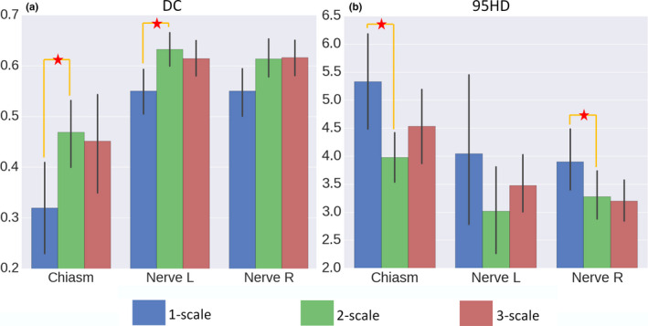
The DC (a) and 95HD (b) scores for 1‐, 2‐, and 3‐scale configurations. The multiscale strategy proves to be effective, as both 2‐scale and 3‐scale yield better scores than 1‐scale. In particular, we note that the 2‐scale configuration, with the patches of the spatial resolutions 1.12 × 1.12 × 3 mm³ and 4.48 × 4.48 × 3 mm³, is the best for the Challenge dataset. The asterisks denote statistical significance (i.e., P < 0.05 in t tests). [Color figure can be viewed at wileyonlinelibrary.com]

3.B. Contribution of the joint segmentation strategy

We compare the three joint segmentation strategies and report the results in Fig. 6. The S2/S3 strategy proves to be effective, as both S2 and S3 yield higher DC scores and lower 95HD scores than S1. In particular, we note that the S3 strategy is the optimal configuration for joint segmentation in the Challenge dataset. That is, the chiasm and the optic nerves should contribute mutually for their better segmentations. Comparing S1 and S3, the mean DC score is increased from 0.50 to 0.56 for chiasm, from 0.68 to 0.70 for nerve L, and from 0.65 to 0.68 for nerve R. The mean 95HD score is decreased from 3.7 to 3.5 mm for chiasm, from 2.9 to 2.4 mm for nerve L, and from 2.8 to 2.2 mm for nerve R. Similar conclusion can also be achieved except for 95HD of chiasm.

Figure 6.

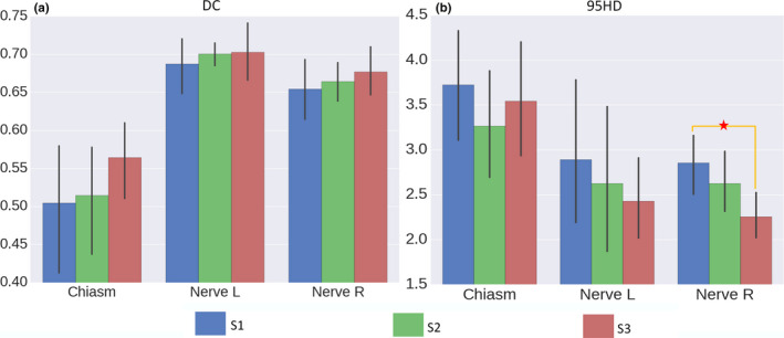
The DC (a) and the 95HD (b) scores for S1, S2, and S3. The S2/S3 strategy proves to be effective, as both S2 and S3 yield higher DC scores and lower 95HD scores than S1. The proposed joint segmentation strategy (S3) proves to be more effective than S2, as better scores can be achieved. The asterisks denote statistical significance (i.e., P < 0.05 in t tests). [Color figure can be viewed at wileyonlinelibrary.com]

3.C. Performance of our method

Starting with S3, we cascade more 3D‐CNNs and derive the complex network of the interleaved 3D‐CNNs as proposed in this paper. The performance of joint segmentation, with respect to the increasing number of iterations, is reported in Fig. 7. In this experiment, particularly, we adopt the optimal image size/resolution configurations determined early. Note that, in the 1st iteration, no tentative segmentation probability map is available. The results in Fig. 7 show that using the 4th iteration could have better DC or 95HD scores than using fewer iterations. Comparing the 4th and the 2nd iterations, the mean DC score is increased from 0.55 to 0.56 for chiasm, from 0.70 to 0.72 for nerve L, and from 0.68 to 0.70 for nerve R. The mean 95HD score is decreased from 3.5 to 3.0 mm for chiasm, from 2.5 to 2.3 mm for nerve L, and from 2.8 to 2.2 mm for nerve R. The observation confirms the effectiveness of interleaving multiple CNNs for small tissue segmentation in the Challenge dataset.

Figure 7.

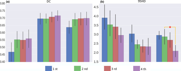
The DC and 95HD scores with respect to the increasing number of iterations, as more 3D‐CNNs are interleaved for joint segmentation of small tissues in the head and neck CT images. The 4th iteration strategy proves to be effective with better DC or 95HD score than using fewer iterations. The observation confirms the effectiveness of interleaving multiple CNNs for small tissue segmentation in the Challenge dataset. The asterisks denote statistical significance (i.e., P < 0.05 in t tests). [Color figure can be viewed at wileyonlinelibrary.com]

Finally, we show the visual comparisons of the segmentation results of S1 (with the traditional auto‐context strategy) and S3 (with our proposed joint segmentation strategy) in Fig. 8. All of the results are produced with four iterations as in Fig. 4. For chiasm, S1 results in oversegmentation in the second slice, while the proposed S3 strategy can still detect the correct slice by using the context information of optic nerves. Similar observation can also be acquired from the results of the left and the right optic nerves, as our joint segmentation strategy can produce results that fit the ground truth better. In conclusion, our joint segmentation strategy has improved the segmentation accuracy, especially when compared to the conventional auto‐context strategy (S1).

Figure 8.

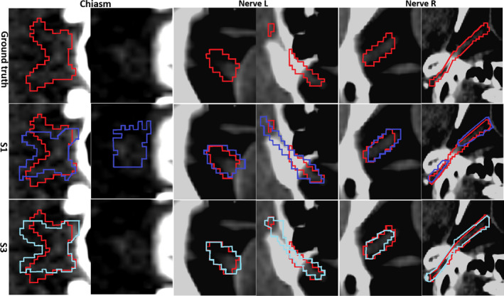
Visualization of the segmentation results of three ROIs. Red denotes for the ground truth, purple for S1 segmentation results, and blue for S3 results. All results are produced with four iterations of the complex network of interleaved 3D‐CNNs. Two consecutive slices are provided for each ROI. Our joint segmentation strategy (marked by “S3”) achieves the best performance.

3.D. Comparison with state‐of‐the‐art methods

The Challenge datasets provides a platform to compare many methods quantitatively. In particular, we compare our proposed method with state‐of‐the‐art methods, including their reported performances. The competing methods in the Challenge are summarized as follows.⁴

• VU (fully automatic):³⁷ This multiatlas approach registers patient images with the atlases at the global level, followed by the correlation‐based label fusion to determine the label locally.

• IM (fully automatic):²¹ This method builds the Active Appearance Models (AAMs) from manually segmented images. High‐quality anatomical correspondences for the models are generated using group‐wise registration. The models are then applied to segmenting individual ROIs in the CT images. The method ranks first in the Challenge.

• UB (semi‐automatic):³⁸ This method obtains an initial segmentation for the considered ROIs, and then refines the result with the Active Shape Model (ASM). The method ranks second in the Challenge. Note that this method is semi‐automatic. That is, for the initial registration, a small number of landmarks should be manually designated.

For comparison purpose, Tables 2 and 3 list the average DC and 95HD scores reported in the Challenge paper. Note that the comparisons follow the same training/testing protocol. The bold italic values are the best score for each column.

Table 2.

Comparisons of DC scores for all the competing methods

	Chiasm	Nerve L	Nerve R	Nerve avg
VU	0.38 ± 0.12	0.65 ± 0.11	0.61 ± 0.09	0.63 ± 0.10
IM	0.38	–	–	0.68
UB	0.55 ± 0.16	0.59 ± 0.07	0.51 ± 0.08	0.55 ± 0.07
Ours	0.58 ± 0.17	0.72 ± 0.08	0.70 ± 0.09	0.71 ± 0.08

Table 3.

Comparisons of 95HD scores for all the competing methods (unit: mm)

	Chiasm	Nerve L	Nerve R	Nerve avg
VU	4.13 ± 0.82	2.76 ± 0.70	3.15 ± 1.27	2.96 ± 0.96
IM	3.48	–	–	2.48
UB	2.78 ± 0.79	3.23 ± 0.99	3.20 ± 1.08	3.22 ± 1.04
Ours	2.81 ± 1.56	2.33 ± 0.84	2.13 ± 0.96	2.23 ± 0.9

According to Tables 2 and 3, our proposed method outperforms all other methods in the Challenge, with the highest mean DC score for each ROI. Especially, compared with the Challenge winner of IM, our segmentation results are significantly better in chiasm, with a relatively small margin over L/R nerves. For 95HD results, only the chiasm result of our method is slightly worse than UB, while our method is still much better in all other comparisons. The DC scores are significantly different between VU and our method in all tissues, as well as between UB and our method in L nerve. The 95HD scores are significantly different between VU and our method in L nerve, as well as between UB and our method in L nerve. We are unable to conduct statistical analysis against IM due to the limited data disclosure. Considering UB is the semi‐automatic method in this Challenge, our (automatic) method can be regarded as a more accurate and flexible method.

4. Discussion

We have presented a method for automatic segmentation of small tissues in the head and neck CT images, and evaluated its performance with the MICCAI 2015 Challenge dataset. Different from previous techniques, our proposed method uses a series of deep neural networks to perform the entire segmentation work. In particular, our method interleaves multiple 3D‐CNNs for joint segmentation of all tissues under consideration. For the tissues including chiasm and optic nerves, they are small and poorly visible in the CT images. However, our method shows its capability of labeling those small tissues better than the state‐of‐the‐art methods in general. We note that our proposed framework focuses on how to combine different tissues and their context information to improve the segmentation accuracy. There exists a large space to improve our proposed architecture for the network of interleaved 3D‐CNNs, as well as to tune the parameters, both of which will be part of our future work. For our initial algorithm, MABS is a time‐consuming initialization method. It would be also interesting to explore whether a simpler and more accurate method can be developed to locate the ROIs.

The Challenge data present similar appearance characteristics in both training and testing. However, we manually check the ground truth delineation case by case, and reveal several outlier samples for testing. The variation in the manual delineation can be extremely high for small chiasm. In order to consistently define the boundary of the chiasm in manual delineation, experts are expected to locate it at a line between the anterior clinoid and the tuberculum sellae, and to include a short length of optic nerve within the chiasm. However, the rule above is not strictly followed for certain “outlier” samples. In general, the outliers in the Challenge dataset are 0522c0014, 0522c0149, 0522c0329, 0522c0455, 0522c0457, 0522c0659, 0522c0661, 0522c0667, and 0522c0746. An example (0533c0667) is shown in Fig. 9. Clearly, our method fails to achieve a good segmentation result, by generating a DC score of 0.36 only for the chiasm. There are some reasons for these results: (a) The relative positions of chiasm and optic nerves are not consistent with the guidance in the training data; (b) The shape and the position of optic nerves are deviating from the normal. To this end, we argue that a larger dataset is necessary for developing and evaluating a highly robust segmentation tool for small anatomical structures.

Figure 9.

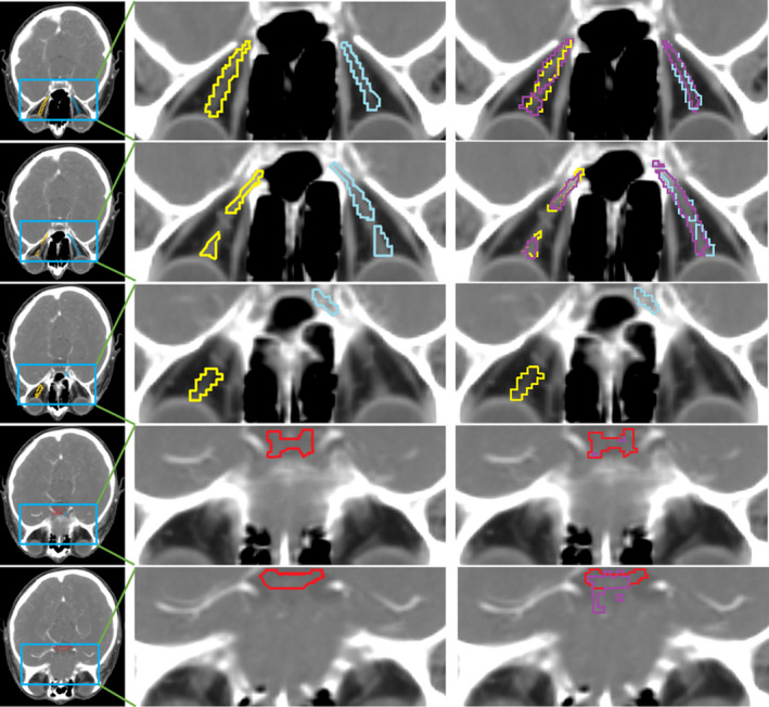
Visualization of an outlier sample (ID: 0533c0667). Red denotes the chiasm ground truth, yellow for nerve L ground truth, and blue for nerve R ground truth. Purple is for our segmentation results, which are overlaid on the right column only for visual comparison. From top to bottom are slice #100 to #104 of the sample. Our method yields a fragmentized segmentation result for this sample and gets the DC of only 0.36 for the chiasm.

Meanwhile, by eliminating the aforementioned outliers from testing, we further compare our method with UB. The DC scores of our method are 0.66 for chiasm, 0.75 for nerve L, and 0.71 for nerve R, while the scores of UB are 0.56 for chiasm, 0.63 for nerve L, and 0.65 for nerve R. The 95HD scores of our method are 2.69 for chiasm, 2.30 for nerve L, and 2.60 for nerve R, while the scores of UB are 2.79 for chiasm, 2.92 for nerve L, and 3.34 for nerve R. The margins become clearly wider and more statistically significant between our method and UB.

Table 4 is the average time cost for one testing subject. The bold italic value is the best score for column. According to this, our proposed method has a comparable time cost with all other methods in the Challenge, which are also based on MABS. Our method has large advantages, considering both performance and time cost.

Table 4.

Comparisons of time for all the competing methods (unit: min)

Method	Time
VU	20
IM	30
UB	12
Ours	15.5

Although we focus on segmenting small tissues in this work, our method can also handle large tissues well, including mandible, parotid, and brainstem in the Challenge dataset. In particular, we achieve the DC scores of 0.84 for brainstem, 0.81 for parotid L, 0.80 for parotid R, and 0.92 for mandible. The 95HD scores of 2.92 for brainstem, 3.93 for parotid L, 3.73 for parotid R, and 1.89 for mandible. These results are comparable to the winner methods in the challenge, that is, the DC scores of 0.88 for brainstem, 0.84 for parotid L, 0.84 for parotid R, and 0.92 for mandible, as well as the 95HD scores of 3.69 for brainstem, 5.94 for parotid L, 5.94 for parotid R, and 2.13 for mandible.

5. Conclusion

The primary contribution of our work is the use of interleaved 3D‐CNNs for joint segmentation of the small tissues in the head and neck CT images. Different from previous techniques, our proposed method uses a series of deep neural networks to perform the entire segmentation work. Our method has achieved better performance compared to the state‐of‐the‐art methods. Note that, although we focus on segmenting small tissues in this work, our method can still yield much better segmentation results than the state‐of‐the‐art methods on all relatively large tissues of the Challenge dataset. In conclusion, our method greatly improves the segmentation performance for the head and neck CT images.

Conflict of interest

The authors have no conflicts to disclose.

References

- 1. Jemal A, Bray F, Center MM, Ferlay J, Ward E, Forman D. Global cancer statistics. CA Cancer J Clin. 2011;61:69–90. [DOI] [PubMed] [Google Scholar]
- 2. Han X, Hoogeman MS, Levendag PC, et al. Atlas‐based auto‐segmentation of head and neck CT images. Paper presented at: International Conference on Medical Image Computing and Computer‐Assisted Intervention 2008. [DOI] [PubMed]
- 3. Berrino F, Gatta G, Group EW. Variation in survival of patients with head and neck cancer in Europe by the site of origin of the tumours. Eur J Cancer. 1998;34:2154–2161. [DOI] [PubMed] [Google Scholar]
- 4. Raudaschl PF, Zaffino P, Sharp GC, et al. Evaluation of segmentation methods on head and neck CT: auto‐segmentation challenge 2015. Med Phys. 2017;44:2020–2036. [DOI] [PubMed] [Google Scholar]
- 5. Sørensen T. A method of establishing groups of equal amplitude in plant sociology based on similarity of species and its application to analyses of the vegetation on Danish commons. Biol Skr. 1948;5:1–34. [Google Scholar]
- 6. Iglesias JE, Sabuncu MR. Multi‐atlas segmentation of biomedical images: a survey. Med Image Anal. 2015;24:205–219. [DOI] [PMC free article] [PubMed] [Google Scholar]
- 7. Commowick O, Warfield SK, Malandain G. Using Frankenstein's creature paradigm to build a patient specific atlas. Paper presented at: International Conference on Medical Image Computing and Computer‐Assisted Intervention 2009. [DOI] [PMC free article] [PubMed]
- 8. Rohlfing T, Brandt R, Menzel R, Maurer CR. Evaluation of atlas selection strategies for atlas‐based image segmentation with application to confocal microscopy images of bee brains. NeuroImage. 2004;21:1428–1442. [DOI] [PubMed] [Google Scholar]
- 9. Sanroma G, Wu G, Gao Y, Shen D. Learning to rank atlases for multiple‐atlas segmentation. IEEE Trans Med Imaging. 2014;33:1939–1953. [DOI] [PMC free article] [PubMed] [Google Scholar]
- 10. Hartmann SL, Parks MH, Martin PR, Dawant BM. Automatic 3‐D segmentation of internal structures of the head in MR images using a combination of similarity and free‐form transformations. II. Validation on severely atrophied brains. IEEE Trans Med Imaging. 1999;18:917–926. [DOI] [PubMed] [Google Scholar]
- 11. Sabuncu MR, Yeo BT, van Leemput K, Fischl B, Golland P. A generative model for image segmentation based on label fusion. IEEE Trans Med Imaging. 2010;29:1714–1729. [DOI] [PMC free article] [PubMed] [Google Scholar]
- 12. Qazi AA, Pekar V, Kim J, Xie J, Breen SL, Jaffray DA. Auto‐segmentation of normal and target structures in head and neck CT images: a feature‐driven model‐based approach. Med Phys. 2011;38:6160–6170. [DOI] [PubMed] [Google Scholar]
- 13. Fritscher KD, Peroni M, Zaffino P, Spadea MF, Schubert R, Sharp G. Automatic segmentation of head and neck CT images for radiotherapy treatment planning using multiple atlases, statistical appearance models, and geodesic active contours. Med Phys. 2014;41:051910. [DOI] [PMC free article] [PubMed] [Google Scholar]
- 14. Srhoj‐Egekher V, Benders M, Kersbergen KJ, Viergever MA, Isgum I. Automatic segmentation of neonatal brain MRI using atlas based segmentation and machine learning approach. MICCAI Grand Challenge: Neonatal Brain Segmentation; 2012:2012. [Google Scholar]
- 15. Yang X, Wu N, Cheng G, et al. Automated segmentation of the parotid gland based on atlas registration and machine learning: a longitudinal MRI study in head‐and‐neck radiation therapy. Int J Radiat Oncol Biol Phys. 2014;90:1225–1233. [DOI] [PMC free article] [PubMed] [Google Scholar]
- 16. Ma G, Gao Y, Wu G, Wu L, Shen D. Nonlocal atlas‐guided multi‐channel forest learning for human brain labeling. Med Phys. 2016;43:1003–1019. [DOI] [PMC free article] [PubMed] [Google Scholar]
- 17. Qian C, Wang L, Gao Y, et al. In vivo MRI based prostate cancer localization with random forests and auto‐context model. Comput Med Imaging Graph. 2016;52:44–57. [DOI] [PMC free article] [PubMed] [Google Scholar]
- 18. LeCun Y, Bottou L, Bengio Y, Haffner P. Gradient‐based learning applied to document recognition. Proc IEEE. 1998;86:2278–2324. [Google Scholar]
- 19. Shen D, Wu G, Suk H‐I. Deep learning in medical image analysis. Annu Rev Biomed Eng. 2017;19:221–248. [DOI] [PMC free article] [PubMed] [Google Scholar]
- 20. Ciresan D, Giusti A, Gambardella LM, Schmidhuber J. Deep neural networks segment neuronal membranes in electron microscopy images. Paper presented at: Advances in neural information processing systems 2012.
- 21. Mannion‐Haworth R, Bowes M, Ashman A, Guillard G, Brett A, Vincent G. Fully automatic segmentation of head and neck organs using active appearance models. 01 2016.
- 22. Huynh T, Gao Y, Kang J, et al. Estimating CT image from MRI data using structured random forest and auto‐context model. IEEE Trans Med Imaging. 2016;35:174–183. [DOI] [PMC free article] [PubMed] [Google Scholar]
- 23. Gao Y, Liao S, Shen D. Prostate segmentation by sparse representation based classification. Med Phys. 2012;39:6372–6387. [DOI] [PMC free article] [PubMed] [Google Scholar]
- 24. Kim M, Wu G, Li W, et al. Automatic hippocampus segmentation of 7.0 Tesla MR images by combining multiple atlases and auto‐context models. NeuroImage. 2013;83:335–345. [DOI] [PMC free article] [PubMed] [Google Scholar]
- 25. Gao Y, Shao Y, Lian J, Wang AZ, Chen RC, Shen D. Accurate segmentation of CT male pelvic organs via regression‐based deformable models and multi‐task random forests. IEEE Trans Med Imaging. 2016;35:1532–1543. [DOI] [PMC free article] [PubMed] [Google Scholar]
- 26. Wu G, Wang Q, Lian J, Shen D. Estimating the 4D respiratory lung motion by spatiotemporal registration and building super‐resolution image. Med Image Comput Comput Assist Interv. 2011;2011:532–539. [DOI] [PMC free article] [PubMed] [Google Scholar]
- 27. Zaffino P, Raudaschl P, Fritscher K, Sharp GC, Spadea MF. Technical Note: plastimatch mabs, an open source tool for automatic image segmentation. Med Phys. 2016;43:5155–5160. [DOI] [PubMed] [Google Scholar]
- 28. Simonyan K, Zisserman A. Very deep convolutional networks for large‐scale image recognition. arXiv preprint arXiv:1409.1556. 2014.
- 29. Ioffe S, Szegedy C. Batch normalization: Accelerating deep network training by reducing internal covariate shift. arXiv preprint arXiv:1502.03167. 2015.
- 30. Nair V, Hinton GE. Rectified linear units improve restricted boltzmann machines. Paper presented at: Proceedings of the 27th international conference on machine learning (ICML‐10) 2010.
- 31. Srivastava N, Hinton GE, Krizhevsky A, Sutskever I, Salakhutdinov R. Dropout: a simple way to prevent neural networks from overfitting. J Mach Learn Res. 2014;15:1929–1958. [Google Scholar]
- 32. Bergstra J, Breuleux O, Bastien F, et al. Theano: a CPU and GPU math compiler in Python. Paper presented at: Proc. 9th Python in Science Conf 2010.
- 33. Kingma D, Ba J. Adam: A method for stochastic optimization. arXiv preprint arXiv:1412.6980. 2014.
- 34. Dubuisson M‐P, Jain AK. A modified Hausdorff distance for object matching. Paper presented at: Pattern Recognition, 1994. Vol. 1‐Conference A: Computer Vision & Image Processing., Proceedings of the 12th IAPR International Conference on 1994.
- 35. Shackleford J, Shusharina N, Verberg J, et al. Plastimatch 1.6: current capabilities and future directions. Paper presented at: Proc. MICCAI 2012.
- 36. Tu Z, Bai X. Auto‐context and its application to high‐level vision tasks and 3d brain image segmentation. IEEE Trans Pattern Anal Mach Intell. 2010;32:1744–1757. [DOI] [PubMed] [Google Scholar]
- 37. Chen A, Dawant B. A multi‐atlas approach for the automatic segmentation of multiple structures in head and neck CT images. 02 2016.
- 38. Albrecht T, Gass T, Langguth C, Lüthi M. Multi atlas segmentation with active shape model refinement for multi‐organ segmentation in head and neck cancer radiotherapy planning. 12 2015.