Rotationally-invariant mapping of scalar and orientational metrics of neuronal microstructure with diffusion MRI

Abstract

We develop a general analytical and numerical framework for estimating intra- and extra-neurite water fractions and diffusion coefficients, as well as neurite orientational dispersion, in each imaging voxel. By employing a set of rotational invariants and their expansion in the powers of diffusion weighting, we analytically uncover the nontrivial topology of the parameter estimation landscape, showing that multiple branches of parameters describe the measurement almost equally well, with only one of them corresponding to the biophysical reality. A comprehensive acquisition shows that the branch choice varies across the brain. Our framework reveals hidden degeneracies in MRI parameter estimation for neuronal tissue, provides microstructural and orientational maps in the whole brain without constraints or priors, and connects modern biophysical modeling with clinical MRI.

1. Introduction and overview of results

Brownian motion of water molecules is strongly hindered by neurite walls (Beaulieu, 2002). Serendipitously, this sensitivity to tissue microstructure can be probed with NMR for diffusion times t ~ 1 − 1000 ms, corresponding to a diffusion length (rms molecular displacement) ℓ(t) ~ 1 − 100 μm commensurate with cell dimensions. The resulting diffusion MRI (dMRI) signal, acquired over a macroscopic imaging voxel, is an indirect but powerful probe into neuronal structure at the scale ℓ(t), 2–3 orders of magnitude below the MRI resolution.

The dMRI signal is generally anisotropic (Basser et al., 1994; Beaulieu, 2002; Jones, 2010), non-Gaussian (Le Bihan, 1995; Kroenke et al., 2004; Assaf et al., 2004; Kiselev and Il’yasov, 2007; Jespersen et al., 2007, 2010; Fieremans et al., 2011; Ferizi et al., 2015; Veraart et al., 2016b; Jensen et al., 2016), and time-dependent (Stanisz et al., 1997; Assaf and Cohen, 1998; Novikov et al., 2014; Fieremans et al., 2016). Description of this complex process simplifies at long times t ~ 100 ms, used in clinical dMRI, when ℓ(t) ~ 10 μm exceeds typical neurite diameters a ≲ 1 μm. In this regime, diffusion approaches its Gaussian limit separately in the intra- and extra-neurite spaces, Fig. 1. Biologically distinct hindrances lead to coarse-grained (Novikov et al., 2016) diffusion coefficients inside (D_a) and outside ( $D_e^{\Vert }$ and $D_e^{\perp }$) neurites within an elementary fiber fascicle; transverse diffusion ~ a²/t ≪ D_a inside neurites then becomes negligible (Kroenke et al., 2004). The dMRI signal (voxel-averaged diffusion propagator) is an ensemble average over contributions of individual fascicles within a voxel.

Figure 1. Standard Model of diffusion in neuronal tissue.

In the long time limit, elementary fiber segments (fascicles), consisting of intra- and extra-neurite compartments, are described by at least 4 independent parameters: f, D_a, $D_e^{\Vert }$ and $D_e^{\perp }$. Within a macroscopic imaging voxel, such segments contribute to the directional dMRI signal according to their ODF ℘(n̂). Due to its rich orientational content, the total number of parameters (10) characterizing a voxel is about 30 – 50.

Here we investigate in detail the general picture of anisotropic Gaussian compartments, Fig. 1, as an overarching “ Standard Model”, such that previously used biophysical models (Kroenke et al., 2004; Jespersen et al., 2007, 2010; Assaf et al., 2004; Fieremans et al., 2010, 2011; Zhang et al., 2012; Sotiropoulos et al., 2012; Ferizi et al., 2015; Jelescu et al., 2016a) follow as special cases. To set up the model, we first represent the dMRI signal, parameterized by diffusion weighting b = q²t and measured in the unit direction ĝ, as a convolution¹

$$S_{\widehat{\mathbf{g}}}(b)={\int }_{\mid \widehat{\mathbf{n}}\mid =1}\mathrm{d}\widehat{\mathbf{n}}\mathcal{P}(\widehat{\mathbf{n}})\mathcal{K}(b,\widehat{\mathbf{g}}·\widehat{\mathbf{n}})$$ (1)

between the fiber orientation distribution function (ODF) ℘(n̂) normalized to ∫ dn̂ ℘(n̂) ≡ 1, and the response kernel 𝒦 from a perfectly aligned fiber segment (fascicle) pointing in the direction n̂. The kernel 𝒦(b,ĝ · n̂) depends on the relative angle θ, cosθ ≡ ĝ · n̂. The general representation (1) gave rise to a number of methods for deconvolving the fiber ODF from the dMRI signal for a given |q| = q shell in q-space, using different empirical forms of the kernel (Tournier et al., 2004; Anderson, 2005; Tournier et al., 2007; Dell’Acqua et al., 2007; Jian and Vemuri, 2007; Kaden et al., 2007; White and Dale, 2009).

Our work focuses on quantifying the microstructural origins of the signal, Fig. 1, which dictates the kernel’s functional form

$$\mathcal{K}(b,\xi )=S_0\left[f{e}^{-b{D}_a{\xi }^2}+(1-f)e^{-b{D}_e^{\perp }-b(D_e^{\Vert }-D_e^{\perp }){\xi }^2}\right],$$ (2)

with ξ = ĝ · n̂, to be a sum of the exponential (in b) contributions from intra- and extra-neurite spaces. Here we neglect the myelin water compartment due to its short T₂ time (Mackay et al., 1994) as compared to clinical NMR echo time T_E. We emphasize that the fractions f and 1 − f are the relative signal fractions, and not the absolute volume fractions, due to generally different T₂ values for the intra- and extra-neurite compartments (Dortch et al., 2013), and due to neglecting myelin water. Further compartments, such as isotropic cerebrospinal fluid (CSF), can in principle be added to kernel (2); here we will study in depth the two-compartment kernel (2), and will later comment on its generalizations. We also note that a major limitation of the kernel (2) is sharing the scalar parameter values among different fiber tracts passing through a voxel (Assaf and Basser, 2005; De Santis et al., 2016), which prompted assigning different (albeit constant) fiber responses to different tracts to deconvolve the ODF (Sherbondy et al., 2010; Tournier et al., 2011; Girard et al., 2017).

The scalar parameters f, D_a, $D_e^{\Vert }$ and $D_e^{\perp }$, and the tensor parameters (the spherical harmonics coefficients of the ODF ℘(n̂)), carry distinct biophysical significance. Deconvolving the voxel-wise fiber ODF, instead of relying on the empirical directions from the signal (1), in principle provides a more adequate starting point for fiber tractography, an essential tool for mapping structural brain connectivity and for presurgical planning (Behrens et al., 2007; Descoteaux et al., 2009; Farquharson et al., 2013; Sotiropoulos et al., 2013; Wilkins et al., 2015).

The scalar parameters of the kernel (2) make dMRI measurements specific to μm-level manifestations of disease processes, such as demyelination (Fieremans et al., 2012; Jelescu et al., 2016b) ( $D_e^{\perp }$), axonal loss (Fieremans et al., 2012) (f), beading (Budde and Frank, 2010) (D_a), inflammation and oedema (potentially, mostly D_a for cytotoxic and mostly $D_e^{\Vert },D_e^{\perp }$ for vasogenic oedema (Unterberg et al., 2004)). Since the precise nature and pathological changes in microarchitecture of restrictions leading to D_a, $D_e^{\Vert }$ and $D_e^{\perp }$ values are unknown, ideally, to become specific to pathology, one needs to estimate f, D_a, $D_e^{\Vert }$ and $D_e^{\perp }$ separately, without constraints or priors.

Here we establish the mathematical structure of the general parameter estimation problem (1)–(2), reveal its hidden degeneracies, and elucidate the information content of the dMRI signal, in order to design a parameter estimation algorithm. The outline of our main steps and results is as follows:

• Scalar-tensor factorization. We factorize the model (1)–(2) in the spherical haromics (SH) basis, and employ rotational invariants, to separate the estimation of scalar parameters x ≡ {f,D_a, $x\equiv \{f,D_a,D_e^{\Vert },D_e^{\perp }\}$} from the ODF SH coefficients, Sec. 2.1.

• Radial-angular connection and parameter count. We derive, using Taylor expansion of the model (1)–(2), the connection between the radial q-space sensitivity and the angular resolution for the ODF expanded in the SH basis, and thus identify the physically preferred role the SH basis plays in dMRI acquisitions, Sec. 2.2–2.4.

• Parameter landscape. We show that the estimation of the scalar parameters in the space of rotational invariants is generally degenerate, and uncover the nontrivial topology of the parameter landscape, Fig. 2 in Sec. 4.1.

• LEMONADE (Linearly Estimated Moments provide Orientations of Neurites And their Diffusivities Exactly). We analytically study this topology by expanding the model (1) in the powers of b, deriving and exactly solving the system of equations relating the signal’s moments to the model parameters, Sec. 2.5.

• Fit degeneracies as LEMONADE branches. We establish the two types of degeneracies, Sec. 4.1–4.2. The discrete degeneracy amounts to the two sets (“branches”) x_± of parameters that exactly satisfy the low-b expansion of model (1)–(2), and fit realistic dMRI data equally well. Furthermore, these branches are not just isolated minima, but narrow trenches in the parameter landscape, Fig. 2; up to 𝒪(b²), each point on a trench satisfies the model (1)–(2) exactly. This continuous degeneracy rationalizes poor precision in parameter estimation, tying it to inherently low information content of clinical acquisitions.

• Branch selection. Out of the two parameter branches, only one corresponds to the biophysical reality, and the other should be discarded. Branch selection is nontrivial, Sec. 4.4, as it depends on the ground truth values, and is generally brain region-specific, as we show in Figs. 3–5 based on 21-shell human dMRI with b ≤ 10 ms/μm².

• Algorithm. We designed a nonlinear estimation algorithm that is initialized using the selected branch. We produce parameter maps (Fig. 3), their histograms (Fig. 4) and ROI bar plots (Fig. 5), as well as fiber ODFs and tracts reconstructed via locally estimated kernels (2), Fig. 6.

• Finally, in Sec. 5 we discuss noise propagation, ways to improve precision by using “orthogonal” acquisitions, and critically assess the previously used constraints, Fig. 7.

Figure 2. Degeneracies in scalar parameter estimation.

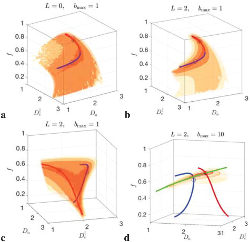
depending on the maximal invariant L used, Eq. (7). Contour surfaces are darker for lower values of F. Low-“energy” landscape of nonlinear RotInv problem (7) for system (6) is a 2-dimensional surface for l = 0 invariant (a), and two 1-dimensional trenches with l = 0, 2 invariants included (b, c). The trenches can either match to form a single 1-dimensional manifold (b), or be disjoint (c, d), depending on the ground truth values (see Supplementary Figs. S.1–S.2). Circles denote minima in both trenches, with the true minimum marked by *. Exact branches ξ = ± of system (11) (Sec. 2.5) are drawn in red and blue, reproducing the trenches up to 𝒪(b²). Including large b data further limits the landscape to the surface $f/\sqrt{D_a}$ arising solely from intra-neurite space (Jensen et al., 2016; Veraart et al., 2016b) (green section in d), helping, but not fully curing all degeneracies (see text and Figs. S.1–S.2).

Figure 3. Parametric maps for both branches (LEMONADE and nonlinear RotInv estimation), and prevalence maps.

Exemplary maps for subject 1, mid-brain axial slice. The branch maps (last column) are calculated using Eq. (13) based on the voxel-wise estimated parameters, with ξ = ± corresponding to red/blue. lemo±: outputs of LEMONADE ξ = ± branches, respectively (solution of Eqs. (11)), using only the shells within 0 ≤ b ≤ 2.5. Note that f₊ > f₋, as well as $D_{a+}>D_{e+}^{\Vert }$ and $D_{a-}<D_{e-}^{\Vert }$, practically consistent with Eq. (13). For ξ = + branch, the output $D_e^{\Vert }\gtrsim D_e^{\perp }$ is likely to be a result of the bias of moments estimation (a similar bias was observed in numerical simulations), since it is biophysically more plausible that $D_e^{\Vert }⊳D_e^{\perp }$. In a few voxels, the branch index ξ flips due to noise and partial volume effects affecting solution of Eqs. (11e)–(11f). RotInv±: Full nonlinear estimation outputs of gradient-descent minimization, Eq. (7), using all b shells, initialized via the corresponding lemo± maps. We observe the same qualitative features as in the LEMONADE maps, while numerically bringing $D_e^{\Vert }$ and $D_e^{\perp }$ closer. Importantly, the branch index ξ is fairly stable (cf. also histograms in Fig. 4) — for the vast majority of voxels, the nonlinear fitting of the full problem (7) does not change the branch index ξ = ± calculated based on the estimated parameters. lemo ξ: Selecting the LEMONADE branch ξ = ± voxel-wise, based on the proximity of the solutions for the redundant Eqs. (11e) and (11f), cf. Sec. 4.4 for details. RotInv ξ : Full RotInv output based on lemo ξ from previous row. Prevalence: Maps generated using the prevalence method (see text), current proxy for the ground truth. Note quantitative similarity of the parameter maps between RotInv ξ and prevalence. Extra-axonal diffusion tensors are practically always prolate, with $D_e^{\perp }$ values typically below 1, while D_a and $D_e^{\perp }$ around 2.

Figure 5. ROI values.

Mean ROI values for the 3 subjects, based on the prevalence method, in 10 standard WM ROIs (JHU atlas), as well as in all WM and GM voxels. The maximal water diffusivity value 3 μm²/ms for the body temparature is drawn as red lines for D_a and $D_e^{\Vert }$. Inter-ROI variability clearly exceeds inter-subject variability for f and p₂; the ROI differences in diffusivities are present albeit less pronounced. The ‘branch’ values are calculated based on ROI means according to Eq. (13), while the corresponding β values are calculated voxel-wise, and averaged over ROIs. The ξ = + branch would correspond to β falling in-between the two red lines, and ξ = − otherwise, cf. Eq. (13). Branch assignment based on the fairly noisy estimates of β is not robust and needs further validation.

Figure 4. Degeneracy in parameter estimation with human dMRI data as bimodality in parameter histograms.

Parameter histograms for WM, a, and for GM, b. Red/blue dashed histograms correspond to $\zeta =\pm \text{solutions}{\{f,D_a,D_e^{\Vert },D_e^{\perp },p_2\}}_{\pm }$ of LEMONADE system (11); filled histograms are obtained via RotInv fitting (7) up to b ≤ 10, initialized by the ξ = ± solutions of system (11). The last column shows the branch selection parameter β, Eq. (13), with the red/blue intervals corresponding to the ± branches. Nonlinear fitting (7) brings the D_a and $D_e^{\Vert }$ values closer to each other, and reduces $D_e^{\perp }$, as in the maps in Fig. 3. Green dashed and solid histograms correspond to the branch selection method of Sec. 4.4 (cf. Fig. 3, lemo ξ) and the respectively initialized full RotInv output (Fig. 3, RotInv ξ). Note the qualitative and quantitative agreement between the voxel-wise branch selection output of RotInv (green) and prevalence method (black) described in Sec. 4.4.

Figure 6. ODF dispersion, local kernel-based tractography, and parameter maps.

a, Fiber orientation dispersion angle θ_disp from p₂ (prevalence method) emphasizes major WM tracts. b, Empirical reference ODF ℘⁽⁰⁾ (left, see text and Appendix G), and the fiber ODF calculated using p_lm from Eq. (3) (right), for the b = 5 shell, with l ≤ l_max = 6. Note the strong ODF sharpening effect, due to the deconvolution with locally estimated kernels K_l(b, x). c, Coronal view of a structural MR image (MPRAGE) overlaid with a reconstruction of the corticospinal fiber tract colored according to the value of the respective parametric maps x and p₂ (via prevalence method, Fig. 3) at each point along the track. Fiber tracts have been reconstructed using improved probabilistic streamline tractography (Tournier et al., 2010) by integration over local fiber ODFs calculated using p_lm estimated from Eq. (3) using the voxel-wise estimated kernel K_l(b, x), for the b = 5 shell with maximal SH order l_max = 6.

Figure 7. Are the scalar model parametersf, D_a, $D_e^{\Vert }$ and $D_e^{\perp }$ independent?

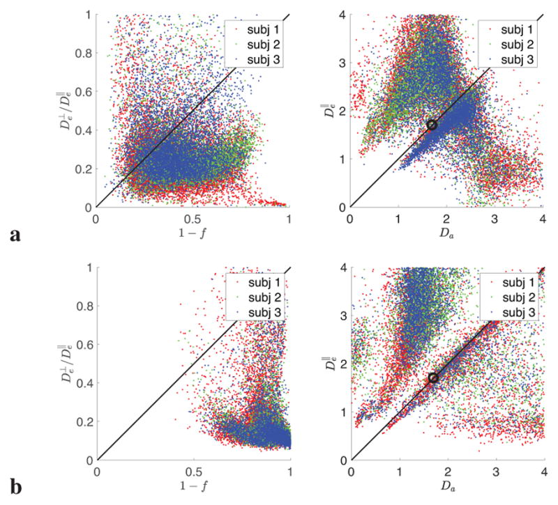
To see whether we can rely on relations between the scalar parameters in order to increase precision in their estimation, we investigate the validity of widely used constraints (Alexander et al., 2010; Zhang et al., 2012; Tariq et al., 2016; Kaden et al., 2016a) using parameter values estimated from the prevalence method. Generally, these constraints fail. Colors correspond to 3 subjects in WM(a) and GM (b). Interestingly, constraints fail more dramatically in GM.

2. Theory

2.1. Scalar-tensor factorization and rotational invariants

Signal (1) factorizes in the SH basis for any kernel 𝒦 (Healy et al., 1998; Tournier et al., 2004; Anderson, 2005; Jespersen et al., 2007; Jian and Vemuri, 2007; Dell’Acqua et al., 2007),

$$S_{lm}(b,x)=p_{lm}{K}_l(b,x).$$ (3)

Here S_lm and p_lm are the SH coefficients of the signal S and of the ODF

$$\mathcal{P}(\widehat{\mathbf{n}})\approx 1+\sum _{l=2,4,\dots }^{l_{max}}\sum _{m=-l}^l{p}_{lm}{Y}_{lm}(\widehat{\mathbf{n}}),$$ (4)

up to order l_max which practically depends on the dMRI sampling and signal-to-noise ratio (SNR), as it will be discussed below. The functions K_l(b, x) are projections of our model kernel (2) onto the Legendre polynomials (Eq. (A.2) in Appendix A) for a given set $x=\{f,D_a,D_e^{\Vert },D_e^{\perp }\}$ of scalar parameters.

To factor out the dependence on the choice of the physical basis in three-dimensional space (via m = −l ...l), recall that any rotation corresponds to an orthogonal transformation on the (2l + 1)-dimensional vectors S_lm and p_lm, belonging to the irreducible representation of the SO(3) group of rotations of weight l. Hence, the 2-norms ${\Vert S_l\Vert }^2={\sum }_{m=-l}^l{\mid S_{lm}\mid }^2$ and ${\Vert p_l\Vert }^2={\sum }_{m=-l}^l{\mid p_{lm}\mid }^2$ do not depend on the choice of the physical basis. Introducing basis-independent rotational invariants

$$S_l\equiv \Vert S_l\Vert /{\mathcal{N}}_l,p_l\equiv \Vert p_l\Vert /{\mathcal{N}}_l,{\mathcal{N}}_l=\sqrt{4\pi (2l+1)}$$ (5)

of the signal and ODF [cf. (Kazhdan et al., 2003) for using such approach for image matching in computer vision, (Mirzaalian et al., 2016) for dMRI data harmonization, and (Reisert et al., 2017) for the related machine-learning dMRI parameter estimation framework], the ODF SHs p_lm are factored out:

$$S_l(b,x)=p_l{K}_l(b,x),l=0,2,\dots .$$ (6)

Here, p₀ ≡ 1 (ODF normalization); the remaining ODF invariants, one for each l, characterize its anisotropy, with the normalization factor 𝒩_l chosen so that 0 ≤ p_l ≤ 1 (cf. Appendix B).

It now appears logical to first estimate the scalar parameters x, together with just a few basis-independent p_l, l = 2,..., from the greatly reduced system of equations (6), one for each l. A standard way to solve any such nonlinear system is to minimize the corresponding “energy” function

$$F^2(x,\{p_l\})\equiv \frac{1}{(1+\frac{L}{2})N_b}\sum _{l=0,2,\dots }^L\sum _{j=1}^{N_b}{w}_{lj}{[S_l(b_j,x)-p_l{K}_l(b_j,x)]}^2$$ (7)

with respect to x and a few p_l, l = 0, 2,..., L. We will refer to Eq. (7) as the rotationally invariant (RotInv) nonlinear objective function for minimization. Here b_j are the radii of N_b shells in q-space for a uniform spherical sampling; all units for diffusion coefficients and for 1/b are μm²/ms hereon. The weights $w_{lj}=1/{\sigma }_{lj}^2$ are chosen for the optimal precision, in terms of the effective noise variances ${\sigma }_{lj}^2~(2l+1)/N_j$ in each shell, after estimating 2l +1 independent parameters p_lm over the N_j diffusion directions in the shell b = b_j.

The estimated scalar parameters x will allow us to reconstruct the kernel components K_l(b, x), and to subsequently evaluate all ODF coefficients p_lm using Eq. (3), based on the linearly estimated S_lm from the measured signal — much like in a spherical deconvolution approach (Tournier et al., 2004, 2007), albeit with the voxel-wise, rather than globally estimated kernel (2), cf. (Anderson, 2005; Barmpoutis et al., 2009; Schultz and Groeschel, 2013).

While the above rotationally invariant framework looks conceptually simple and completely general [cf. (Anderson, 2005; Jespersen et al., 2007; Reisert et al., 2017)], the rest of this paper will be devoted to uncovering and resolving hidden degeneracies of parameter estimation problem (1) because of the kernel (2) specific to multi-compartmental diffusion in neuronal tissue. Understanding these degeneracies is essential for proper initialization and/or constraining any kind of solution for nonlinear system (6), e.g. via minimization of Eq. (7), or by machine learning methods (Reisert et al., 2017). This is especially relevant because it has been known all too well that direct nonlinear fitting of model (1)–(2) to realistic noisy data is unreliable. Hence, parameter estimation from clinical acquisitions has so far reverted to making severe restrictions on the ODF shape: either assuming a highly aligned bundle (Fieremans et al., 2010, 2011, white matter tract integrity (WMTI)), or a special Gaussian-like ODF shape characterized by one (Zhang et al., 2012, NODDI) or two (Tariq et al., 2016) parameters, in order to reduce the dimensionality of the problem by an order of magnitude.

Furthermore, the problem (7) has multiple degenerate minima, as we will investigate in detail below in Sec. 4, cf. Fig. 2. This echoes our previous recent study, where, even assuming the simplest, 1-parameter ODF shape (Zhang et al., 2012), unconstrained nonlinear fitting reveals multiple biophysically plausible minima in the (4+1) - dimensional parameter space, and flat directions along them (Jelescu et al., 2016a). Fixing all diffusion coefficients in Eq. (2) and ODF shape ℘(n̂) in Eq. (1), as done in NODDI (Zhang et al., 2012; Tariq et al., 2016), introduces a priori unknown bias (Jelescu et al., 2016a) for the remaining few parameters, and thereby leads to the loss of specificity — the main motivation for employing microstructural modeling. For example, diffusivity changes were recently found (Khan et al., 2016) in regions with no detectable neurite density changes; these details would otherwise have been lost or attributed to other parameters in an analysis using fixed diffusivities.

To understand analytically the information content of our acquisitions, in the rest of this Section we analyze the parameter estimation for the model (1)–(2) perturbatively in b. This approach is based on the Taylor expansion of the signal (1)

$$\frac{S_{\widehat{\mathbf{g}}}(b)}{S_0}=1-b{M}_{i_1{i}_2}^{(2)}{g}_{i_1}{g}_{i_2}+\frac{b^2}{2!}{M}_{i_1\dots i_4}^{(4)}{g}_{i_1}\dots g_{i_4}-\dots$$ (8)

in the fully symmetric moment tensors $M_{i_1\dots i_l}^{(l)}$. (Einstein’s convention of summation over repeated indices is assumed hereon.) The expansion in moments has a one-to-one correspondence with the cumulant expansion of ln S_ĝ (b) (Kiselev, 2010), and is also equivalent to Taylor-expanding the above nonlinear equations (3), (6), and (7), matching the moments of the signal and of the model at each order in b.

The perturbative approach, which we develop term-by-term in b, is useful in the three ways. First, it enables us to elucidate the role of the order l_max in Eq. (4), via the radial-angular connection in the q-space, Sec. 2.2, and to count the number N_p(l_max) of model parameters, which depends on the maximal even power l_max of the diffusion weighting q^l_max ~ b^l_max/2 to which an acquisition is sensitive, at a given signal-to-noise ratio (SNR), Sec. 2.4. Second, it helps us to develop intuition by analytically studying the problem’s degeneracies, Sec. 2.5, which will qualitatively persist in the subsequent full non-perturbative numerical treatment. Third, it will help initialize the full, non-perturbative numerical parameter estimation, Eq. (7) above.

2.2. Radial-angular connection in the q-space

Expanding the model (1)–(2) in the powers of b, one can readily see that moments $M_{i_1\dots i_l}^{(l)}$ are proportional to angular averages 〈n_i1 ... n_il 〉 over the ODF ℘(n̂). This follows from expanding the exponential terms containing ξ = n_ig_i in kernel (2), so that subsequent terms have the form b〈n_in_j〉g_ig_j, b²〈n_i1 ... n_i4 〉 g_i1 ... g_i4, etc (cf. Appendix C for explicit formulas up to l = 6).

It is crucial that the maximal even order l of the product 〈n_i1 ... n_il 〉 always appears with the corresponding power q^l ~ b^l/2 of the diffusion weighting. This observation underpins the perturbative radial-angular connection in the q-space: Practical sensitivity to the maximal order q^lmax automatically sets the sensitivity to the maximal order 〈n_i1 ... n_ilmax 〉 of the ODF average, and, therefore, to the maximal order l_max in its SH expansion (4). This key relation between the expansion (8) of the signal (1) and of the ODF (4) rests on the fact that linear combinations of symmetric tensors n_i1 ... n_il form the SH set Y_lm(n̂) (cf. Eq. (C.3) in Appendix C). Therefore, linear combinations of the ODF averages 〈n_i1 ... n_il 〉 correspond to the ODF SH coefficients p_lm.

The physical coupling between products q_i1 ... q_il in q-space imaging (Callaghan et al., 1988) and the ODF averages 〈n_i1 ... n_il 〉 emphasizes the preferred role the SH basis plays in dMRI. Essentially, the q-space measurement directly couples to the SH basis coefficients. Since we do not know the functional form of the ODF shape a priori, we cannot claim that we are able to determine ODF sharper than what is permitted by the practical sensitivity to the corresponding order q^l_max.

Hence, if our acquisition is only sensitive to, e.g. 𝒪(q⁴ ~ b²) (equivalent to diffusion kurtosis imaging, or DKI (Jensen et al., 2005)), parametrizing the ODF with p_lm with l > 4 would amount to ODF overfitting. Conversely, apparent sensitivity to p_lm up to order, e.g., l_max = 6, is equivalent to the presence of notable 𝒪(b³) contributions for a given b-shell (at a given SNR level). At finite b, the corresponding K_l(b) values numerically connect the radial and angular sensitivities in the q-space. We will turn to this point in Discussion, Sec. 5.1.

2.3. Parameter count: Signal via its moments, term-by-term

Let us count the number of parameters in expansion (8) as a function of the maximal order l_max. A term $M_{i_1\dots i_l}^{(l)}$ of rank l is a fully symmetric tensor, which can be represented in terms of symmetric trace-free (STF) tensors of rank l, l − 2, ..., 2, 0. Each set of STF-l tensors realizes a 2l + 1-dimensional irreducible representation of the SO(3) group of rotations, equivalent (Thorne, 1980) to the set of 2l+1 SH Y_lm (cf. Appendix C). Hence, the total number of independent components in the rankl moment (or cumulant) is $n_c(l)={\sum }_{l^{\prime }=0,2,\dots }^l(2l^{\prime }+1)=\frac{1}{2}(l+1)(l+2)$. Truncating the series (8) at l = l_max means that we determine all components of $M_{i_1\dots i_l}^{(l)}$ for l = 0,2,...,l_max, with the total number of independent, i.e. “informative”, components

$$N_c(l_{max})=\sum _{l=2,4,\dots }^{l_{max}}{n}_c(l)=\frac{1}{12}{l}_{max}^3+\frac{5}{8}{l}_{max}^2+\frac{17}{12}{l}_{max}$$ (9)

corresponding to N_c = 6, 21, 49, 94 ... for l_max = 2, 4, 6, 8 ... . (We did not include the unweighted S ₀ in our counting.) Eq. (9) returns familiar numbers of DTI, DKI, etc components, which can be practically estimated via polynomial regression of ln S_ĝ (b).

2.4. Parameter count: Model (1)–(2), term-by-term

So far, we counted the parameters of the representation (8) of the signal in terms of its moments. This representation is completely general — it only respects the time-reversal symmetry of the problem (only even orders l are included). We now count the number of parameters defining the biophysical model (1)–(2) with ODF (4) up to l_max. The N_s = 4 scalar parameters from kernel (2) in the absence of CSF (or N_s = 5 if the CSF compartment is added), are complemented by l_max(l_max + 3)/2 tensor parameters p_lm, obtained as ${\sum }_{l=2,4,\dots }^{l_{max}}(2l+1)\equiv n_c(l_{max})-1$ (since $p_{00}\equiv \sqrt{4\pi }$ is set by the ODF normalization), yielding

$$N_p(l_{max})=N_s+l_{max}(l_{max}+3)/2.$$ (10)

Hence, N_p = 9, 18, 31, 48, ... for l_max = 2, 4, 6, 8, ... already for the two-compartment kernel (2), without including S₀ and CSF fraction in the count.

Equation (10) reveals that the model complexity grows fast, as $l_{max}^2$ due to the ODF, if we are to account for the rich orientational content of the realistic fiber ODFs in the brain. For the achievable l_max ~ 4–8, the dMRI signal in principle “contains” a few dozen parameters, none of which are known a priori.

A superficial reason for poor fit quality is the high dimensionality (10) of the parameter space. However, comparing N_c(l_max) with the corresponding number of model parameters N_p(l_max), it naively looks like the series (8) is overdetermined, N_c ≥ N_p, already for l_max ≥ 4 — meaning that the acquisition looks sufficiently informative starting from the DKI level.

Unfortunately, this simplistic parameter count does not present the full picture, as the information content is not evenly distributed among all the N_c(l_max) components. It turns out that for l_max = 4 (DKI), there are not enough relations for scalar model parameters x, while too many for tensor parameters p_lm. All model parameters can be determined from the series (8) only starting from l_max ≥ 6, as we will now explain.

2.5. Perturbative approach to model (1)–(2): LEMONADE

In Appendix C, we derive the LEMONADE system of equations (C.6), relating the linear combinations of the signal’s moments to the model parameters. The rotationally invariant form of the LEMONADE system, one of the central results of this work, is as follows:

$$M^{(2),0}=f{D}_a+(1-f)(3D_e^{\perp }+{\mathrm{\Delta }}_e)$$ (11a)

$$\frac{M^{(2),2}}{p_2}=f{D}_a+(1-f){\mathrm{\Delta }}_e$$ (11b)

$$M^{(4),0}=f{D_a}^2+(1-f)\left[5{D_e^{\perp }}^2+\frac{10}{3}{D}_e^{\perp }{\mathrm{\Delta }}_e+{{\mathrm{\Delta }}_e}^2\right]$$ (11c)

$$\frac{M^{(4),2}}{p_2}=f{D_a}^2+(1-f)\left[\frac{7}{3}{D}_e^{\perp }{\mathrm{\Delta }}_e+{{\mathrm{\Delta }}_e}^2\right]$$ (11d)

$$M^{(6),0}=f{D_a}^3+(1-f)\left[7{D_e^{\perp }}^2(D_e^{\perp }+{\mathrm{\Delta }}_e)+\frac{21}{5}{D}_e^{\perp }{{\mathrm{\Delta }}_e}^2+{{\mathrm{\Delta }}_e}^3\right]$$ (11e)

$$\frac{M^{(6),2}}{p_2}=f{D_a}^3+(1-f)\left[\frac{21}{5}{D_e^{\perp }}^2{\mathrm{\Delta }}_e+\frac{18}{5}{D}_e^{\perp }{{\mathrm{\Delta }}_e}^2+{{\mathrm{\Delta }}_e}^3\right].$$ (11f)

Here ${\mathrm{\Delta }}_e\equiv D_e^{\Vert }-D_e^{\perp }$. The system (11) involves rotationally invariant components M^(L),l [defined in Eq. (C.7)] of the tensors $M_{i_1\dots i_l}^{(l)}$, up to minimal orders L ≤ 6 and l ≤ 2, enough to find all 4 scalar kernel parameters x, and ODF anisotropy invariant p₂.

The first four LEMONADE equations, corresponding to l_max = 4, contain 5 unknowns. (Introducing an extra equation M^(4),4 ∝ p₄ does not help, as it introduces yet an extra unknown ODF invariant p₄.) This is why the l_max = 4 acquisition, equivalent to relying on the signal’s curvature, or kurtosis, is fundamentally insufficient. This is an important fundamental limitation for the parameter estimation in the Standard Model.

The full system’s 6 equations are in principle enough to determine 5 model parameters; even with added CSF compartment with its fraction and an isotropic D_CSF = 3 μm²/ms, one could in principle still determine the 6 parameters from the appropriately modified system (11). At the l_max = 6 level, one could introduce even more equations: M^(6),4 ∝ p₄, or M^(6),6 ∝ p₆, at the expense of extra unknown ODF invariants p₄ and p₆. Practically, they would rely on the components M^(L),l with high l, which are less accurately estimated. Tying p_l with different l to each other could be a way to increase precision, but at the expense of constraining the ODF shape to a particular functional form. Therefore, the LEMONADE system (11) is minimally complex yet still fully unconstrained. LEMONADE is solved exactly in Appendix D, and its output is subsequently used to initialize the subsequent nonlinear minimization, Eq. (7) in Sec. 2.1 above.

Crucially, LEMONADE, and hence the original nonlinear problem (7), has multiple biophysically plausible solutions. The choice of the physical solution, to initialize problem (7), is nontrivial, Sec. 4.1; in Sec. 4.4 below we will rationalize our recipe for making such selection voxel-wise. In the Methods, Sec. 3.4 and Fig. 3, we summarize all RotInv computational steps.

3. Methods

3.1. In vivo dMRI

Three healthy volunteers underwent imaging on a Siemens Prisma 3T whole-body MRI scanner. The study was approved by the local Institutional Review Board, and informed consent was obtained and documented from all participants. The MRI scanner was equipped with a 80 mT/m gradient system and a 64-channel receiver head coil. The body coil was used for transmission. A monopolar diffusion-weighted EPI sequence was used to acquire the dMRI data. Diffusion weighting was applied along 64 isotropically distributed gradient directions for each of the 21 b-values equidistantly distributed in the range [0 : 0.5 : 10] ms/μm². Following imaging parameters were kept constant throughout the data acquisition sequence: TR/TE : 4000/105 ms, matrix: 80 × 80, NEX: 1, in-plane resolution: 3 × 3 mm², slice thickness: 3 mm, slices: 38, parallel imaging: GRAPPA with acceleration factor 2, reconstructed using the adaptive combine algorithm to ensure Rician data distribution, multiband acceleration with factor 2, and no partial Fourier. Total scan time was just below 2 hours per person.

3.2. Image processing

MP-PCA noise estimation and denoising method (Veraart et al., 2016a,c) allowed us to preserve only the significant principal components and to strongly reduce the noise in the data and to estimate spatially varying noise map. The positive signal bias, inherent to low-SNR magnitude MR data, was removed by using the method of moments (Koay and Basser, 2006), where the denoised signal was used as a proxy for the Rician expectation value. Denoised and Rice-floor-corrected images were subsequently corrected for Gibbs ringing (Kellner et al., 2016), geometric eddy current distortions and subject motion (Andersson and Sotiropoulos, 2016).

3.3. Estimating moments from dMRI signal

Expansions in moments and in cumulants are mathematically equivalent; the combinatorial relation between moments and cumulants (“linked cluster expansion”) was established in statistical physics (Mayer and Montroll, 1941), and is reviewed in (Kiselev, 2010). While expanding in moments (8) is the most optimal for the analytical treatment (contributions from different tissue compartments add up), we observe that estimation from the dMRI signal is more accurate from the cumulant series. Hence, for accuracy, we first estimate the cumulant tensors C^(l)

$$ln\frac{S_{\widehat{\mathbf{g}}}(b)}{S_0}=-b{C}_{i_1{i}_2}^{(2)}{g}_{i_1}{g}_{i_2}+b^2{C}_{i_1\dots i_4}^{(4)}{g}_{i_1}\dots g_{i_4}-\dots$$ (12)

and the unweighted S₀, via b-matrix pseudoinversion applied to ln S_ĝ (b), with voxel-specific weights (Veraart et al., 2013) up to l_max = 6. We then convert $C_{i_1\dots i_l}^{(l)}$ to the moments $M_{i_1\dots i_l}^{(l)}$ as derived in Appendix E. For unbiased estimation, we use only shells within 0 ≤ b ≤ 2.5, where the cumulant series is expected to converge.

3.4. Implementation and computation time

Processing steps (Fig. 3) were implemented in Matlab (Math-Works, Natick, MA, USA), according to Eqs. (12), (C.5), (C.7), and (D.1)–(D.7) using standard library functions, and the Levenberg-Marquardt algorithm for subsequent nonlinear minimization of Eq. (7) initialized by LEMONADE output x and p₂. For the whole brain (34383 voxels within the WM+GM mask for subject 1, at our relatively coarse resolution) on a desktop iMac (4 cores), it took under 2 min for estimating the cumulants using the b-matrix pseudoinversion with the voxel-specific weights (Veraart et al., 2013), together with recalculating the moments (C.5) from the cumulants, Appendix E (only the range b ≤ 2.5 was used for unbiased estimation); 1.5 min for LEMONADE calculation (both branches); and ~ 5 min for nonlinear fitting, Eq. (7), including all shells, using the corresponding LEMONADE solution (Sec. 4.4) as fit initialization. Nonlinear fitting achieves speedup because of the initial values being already quite close to the minima of F; we also precomputed corresponding integrals (A.2) and their first derivatives in a broad range.

4. Results

4.1. Topology of parameter landscape

The contour plots of values of RotInv energy function F, Eq. (7), shown in Fig. 2 (cf. also Supplementary Figs. S.1–S.2 for more examples), illustrate that the minimization landscape is generally quite flat in at least 1 dimension, and there exist multiple minima. We emphasize from the outset that these degeneracies are intrinsic to the problem (1)–(2), and are not introduced by the above RotInv framework or the particular way (7) of solving the system (6). Rather, this framework allows us to uncover their general origin – namely, the multi-compartmental character of the kernel (2).

We now focus on the topology of the low-energy landscape of F in order to understand degeneracies in parameter estimation, which is crucial for initializing the search for parameters x within the biophysically correct domain, and for speeding up the solution of system (6). As mentioned in Theory Section above, our analytical method to study this topology, is to approximate the signal (1) by its low-b expansion (8), whose consecutive terms are equivalent to diffusion tensor imaging (DTI, ~ b), diffusion kurtosis imaging (DKI, ~ b²), etc. Empirically, it is known that DKI (Jensen et al., 2005) approximates clinical dMRI signal (b_max ~ 1 – 2) quite well, further justifying studying the series (8) up to 𝒪(b²), and perhaps, up to 𝒪(b³).

For low enough b (typically used in the clinic), nonlinear fitting (7) practically corresponds to matching first few moments of the signal (8) to those of the model (1). In Sec. 2.5 above we exactly derived this matching, the LEMONADE system (11), for up to 𝒪(b³). We can now calculate the dimensionality of the low-energy “attractor” manifolds in Fig. 2 by simple counting of equations.

Taking the l = 0 invariant alone, S ₀ = K₀, is exactly equivalent to isotropic (or “powder”) signal averaging (Jespersen et al., 2013; Lasic et al., 2014), a result subsequently used in the “spherical mean technique” (SMT) (Kaden et al., 2016b,a). Expanding the relation S₀ = K₀ up to 𝒪(b²) yields a 2-dimensional surface, in accord with the two equations (11a) (~ b) and (11c) (~ b²) for the 4 scalar parameters x, cf. Fig. 2a (note that isotropic averaging discards nontrivial p_l with l > 0). This rationalizes the empirical need for the 4 – 2 = 2 constraints introduced in the SMT; their validity will be discussed in Sec. 5.2 below. While, theoretically, the l = 0 technique allows one to factor out the ODF, we can see that practically determining all 4 scalar parameters x from the single invariant K₀ requires the sensitivity to the signal’s moments up to M⁽⁸⁾ (namely, to their full traces), i.e. up to b⁴ in expansion (8), which is extremely hard to achieve. Intuitively, it is quite obvious that discarding the orientational content of the signal makes parameter estimation less informative.

According to the analysis in Sec. 2.5 above, staying at the same level 𝒪(b²), and including the K₂(b) invariant, L = 2, adds one extra parameter p₂ describing the sensitivity to the lowest-order ODF anisotropy, and two extra equations, (11b) and (11d), turning the surface into the two narrow 1-dimensional trenches in parameter space, Fig. 2b,c (the first 4 equations of the system (11) for 5 parameters: x and p₂). Having a perfectly flat trench is obvious from the counting of equations; getting what looks like two trenches is nontrivial.

The trenches f_ξ(p₂) (Eq. (D.7) in Appendix D), labeled by branch index ξ = ±, Eq. (D.8), represent the exactly derived “flat” one-dimensional continuous manifold that involves rotationally invariant combinations of signal’s moment tensors M⁽²⁾ and M⁽⁴⁾. The parameterization of this manifold, derived as the two branches of quadratic equation (D.4), makes it appear within the physically meaningful domain of parameters as either one trench (the ξ = ± parts merge), Fig. 2a,b, or as two disjoint trenches, Fig. 2c, depending on the ground truth values. Physically, the dual branches come from having two tissue compartments, cf. the “toy model” of Appendix F. There, we emphasize that both sets of values (obtained after imposing an extra constraint p₂ = p₄ = 1 of a single-fiber case) can look perfectly plausible, and the “wrong” set corresponds to swapping intra- and extra-neurite parameters — which carries the danger of misrepresenting parameter changes in pathology. Including the K₄(b) invariant adds one extra parameter p₄ and only one equation for M^(4),4 (since K_l(b)|_b→0 ~ b^l/2); hence, further invariants K_l>2 do not provide extra equations relative to the number of unknowns up to b².

As a result, if an acquisition is only sensitive to 𝒪(b²), due to e.g. b-range or SNR limitations (as it is often the case in the clinic), the parameter estimation problem will be in general “doubly degenerate”, as we empirically observed recently for a particular ODF shape (Jelescu et al., 2016a): with respect to selecting the trench (discrete degeneracy), and due to the perfect flatness (zero curvature) along either trench (continuous degeneracy). Our exact solution of system (11) establishes that these two kinds of degeneracy are general “hidden” features of problem (1)–(2), due to every point in each branch exactly matching the b and b² terms in the Taylor expansion (8).

Furthermore, as already mentioned in Sec. 2.5, simplistic counting of parameters, without separating them into the scalar and ODF parts, can be misleading: the N_c(4) = 21 DKI parameters are not enough to determine the corresponding N_p(4) = 18 model parameters, Eq. (10), since the excess parameters over-determine the ODF, whereas the kernel (2) remains under-determined. (This issue becomes even more severe if the kernel has more than 2 compartments, e.g. by adding the CSF pool.) This means that, unfortunately, a popular DKI acquisition is not enough to resolve two-compartment model parameters due to a perfect 1-dimensional degeneracy within a chosen trench, unless, e.g., p₂ is fixed by the ODF shape: p₂ → 1, the aligned fibers assumption (Fieremans et al., 2010, 2011) (which still then requires making a discrete branch choice).

We also note that including the l > 0 invariants in system (6) is only possible for anisotropic ODFs, with p_l > 0. Physically, it is expected since the less symmetric the system, the more inequivalent ways it enables for probing its properties; this intuition has had far-reaching consequences in quantum theory of excitations of non-spherical nuclei (Bohr and Mottelson, 1998). For our classical physics purposes, it means that it is overall harder to determine parameters of gray rather than white matter. Fortunately, in the brain, ODF is at least somewhat anisotropic; the anisotropy parameter p₂ is generally nonzero even in the gray matter, as we can see a posteriori, cf. Figs. 3–5.

4.2. Bimodality of parameter estimation in human dMRI

In Figures 3 and 4 we demonstrate the double degeneracy of parameter estimation problem (1)–(2), anticipated from topology of Fig. 2, using a dedicated human dMRI acquisition (cf. Methods). We first solve the LEMONADE system (11) (using subset with b ≤ 2.5), map all parameters (cf. Fig. 3 lemo ±), and plot histograms for its both branches ${\{f,D_a,D_e^{\Vert },D_e^{\perp },p_2\}}_{\zeta =\pm }$ (red and blue dotted lines in Fig. 4) in white matter (WM, ~ 11,000 voxels), and in gray matter (GM, ~ 13,000 voxels), selected using probability masks. (WM mask was further thresholded by FA > 0.4 to exclude partial volume effects.)

We then use pairs of LEMONADE solutions with ξ = ± in each voxel to initialize the full gradient-descent nonlinear Rot-Inv minimization (7), for which all the data with b ≤ 10 is used (cf. Fig. 3 RotInv ±). This leads to the corresponding shaded histograms in Fig. 4. We can see that the output of full optimization (7) is qualitatively similar to that based on the Taylor expansion (8), with bimodal parameter histograms corresponding to the fundamental degeneracy of the parameter landscape corresponding to the two distinct branches of solutions.

Our analysis shows that the two branches are qualitatively distinct in the following ways: f₊ > f₋; also, usually, $D_a>D_e^{\Vert }$ for ξ = + and $D_a<D_e^{\Vert }$ for ξ = − (cf. Eq. (13) below). Generally, neither solution can be discarded based on parameter values alone, as they often fall within plausible biophysical bounds 0 < D ≲ 3 and 0 < f < 1. (We show up to D = 4 to illustrate the role of noise in broadening the histograms.) Figure S.4 in Supplementary Section S.3 shows that improvement in accuracy gained by nonlinear minimization (7) relative to LEMONADE occurs because small errors in estimated moments in the finite range of b translate into greater errors in the LEMONADE solutions, mostly due to errors in estimating the moment tensor M⁽⁶⁾.

4.3. Branch index ξ in terms of ground truth parameters

Our analysis in Fig. 3 (cf. branch column) and in Fig. 4 highlights the stability of the branch index ξ: The exact bimodality, following from the topology of minimization landscape at low b, still affects parameter estimation even at very high b, since the 𝒪(b³) terms and beyond generally result in a local minimum in either trench. Hence, branch assignment is akin to a discrete topological index, characterizing which part of the parameter space a given imaging voxel belongs to, based on its ground truth values.

In Appendix D, Eq. (D.8), we derive that the choice of the ξ = + branch corresponds to the ratio β between ground truth compartment diffusivities falling within the interval

$$4-\sqrt{\frac{40}{3}}<\beta <4+\sqrt{\frac{40}{3}},\beta =\frac{D_a-D_e^{\Vert }}{D_e^{\perp }},$$ (13)

and the ξ = − branch should be chosen otherwise.

Branch choice is nontrivial because we a priori do not know the ground truth values D_a, $D_e^{\Vert }$ and $D_e^{\perp }$ entering Eq. (13); besides, these values may generally vary across the brain, and be altered in pathology. Noise may affect estimated diffusivities enough to switch the estimated branch ratio β (Figs. 3–5 and S.4), which is particularly noisy due to the division by a small $D_e^{\perp }$ and its imprecise estimator.

4.4. Branch selection

Sensitivity to 𝒪(b³) terms and beyond, ideally, will determine which branch ξ = ± is the correct one, as well as the true minimum (solution) along this branch. Practically, however, branch selection from realistic noisy data turns out to be quite challenging. Relying on very large b data is also tricky: the scaling (Veraart et al., 2016b; McKinnon et al., 2016) $S~f/\sqrt{b{D}_a}$ for bD_a ≫ 1 is similar for both branches, since f₊ > f₋ and D_a+ > D_a−, compensating each other’s effect. (Note, however, the 1/b-scaling of the ODF variance suggested in (Veraart et al., 2016b) as a method to uncouple f and D_a; the precision of this uncoupling has so far been generally not enough to make a decisive branch choice for single fiber populations in WM.)

For now, to get the best available proxy for the ground truth, and to select the branch, we use our wide-b-range dedicated dMRI acquisition and calculate the scalar parameters independently of the branch location, solely based on the prevalence. In order to not bias our outcome on the branch choice, for each voxel, we initialize the problem (7) using 100 random starting points within the biophysically plausible parameter range (such as 0 < f, p₂ < 1, and 0 < D < 3 for all diffusivities), observe that the fit outcomes typically cluster around a few points in the parameter space, and select the mean of the largest cluster (after excluding the outcomes outside the plausible bounds). An increasing b-range broadens the basin of attraction of the true minimum in a model calculation (Jelescu et al., 2016a). Supplementary Fig. S.4 justifies this method using simulations for a range of ground truth values with added noise. Certainly, this method may still fail in some voxels, but the overall maps (Fig. 3 bottom row, and Fig. 6c) look sufficiently smooth and biophysically plausible. While we do not have an independent validation method for the prevalence parameters, we performed the prevalence calculation for all three subjects and observed that the prevalence maps and histograms are similar, as are their ROI values (Fig. 5).

Histograms of branch ratio (13) in Fig. 4, as well as branch maps in Fig. 3, unfortunately yield no clear branch selection depending on the ROI. It looks like the left inequality, $4-\sqrt{40/3}<\beta$, is practically most often choosing the branch, but this choice is inconclusive, cf. bottom two rows in Fig. 5 —presumably, due to the ground truth values varying across the brain, and because of the effects of the noise in estimating the three diffusivities. (Since typical $D_e^{\perp }\lesssim 0.5$, the left inequality may be practically often identified with $\zeta =sgn(D_a-D_e^{\Vert })$; however, the exact branch selection involves all three diffusivities.) There is a cluster of voxels with $D_a\approx D_e^{\Vert }$ such that $\beta \approx 4-\sqrt{40/3}\approx 0.35$ (cf. also Fig. 7); for those, branches merge since the discriminant 𝒟 → 0, Eq. (D.6), and both estimated parameter sets coincide.

Prevalence calculations take long time. Practically, since we cannot so far see any obvious “global” branch selection method, we tested choosing the branch voxel-wise, based on having the two redundant LEMONADE equations (11e) and (11f) for M^(6),0 and M^(6),2. As described at the end of Appendix D, their independent solutions for p₂ (after excluding all scalar parameters using the first 4 LEMONADE equations), which we label ${p_2}_{\zeta }^{(6),0}$ and ${p_2}_{\zeta }^{(6),2}$, produce the corresponding sets $x_{\zeta }^{(6),0}$ and $x_{\zeta }^{(6),2}$ of scalar parameters, for both branches. Only the correct solution would yield the same set of parameters $x_{\zeta }\equiv x_{\zeta }^{(6),0}=x_{\zeta }^{(6),2}$ when using either of these two equations. Noise inevitably causes the discrepancy between the solutions $x_{\zeta }^{(6),0}$ and $x_{\zeta }^{(6),2}$ even for the correct branch ξ; however, for sufficiently small noise, these solutions in the correct branch will be closer to each other than those for the wrong branch. This branch choice, cf. Appendix D, is reasonable for SNR = 100 (and not very conclusive for the SNR = 33), Supplementary Fig. S.4. Its output, taken as the mean between the sets $x_{\zeta }^{(6),0}$ and $x_{\zeta }^{(6),2}$ for the chosen ξ is shown in Fig. 3 (lemo ξ row), and Fig. 4 (dashed green lines). We then use it to initialize the full nonlinear RotInv problem (7), which leads to the output marked by RotInv ξ in Fig. 3 and by solid green lines in the histograms of Fig. 4. We can see that this output generally matches quite well the results of the prevalence method. Furthermore, we observe strong similarity in the ROI-averaged values between both methods, Fig. 5 and Supplementary Fig. S.3.

4.5. ODF and fiber tracking using locally estimated kernels

Figure 6b demonstrates that fiber ODFs (right panel), calculated using factorization relation (3), are notably sharper than the “reference” signal ODFs (left panel). Here, we calculated the SH coefficients of the reference signal ODF ℘⁽⁰⁾ via $p_{lm}^{(0)}={(-)}^{l/2}{S}_{lm}$, cf. Appendix G. The logic was to maximally preserve the “raw” diffusion-weighted signal, and to only rotate its l = 2,6,10,... harmonics, so that the directionality of the resulting ℘⁽⁰⁾ mimics that of the genuine fiber ODF, while the blurring due to the diffusion is preserved. We notice that the projections (A.2) of the kernel onto the Legendre polynomials have the alternating sign (−)^l/2, which physically turns a prolate fiber ODF into an oblate signal. In Appendix G we show that such a procedure corresponds to a (de)convolution with a singular kernel, concentrated along the equator ξ = n̂ · ĝ = 0 of the unit sphere n̂ = 1 (relative to the diffusion direction ĝ), akin to the Funk-Radon transform (Tuch, 2004; Descoteaux et al., 2009; Jensen et al., 2016) — albeit taking a fractional derivative ${{\partial }_{\xi }^{1/2}\mid }_{\xi =0}$ in the direction transverse to the equator, instead of merely averaging over the equatorial points via δ(ξ), as in the FRT. Such a “blur-preserving” procedure can serve as a natural reference for the model-based ODF deconvolution methods. Note that the coefficients |K_l(b)| generally decrease with l. Therefore, dividing by the kernel K_l(b) gives larger weight (relative to (−)^l/2) to the higher-order spherical harmonics, sharpening the fiber ODF relative to ℘⁽⁰⁾, Fig. 6b. Small spurious ODF peaks are intrinsic to unconstrained SH deconvolution due to low order truncation and thermal noise (Tournier et al., 2004), and might be further mitigated by adopting the constrained approaches (Tournier et al., 2007). Here, we show all parameters estimated without any constraints.

Fiber ODFs, rather than empirical signal ODFs, should be in principle a better starting point for any fiber tracking algorithm, as physics of diffusion is factored out. Figure 6c shows an example of the probabilistic tractography outcome, using iFOD2 algorithm with default settings (Tournier et al., 2010) as part of the MRtrix3.0 open source package by Tournier et al. (2012, www.mrtrix.org), relying on ODFs (4) using locally estimated kernels (2) via Eq. (3), with the scalar parameters and p₂ drawn on the streamlines. Furthermore, voxel-wise estimated f,D_a, $D_e^{\Vert },D_e^{\perp }$ and p_lm can serve as a starting point for mesoscopic global fiber tracking (Reisert et al., 2014) that can provide further regularization of problem (1)–(2) by correlating over adjacent voxels.

5. Discussion

The rotational invariant framework for the overarching model (1) generalizes previous methods which constrained parameter values or ODF shape, reveals a nontrivial topology of the fitting landscape, and explains its degeneracies, and associated issues with accuracy and precision in modern quantitative approaches to dMRI-based neuroimaging.

5.1. Parameter values

We observe that scalar parameter values in Fig. 3 (especially RotInv ξ and prevalence) exhibit WM/GM contrast, with the T₂-weighted axonal water fraction f highest in major tracts, approaching 0.7 – 0.8. The neurite fraction drops significantly in GM, down to about 0.2, in agreement with the recent study based on isotropic diffusion weighting (Lampinen et al., 2017). There could be a number of explanations to this observation. First, the T₂ values in extra- and intra-neurite spaces are generally different, which re-weighs the compartment fractions. In fact, in our recent RotInv-based work (Veraart et al., 2017), where we varied echo time for probing compartment T₂ values, we generally found $T_2^a>T_2^e$ for WM, effectively increasing the T₂-weighted fraction f in WM; this balance may be different in GM. Second, water within cell bodies in GM may effectively add to extra-neurite fraction (Chklovskii et al., 2002). Furthermore, such low fraction could be rationalized if some of neurites (e.g. dendrites or glia) happen to be in the intermediate or even fast water exchange regime as recently argued by (Yang et al., 2017); in this case, the low f ~ 0.2 could be dominated by myelinated axons whose fraction is lower in GM. In that case, model (1) for GM should be augmented by incorporating exchange and possibly time-dependence of effective diffusion metrics (Novikov et al., 2014; Fieremans et al., 2016).

Scalar parameters x do not abruptly differ between corpus callosum and the crossing regions such as centrum semiovale, cf. Fig. 6c, emphasizing that our approach is able to separate the spatially varying orientational dispersion ℘(n̂) from the kernel 𝒦. Conversely, p₂ drops significantly in WM crossing regions, Fig. 6c (panel p₂), as well as in GM (Fig. 3 and Fig. 6a). Typical fiber orientation dispersion angle θ_disp, calculated as ${\theta }_{\text{disp}}\equiv {cos}^{-1}\sqrt{\langle {cos}^2(\theta )\rangle }$, cf. Eq. (B.2) in Appendix B, delineates major WM tracts in Fig. 6a; the values θ_disp ≈ 20° in genu and splenium agree remarkably well with the range 14° – 22° observed recently from NAA diffusion and from histology in human corpus callosum (Ronen et al., 2014). Even stronger orientational dispersion occurs in other WM regions, stressing the need to account for it (Zhang et al., 2012; Tariq et al., 2016; Ferizi et al., 2015).

Relation (3) describes how fast the signal’s harmonics S_lm decrease as function of l. As an estimate, for a HARDI shell of b = 3, assuming $D_a\approx D_e^{\Vert }\approx 2$ and neglecting $D_e^{\perp }$, we numerically find (−)^l/2K_l ≈ {0.36, 0.14, 0.055, 0.019, 0.0055, 0.0014} for l = 0,2,...,10. This calculation gives an estimate of the highest SH order l to be observed in the signal S _lm, as function of SNR, assuming that p_lm are not small, and suggests l_max = 6 – 8 as a practical upper bound at typical in vivo SNR values, in agreement with numerical estimates (White and Dale, 2009) and an observation in voxels with single fiber populations (Tournier et al., 2013). Conversely, the same estimate tells that at reasonable SNR, involving the S₄(b) signal invariant to estimate scalar parameters may help only marginally (we did not see practical difference with our MRI data), while higher-order S_l(b) will likely drown in the noise. The decrease of K_l(b) with l and b embodies a non-perturbative analog of the perturbative radial-angular connection (Sec. 2.2).

5.2. Parameter (in)dependence and possible constraints

Overall, we find that all three diffusivities generally vary across brain. We also observe that D_a is estimated more precisely than $D_e^{\Vert }$ and $D_e^{\perp }$ (cf. Fig. S.4 in Supplementary Sec. S.3). This can be expected due to the extra-neurite space being suppressed by the factor $e^{-b{D}_e^{\perp }}$ relative to the intra-axonal one, cf. Eq. (2). Scatter plots in Fig. 7 confirm that $D_e^{\Vert }$ and $D_e^{\perp }$ should be generally estimated independently, since neither of the widely employed constraints of NODDI and SMT, $D_e^{\Vert }=D_e^{\perp }/(1-f),D_a=D_e^{\Vert }$ (Alexander et al., 2010; Zhang et al., 2012; Tariq et al., 2016; Kaden et al., 2016a) and $D_a=D_e^{\Vert }=1.7$ (Alexander et al., 2010; Zhang et al., 2012; Tariq et al., 2016) seem to be universally valid. Given the “shallow” fit landscape, employing unjustified constraints generally results in notable and unpredictable bias in the remaining parameters, which is likely to translate is unknown biases in parameter trends when applied to pathologies.

We can see that the tortuosity constraint $D_e^{\Vert }=D_e^{\perp }/(1-f)$ (left panels in Fig. 7) is especially questionable: the tortuosity $D_e^{\Vert }/D_e^{\perp }~5$ seems to be very high, as compared to the mean-field estimate (Szafer et al., 1995) used previously. The fact that the mean-field estimate fails, by ~ 100%, at the biologically relevant fiber packing densities has been previously shown both analytically and numerically (Novikov and Fieremans, 2012).

Whether $D_a=D_e^{\Vert }$ can be adopted as a constraint at least in some regions remains inconclusive. To test this assumption, we solved the LEMONADE system (11) exactly under the additional assumption $D_a=D_e^{\Vert }$, based on the first 4 equations, equivalent to 1 + d₂(p₂) = d_a(p₂), cf. Eqs. (D.2) in Appendix D; the branch selection for the corresponding quadratic equation

$$\left[9M^{(4),0}-5{(M^{(2),0})}^2\right]p_2^2+2\left[9M^{(4),2}-7M^{(2),0}{M}^{(2),2}\right]p_2=8{(M^{(2),2})}^2$$

is definitive in this case (always the + branch of the corresponding discriminant, since otherwise p₂ < 0), and all parameters x are given via simple explicit expressions (D.2) based on the found p₂. However, due to bias in the moments, as well as likely the inapplicability of the global constraint $D_a=D_e^{\Vert }$, the parameter values remain biased so that, for instance, often times f > 1. This solution also proved notably less optimal for initializing the full RotInv estimation (7) (unphysical values in many voxels, and overall lack of agreement with the prevalence outcomes). These observations speak against imposing such a global constraint on the diffusivities.

On the other hand, there is recent evidence that $D_a\approx D_e^{\Vert }$ in rat spinal cord (Skinner et al., 2017). Recent time-dependent diffusion study (Jespersen et al., 2017) in fixed porcine spinal cord favors the ζ = + branch. However, we note that spinal cord morphology, and effects of tissue fixation, can make these estimate sufficiently different from those in in vivo human brain. Overall, it remains an open question whether and by how much D_a and $D_e^{\Vert }$ differ, and by how much each of them changes in different pathologies.

At this time, we are not aware of relations between parameters able to constrain the problem without introducing bias. Precision improvement can come from “orthogonal” measurements (Dhital et al., 2015; Szczepankiewicz et al., 2015, 2016; Lampinen et al., 2017; Skinner et al., 2017; Dhital et al., 2017a,b) cutting through the trenches (as discussed below), as well as from searching for solutions within the physical parameter ranges for x (e.g. by creating libraries of K_l(b, x)), based on better understanding of the ground truth. This should be a subject of future work. 5.3. Branch selection and “orthogonal” measurements

Overall, our current branch choice method does not seem optimal, and we suggest that branch selection remains an essential problem for quantifying neuronal microstructure, to be ultimately validated using very strong diffusion gradients (e.g. employing unique Connectom scanners with gradients up to 300 mT/m), as well as adding “orthogonal” acquisitions such as extra-neurite water suppression by strong gradients (Skinner et al., 2017) and isotropic diffusion weighting (Dhital et al., 2015; Szczepankiewicz et al., 2015, 2016; de Almeida Martins and Topgaard, 2016; Lampinen et al., 2017). In particular, isotropic weighting (spherical tensor encoding), yielding

$$S(b)/S_0=f{e}^{-b{D}_a}+(1-f)e^{-b(D_e^{\Vert }+2D_e^{\perp })},$$ (14)

seems to produce relations $D_a\approx D_e^{\Vert }+2D_e^{\perp }$ due to an empirically small iso-weighted kurtosis of signal (14) (Dhital et al., 2015; Lampinen et al., 2017; Dhital et al., 2017a). While this can be interpreted as favoring the ζ = + branch, this relation cannot be used as a global constraint: Szczepankiewicz et al. (2015) show it failing in thalamus, apparently consistent with the ζ = – selection in GM (note however that thalamus is a GM/WM mixture). It is also interesting to further investigate the branch-merging case of $D_a\approx D_e^{\Vert }$ (Skinner et al., 2017).

We also note that branch selection (13) for the unconstrained problem (1)–(2) is qualitatively similar but quantitatively different from that in the WMTI highly-aligned tracts case (Fieremans et al., 2010, 2011), cf. the toy model of Appendix F. In Fig. 3 we see that the lemo– branch qualitatively corresponds to the standard WMTI choice $D_a<D_e^{\Vert }$, also preferring larger p₂ (strongly aligned fibers). While qualitatively, the “wrong branch” in both the full model (1)–(2) and WMTI (Fieremans et al., 2011) corresponds, roughly, to swapping of intra- and extra-neurite parameters, there is no exact correspondence; for instance, f and $D_e^{\perp }$ are also different between the branches. The difference between WMTI and the full model comes from the fact that in the toy model (WMTI prototype), the perfectly-aligned fiber constraint p₂ = p₄ = 1 has been implemented, together with effectively mixing the LEMONADE equations with moments M^(4),2m and M^(4),4m. Therefore, the branch choice based on $sgn(D_e^{\Vert }-D_a)$ is sufficiently different from that of Eq. (13).

5.4. Limitations and generalizations

Overall, our experience shows that it is quite difficult to estimate scalar parameters, even with a highly oversampled acquisition. The scalar-tensor factorization works in such a way, that while ODF parameters p_lm “lie on a surface”, scalar parameters are quite hidden, so that directional dMRI acquisition is not very sensitive to their values. Therefore, our unconstrained fit, Eq. (7), yields maps which for some parameters are quite noisy (Fig. 3), with unphysical values masked. Noise in voxelwise maps is not a bug but a feature: it arises from the degeneracies (“trenches”) in the landscape, Fig. 2, inherent to the general model (1)–(2). Similar issue has been empirically noted in the related machine-learning method (Reisert et al., 2017), where model degeneracies manifest themselves in priors strongly affecting the estimation outcome. Here, our goal has been to uncover and to understand the uncertainties in the unconstrained maps achieved with a very extensive directional human dMRI acquisition. Effect of noise is somewhat alleviated when looking through semi-transparent-drawn tracts (Fig. 6c), where the anatomical trends in all parameters become particularly obvious.

Our main limiting assumption has been that all fibers in a given voxel share the same scalar parameters, which may be questionable when anatomically different tracts cross. This can lead to particularly challenging branch selection, where some “average” values, such as $D_a\approx D_e^{\Vert }$, corresponding to the two branches merging, could be preferred — if fiber tracts belonging to different branches cross. Quantification of the role of this limitation may be possible with adding, say, isotropic weighting measurement to an extensive multi-shell protocol.

Generalizing, for any number of compartments in the kernel (2), scalar parameters can be determined from a set (6) of basis-independent rotational invariants. Branch-selection degeneracy of the scalar sector will persist for 3 or more compartments. Relating moments (8) to kernel parameters can be used to analyze this degeneracy. If the added compartment(s) are isotropic, the LEMONADE branches will correspond to the anisotropic 2-compartment part of the kernel 𝒦, determining the respective higher-dimensional “low-energy” manifolds in parameter space. Methods other than gradient descent (e.g. library-based or machine-learning (Reisert et al., 2017)) can be utilized for solving system (6); applicability of all such methods hinges on resolving intrinsic degeneracies for driving the estimation towards the biophysically correct parameter domain.

6. Outlook

Using SO(3) symmetry and representation theory, we separated the parameter estimation problem for neuronal microstructure into scalar and tensor (ODF) sectors. Taylor-expansion analysis of the scalar sector reveals a nontrivial topology of the parameter landscape, with the first few moments exactly determining two narrow trenches along which the parameters approximate dMRI measurements almost equally well. This degeneracy is intrinsic to model (1)–(2) with any ODF, revealing issues with accuracy and precision in parameter estimation.

Branch selection criterion (13) determines the domain for the physical solution. Our voxel-wise LEMONADE-inspired branch choice remains to be validated by estimating ground truth compartment diffusivity values in animal studies, and by using strong diffusion gradients or alternative acquisition schemes.

Notwithstanding the branch selection uncertainty, the combination of a linearized solution for the moments and the subsequent nonlinear optimization gives rise to an unconstrained algorithm for parametric maps in the whole brain, that does not imply any parameter priors, and yields scalar and ODF maps in the whole brain in about 10 min on a desktop computer. Precision still remains a challenge due to the fundamental degeneracies of the parameter estimation problem. Our analysis shows that commonly used constraints between the scalar parameters generally do not hold, and can severely bias the remaining parameters due to the nontrivial topology of the minimization landscape.

We believe our approach sets the analytical foundation and poses further questions necessary for building an unbiased non-invasive clinically feasible mapping of key neuronal microstructure parameters orders of magnitude below MRI resolution, opening a window into architectural, orientational and functional changes in pathology, aging and development, and bridging the gap between biophysical modeling, basic neuroscience, and clinical MRI.

Appendix A. Scalar-tensor factorization for the full problem (1)–(2)

Since kernel (2) is axially symmetric, it can be expanded in even-order Legendre polynomials P_l(ξ) (i.e. in the m = 0 SHs), as function of ξ ≡ cos θ (for given scalar parameters x):

$$\mathcal{K}(b,\xi )=\sum _{l=0,2,\dots }(2l+1)K_l(b)P_l(\xi ),$$ (A.1)

$$K_l(b)\equiv {\int }_0^1\mathrm{d}\xi \mathcal{K}(b,\xi )P_l(\xi ).$$ (A.2)

Applying the SH addition formula

$$P_l(\widehat{\mathbf{g}}·\widehat{\mathbf{n}})=\frac{4\pi }{2l+1}\sum _{m=-l}^l{Y}_{lm}(\widehat{\mathbf{g}})Y_{lm}^{\ast }(\widehat{\mathbf{n}})$$ (A.3)

to P_l(ξ) from kernel (A.1) plugged into model (1), yields Eq. (6) of the main text, where SH components S_lm (with even l only, due to n̂ → –n̂ symmetry) are defined in a standard way (note the definition of dn̂ or dĝ in footnote 1),

$$S_{\widehat{\mathbf{g}}}(b)\equiv \sum _{l=0,2,\dots }\sum _{m=-l}^l{S}_{lm}(b)Y_{lm}(\widehat{\mathbf{g}})=4\pi {\int }_{\mid \widehat{\mathbf{g}}\mid =1}\mathrm{d}\widehat{\mathbf{g}}{S}_{\widehat{\mathbf{g}}}(b)Y_{lm}(\widehat{\mathbf{g}}).$$ (A.4)

Rotationally invariant functions (A.2) were first analytically calculated and used by (Anderson, 2005) for a single-compartment kernel (2), by (Jespersen et al., 2007) for the full fitting (3), and later by (White and Dale, 2009; Reisert et al., 2017).

We note that the normalization of the measure dn̂ (footnote 1) with the normalization ∫ dn̂ ℘(n̂) ≡ 1 of the ODF (4) sets ℘ ≡ 1 for the completely isotropic case, with the kernel and its l = 0 invariant normalized to 𝒦|_b=0 = K₀|_b=0 ≡ S₀.

Appendix B. Geometric meaning and normalization of the ODF rotational invariants

The normalization factor 𝒩_l in Eq. (5) is chosen such that the maximal value of p_l is unity. Indeed, for the maximally anisotropic fiber ODF, with all fibers oriented along ẑ, the SH coefficients

$$p_{lm}={\delta }_{m,0}·4\pi {\int }_0^1\mathrm{d}cos\theta Y_{l0}(\theta )\delta (cos\theta -1)\equiv {\delta }_{m,0}·{\mathcal{N}}_l,$$

where we used $Y_{l0}(\theta )=\sqrt{\frac{2l+1}{4\pi }}{P}_l(cos\theta )$ and the Legendre polynomials normalization P_l(1) ≡ 1. This yields p_l ≡ 1 for all l for such a singular ODF. Less anisotropic ODFs will correspond to 0 ≤ p_l < 1. Therefore, defined in this way, the invariants p_l can serve as a purely geometric normalized measure for the ODF anisotropy in each SO(3) sector l, with all the diffusion physics factored out. The p₂ invariant may be thought of as a purely geometric fiber fractional anisotropy, and so on.

To better appreciate the geometric meaning of p_l, consider first the l = 2 case. The m = 0 SH component

$$\begin{gathered} p_{20}=4\pi \int \mathrm{d}\widehat{\mathbf{n}}\mathcal{P}(\widehat{\mathbf{n}})Y_{20}(\widehat{\mathbf{n}})={\mathcal{N}}_2\int \mathrm{d}\widehat{\mathbf{n}}\mathcal{P}(\widehat{\mathbf{n}})P_2(cos\theta ) \\ \equiv {\mathcal{N}}_2·\frac{3\langle {cos}^2\theta \rangle -1}{2}, \end{gathered}$$ (B.1)

where 〈…〉 stands for taking the mean over the ODF, as before. Hence, p₂₀/𝒩₂ is a measure of the angular ODF dispersion cos² 〈θ〉. Consider now the single-fiber voxels, where one could approximately assume axial symmetry around the principal fiber direction; in the basis where the ẑ axis is along the fiber direction, the corresponding |p_2m| ≪ p₂₀, and θ is the angle of the ODF orientation dispersion. Therefore, p₂₀/𝒩₂ ≈ ||p₂||/𝒩₂ ≡ p₂ is a measure of the fiber orientation dispersion:

$$\langle {cos}^2\theta \rangle \simeq \frac{2p_2+1}{3}.$$ (B.2)

This intuition has been applied to define the axially-symmetric liquid crystal order parameter (Emsley, 1985), and more recently to characterize single-fiber populations in dMRI (Lasic et al., 2014) in the fiber reference frame. Written via the rotational invariant p₂, this relation can be applied irrespective of the choice of the basis, applies to fibers without axial symmetry, and also underscores the benefit of normalizing the invariant p₂ such that 0 ≤ p₂ ≤ 1.

Likewise, p_l0 = 𝒩_l · 〈P_l(cos θ)〉; in the fiber basis, with ||p_l|| ≃ p_l0 dominated by p_l0 when the ODF is approximately axially symmetric, we obtain

$$p_l\simeq \langle P_l(cos\theta )\rangle ,0\le p_l\le 1.$$ (B.3)

This relation allows one to recursively express any (even) moment 〈cos^L θ〉 via the invariants p_l, l = 2 …L, calculated in any basis. Odd-l moments vanish by inversion symmetry.

Appendix C. Scalar-tensor factorization for the moments: LEMONADE

Let us first give the outline of the LEMONADE derivation:

1. We relate all tensor components $M_{i_1\dots i_L}^{(L)}$ to the scalar parameters x and to the ODF SH components p_lm, for L ≤ l_max = 6, Eqs. (C.1). These N_c(6) = 49 redundant relations for the N_p(6) = 31 parameters embody the perturbative parameter count of Secs. 2.3 and 2.4. However, this large number of nonlinear equations makes brute-force investigation difficult.

2. This problem factorizes in SH basis, $M_{i_1\dots i_L}^{(L)}\to M^{(L),lm}$, Eq. (C.5). Here the index L corresponds to the order b^L/2, and index l ≤ L labels irreducible representations of SO(3). This transformation is the mathematical manifestation of the products n_i1 …n_il forming the set of SH, mentioned in Sec. 2.2 above. As a result, it is now the set of transformed tensor components M^(L),lm that is related to the model parameters x and p_lm, forming the LEMON-ADE system (C.6).

3. Importantly, in this “natural” basis the problem diagonalizes: The (l,m) components for the M^(L),lm tensors only involve the corresponding p_lm of the ODF. We can see that generally, M^(L),lm are proportional to p_lm, and the highest order M^(l),lm yields the highest order p_lm, Eq. (C.6g), —a mathematical formulation for the term-by-term radial-angular connection of Sec. 2.2.

4. Finally, we factor out the dependence on the choice of the basis, by writing system (C.6) in rotationally invariant form, cf. Eq. (5) above.

Taylor expansion of model (1)–(2) up to 𝒪(b³)

To connect the moments to the model parameters, and to explore the low-energy landscape of the problem (6)–(7), let us expand the signal (1)–(2). The 𝒪(b) term, l = 2, yields the diffusion tensor

$$M_{ij}^{(2)}\equiv D_{ij}=f{D}_a\langle n_i{n}_j\rangle +(1-f)\left(D_e^{\perp }{\delta }_{ij}+{\mathrm{\Delta }}_e\langle n_i{n}_j\rangle \right)$$ (C.1a)

where 〈n_in_j〉 = ∫ dn̂℘(n̂) n_in_j and

$${\mathrm{\Delta }}_e\equiv D_e^{\Vert }-D_e^{\perp }.$$

Expanding up to 𝒪(b²) and 𝒪(b³) yields the 4^th and 6^th order moments, correspondingly:

$$M_{\mathit{ijkl}}^{(4)}=f{D_a}^2\langle n_i{n}_j{n}_k{n}_l\rangle +(1-f)\left[{D_e^{\perp }}^2{\delta }_{(ij}{\delta }_{kl)}+2D_e^{\perp }{\mathrm{\Delta }}_e\langle n_{(i}{n}_j\rangle {\delta }_{kl)}+{{\mathrm{\Delta }}_e}^2\langle n_i{n}_j{n}_k{n}_l\rangle \right];$$ (C.1b)

$$M_{i_1\dots i_6}^{(6)}=f{D_a}^3\langle n_{i_1}\dots n_{i_6}\rangle +(1-f)\left[{D_e^{\perp }}^3{\delta }_{(i_1{i}_2}{\delta }_{i_3{i}_4}{\delta }_{i_5{i}_6)}+3{D_e^{\perp }}^2{\mathrm{\Delta }}_e{\delta }_{(i_1{i}_2}{\delta }_{i_3{i}_4}\langle n_{i_5}{n}_{i_6)}\rangle +3D_e^{\perp }{{\mathrm{\Delta }}_e}^2{\delta }_{(i_1{i}_2}\langle n_{i_3}\dots n_{i_6}\rangle +{{\mathrm{\Delta }}_e}^3\langle n_{i_1}\dots n_{i_6}\rangle \right].$$ (C.1c)

Here symmetrization (Thorne, 1980) over tensor indices between _{(… )} is assumed, such that, for instance, $S_{(ij)k}=\frac{1}{2!}(S_{\mathit{ijk}}+S_{\mathit{jik}})$ for any tensor S_{i jk}. Therefore,

$$\begin{gathered} {\delta }_{(ij}{\delta }_{kl)}=\frac{1}{3}\left({\delta }_{ij}{\delta }_{kl}+{\delta }_{ik}{\delta }_{jl}+{\delta }_{il}{\delta }_{jk}\right), \\ \langle n_{(i}{n}_j\rangle {\delta }_{kl)}=\frac{1}{6}\left[\langle n_i{n}_j\rangle {\delta }_{kl}+\langle n_i{n}_k\rangle {\delta }_{jl}+\langle n_i{n}_l\rangle {\delta }_{jk}+\langle n_k{n}_l\rangle {\delta }_{ij}+\langle n_j{n}_l\rangle {\delta }_{ik}+\langle n_j{n}_k\rangle {\delta }_{il}\right], \end{gathered}$$ (C.2)

such that δ_{(i j}δ_kl)g_ig_jg_kg_l = 1, 〈n_(in_j〉δ_kl)g_ig_jg_kg_l = 〈n_in_j〉g_ig_j. Similarly, symmetrized tensors in Eq. (C.1c), when convolved with g_i1 …g_i6, yield the respective powers of the product ĝ · n̂.

In principle, one can proceed further, with the escalating complexity of relating the higher-order moments of the signal to the nonlinear combinations of the scalar model parameters $x=\{f,D_a,D_e^{\Vert },D_e^{\perp }\}$ and of the ODF averages 〈n_i1 …n_il 〉 ≡ ∫ dn̂℘(n̂) n_i1 …n_il. We would like to invert the above relations: to solve for the ODF expansion parameters p_lm and the scalar parameters x in terms of the moments $M_{i_1\dots i_l}^{(l)}$, and to explore the properties of the solution.

The N_c(6) = 49 equations (C.1) provide an overdetermined nonlinear system for N_p(6) = 31 model parameters. To obtain an exact solution of this system we will utilize symmetry, by working in the irreducible representations of the SO(3) group, for which this challenging problem factorizes. We first remind of some useful facts on the SO(3) representations.

Isomorphic SO(3) representations: STF tensors and SH basis

We will now outline how linear combinations of symmetric tensors n_i1 …n_il form the SH set Y_lm, and how to form a basis in the space of symmetric moments $M_{i_1\dots i_l}^{(l)}$ using STF tensors.

Consider any symmetric trace-free tensor A_i1…il of rank l (STF-l tensor), such that A_i1…il is symmetric with respect to permuting any pair of its indices, and any trace is zero, A_{i1…in…im…il}δ_inim 0, 1 ≤ n,m ≤ l. It has 2l + 1 independent components; under any rotation, these components transform such that the STF properties are preserved. Viewed as a 2l + 1-dimensional vector, such components transform among themselves; technically, this means that STF-l tensors generate an irreducible representation of the SO(3) group of rotations, of weight l and dimension 2l + 1 (Thorne, 1980).

The 2l + 1 SH of order l also generate an irreducible representation. Therefore, there is a 1-to-1 mapping between STF-l tensors and SH set Y_lm, −l ≤ m ≤ l. This mapping is realized via the special, location-independent STF-l tensors ${\mathcal{Y}}_{i_1\dots i_l}^{lm}$ [defined e.g. in Eq. (2.11) of (Thorne, 1980)], that generate SH:

$$Y_{lm}(\widehat{\mathbf{n}})={\mathcal{Y}}_{k_1\dots k_l}^{lm}{n}_{k_1}\dots n_{k_l}.$$ (C.3)

Generally, the 2l + 1 linearly independent tensors ${\mathcal{Y}}_{k_1\dots k_l}^{lm}$ form the basis for STF-l tensors, such that $A_{k_1\dots k_l}={\sum }_{m=-l}^l{A}^{lm}{\mathcal{Y}}_{k_1\dots k_l}^{lm}$. Hence, any fully symmetric tensor S_k1…kl of rank l, with the number n_c(l) of independent components [cf. main text, before Eq. (9)], can be projected on the STF-l, STF-(l – 2), STF-(l – 4), …basis ${\mathcal{Y}}_{k_1\dots k_l}^{lm},{\mathcal{Y}}_{k_1\dots k_{l-2}}^{l-2m},{\mathcal{Y}}_{k_1\dots k_{l-4}}^{l-4,m},\dots$, by taking subsequent traces, each time reducing its rank by 2: S_k1…klδ_kl–1kl, S_k1…klδ_kl–3kl–2δ_kl–1kl, and so on, so that the total number of its independent components ${\sum }_{l^{\prime }=0,2,\dots }^l(2l^{\prime }+1)$ is indeed given by n_c(l).

l = 2 example: Diffusion tensor invariants and FA

Representing textbook-defined real-valued SH in the form $Y_{2m}(\widehat{\mathbf{n}})={\mathcal{Y}}_{ij}^{2m}{n}_i{n}_j$, we obtain the basis of 5 STF-2 tensors

$$\begin{gathered} {\mathcal{Y}}_{ij}^{2,-2}=C_2·\frac{\sqrt{3}}{2}({\delta }_{i1}{\delta }_{j2}+{\delta }_{j1}{\delta }_{i2}), \\ {\mathcal{Y}}_{ij}^{2,-1}=C_2·\frac{\sqrt{3}}{2}({\delta }_{i2}{\delta }_{j3}+{\delta }_{j2}{\delta }_{i3}), \\ {\mathcal{Y}}_{ij}^{2,0}=C_2·\left(\frac{3}{2}{\delta }_{i3}{\delta }_{j3}-\frac{1}{2}{\delta }_{ij}\right), \\ {\mathcal{Y}}_{ij}^{2,1}=C_2·\frac{\sqrt{3}}{2}({\delta }_{i3}{\delta }_{j1}+{\delta }_{j3}{\delta }_{i1}), \\ {\mathcal{Y}}_{ij}^{2,2}=C_2·\frac{\sqrt{3}}{2}\left({\delta }_{i1}{\delta }_{j1}-{\delta }_{i2}{\delta }_{j2}\right) \end{gathered}$$

where $C_l={\mathcal{N}}_l/4\pi =\sqrt{(2l+1)/4\pi }$, that form the basis in the space of all symmetric trace-free 3 × 3 matrices. The trace-free diffusion tensor components in the STF-2 basis are therefore the five l = 2 components $D^{2m}={\mathcal{Y}}_{ij}^{2m}{D}_{ij}$.

Since the 2-norm in each SO(3) representation is rotation invariant (cf. Theory), the SH representation for the diffusion tensor yields the following two rotational invariants: the l = 0 invariant $D^{00}=C_0{\delta }_{ij}{D}_{ij}\equiv \frac{1}{\sqrt{4\pi }}\text{tr}D$, and the l = 2 invariant ${\Vert D^{2m}\Vert }^2\equiv {\sum }_{m=-2}^2{(D^{2m})}^2$, that can be expressed in terms of the STF part D^STF of D_{i j}, so that $D_{ii}^{\text{STF}}=0$:

$$\text{tr}{(D^{\text{STF}})}^2\equiv D_{ij}^{\text{STF}}{D}_{ij}^{\text{STF}}=\frac{2}{3C_2^2}{\Vert D^{2,m}\Vert }^2,D_{ij}^{\text{STF}}\equiv D_{ij}-\frac{\text{tr}D}{3}·{\delta }_{ij}.$$

In the eigenbasis, where D_{i j} = diag (λ₁ λ₂ λ₃), tr (D^STF)² = Σ(λ_i – λ̄)², where mean diffusivity $\overline{\lambda }\equiv \frac{1}{3}\text{tr}D$. This allows us to represent the familiar fractional anisotropy

$$\text{FA}=\sqrt{\frac{\frac{3}{2}\text{tr}{(D^{\text{STF}})}^2}{\frac{1}{3}{(\text{tr}D)}^2+\text{tr}{(D^{\text{STF}})}^2}}=\sqrt{\frac{3{\Vert D^{2m}\Vert }^2}{5{\mid D^{00}\mid }^2+2{\Vert D^{2m}\Vert }^2}}$$ (C.4)

in terms of the l = 0 and l = 2 invariants, and calculate it without diagonalizing the diffusion tensor. Hence, using two basis-independent DTI metrics — mean diffusivity and FA — is equivalent to using the two SO(3) invariants of a rank-2 symmetric tensor: its trace (i.e. the isotropic part), and the STF invariant tr (D^STF)² quantifying its “variance” relative to an isotropic tensor. (Note that, adding the third — cubic in D_{i j} — invariant det D, which would contribute to the eigenvalue “skewness” ~ Σ(λ_i –λ̄)³, would define the three independent invariants of the matrix D_{i j}, i.e. the coefficients of its characteristic polynomial, or, equivalently, its three independent eigenvalues.)

Likewise, for the 4th-order cumulant tensor (from which kurtosis tensor is derived), this approach yields 3 rotational invariants (out of total 12, cf. (Ghosh et al., 2012)): $C^{(4),0}=C_{iijj}^{(4)}(\text{mean})$; C^(4),2 = ||C^(4),2m||; and C^(4),4 = ||C^(4),4m||, where $C^{(4),2m}\propto {\mathcal{Y}}_{ij}^{2m}{\delta }_{kl}{C}_{\mathit{ijkl}}^{(4)}$ and $C^{(4),4m}\propto {\mathcal{Y}}_{\mathit{ijkl}}^{4m}{C}_{\mathit{ijkl}}^{(4)}$ are the STF components of the tensor $C_{\mathit{ijkl}}^{(4)}$. Generally, for the l^th order cumulant, this approach would yield l/2 + 1 SO(3) invariants, which can be calculated in any basis, without diagonalization.

LEMONADE derivation

Based on the above general theory, the irreducible SO(3) representations of weight l for the moment tensors in equations (C.1) are selected by projecting them onto the special STF-l tensors ${\mathcal{Y}}_{k_1\dots k_l}^{lm}$. Remarkably, the products n_i1 …n_il yield the SH (C.3) after this projection. Since ODF is real, here we re-define ${\mathcal{Y}}_{k_1\dots k_l}^{lm}\to \sqrt{2}Re{\mathcal{Y}}_{k_1\dots k_l}^{lm}$ for m > 0 and ${\mathcal{Y}}_{k_1\dots k_l}^{lm}\to \sqrt{2}Im{\mathcal{Y}}_{k_1\dots k_l}^{l\mid m\mid }$ for m < 0, to work in real SH basis. Introducing the corresponding moments in the SH basis [𝒩_l given before Eq. (6)]

$$M^{(L),lm}=\frac{4\pi }{{\mathcal{N}}_l}{\mathcal{Y}}_{k_1\dots k_l}^{lm}{\delta }_{k_{l+1}{k}_{l+2}}\dots {\delta }_{k_{L-1}{k}_L}{M}_{k_1\dots k_L}^{(L)},$$ (C.5)

we relate the SH moments M^(L),lm to the model parameters by convolving equations (C.1) with ${\mathcal{Y}}_{k_1\dots k_l}^{lm}{\delta }_{k_{l+1}{k}_{l+2}}\dots {\delta }_{k_{L-1}{k}_L}$, and by using the following identities, which can be proven by direct inspection, for L = 4

$$\begin{gathered} {\delta }_{(ij}{\delta }_{kl)}{\delta }_{kl}=\frac{5}{3}{\delta }_{ij},{\delta }_{(ij}{\delta }_{kl)}{\delta }_{ij}{\delta }_{kl}=5; \\ \langle n_{(i}{n}_j\rangle {\delta }_{kl)}{\delta }_{kl}=\frac{1}{6}\left[7\langle n_i{n}_j\rangle +{\delta }_{ij}\right],\langle n_{(i}{n}_j\rangle {\delta }_{kl)}{\delta }_{ij}{\delta }_{kl}=\frac{5}{3}; \end{gathered}$$

and for L = 6:

$$\begin{gathered} {\delta }_{(i_1{i}_2}\dots {\delta }_{i_5{i}_6)}{\delta }_{i_1{i}_2}{\delta }_{i_3{i}_4}{\delta }_{i_5{i}_6}=7, \\ {\delta }_{(i_1{i}_2}{\delta }_{i_3{i}_4}\langle n_{i_5}{n}_{i_6}\rangle {\delta }_{i_1{i}_2}{\delta }_{i_3{i}_4}{\delta }_{i_5{i}_6}=\frac{7}{3}, \\ {\delta }_{(i_1{i}_2}\langle n_{i_3}\dots n_{i_6}\rangle {\delta }_{i_1{i}_2}{\delta }_{i_3{i}_4}{\delta }_{i_5{i}_6}=\frac{7}{5}. \end{gathered}$$

As a result, we obtain the minimal system for the overall q-space order L ≤ l_max = 6, and involving only angular orders l = 0, 2:

$$M^{(2),00}=f{D}_a+(1-f)(3D_e^{\perp }+{\mathrm{\Delta }}_e)$$ (C.6a)

$$\frac{M^{(2),2m}}{p_{2m}/{\mathcal{N}}_2}=f{D}_a+(1-f){\mathrm{\Delta }}_e$$ (C.6b)

$$M^{(4),00}=f{D_a}^2+(1-f)\left[5{D_e^{\perp }}^2+\frac{10}{3}{D}_e^{\perp }{\mathrm{\Delta }}_e+{{\mathrm{\Delta }}_e}^2\right]$$ (C.6c)

$$\frac{M^{(4),2m}}{p_{2m}/{\mathcal{N}}_2}=f{D_a}^2+(1-f)\left[\frac{7}{3}{D}_e^{\perp }{\mathrm{\Delta }}_e+{{\mathrm{\Delta }}_e}^2\right]$$ (C.6d)

$$M^{(6),00}=f{D_a}^3+(1-f)\left[7{D_e^{\perp }}^2(D_e^{\perp }+{\mathrm{\Delta }}_e)+\frac{21}{5}{D}_e^{\perp }{{\mathrm{\Delta }}_e}^2+{{\mathrm{\Delta }}_e}^3\right]$$ (C.6e)

$$\frac{M^{(6),2m}}{p_{2m}/{\mathcal{N}}_2}=f{D_a}^3+(1-f)\left[\frac{21}{5}{D_e^{\perp }}^2{\mathrm{\Delta }}_e+\frac{18}{5}{D}_e^{\perp }{{\mathrm{\Delta }}_e}^2+{{\mathrm{\Delta }}_e}^3\right]$$ (C.6f)

The system (C.6) involves minimal orders L and l enough to find all the 4 scalar kernel parameters x, as well as p_2m. Adding the orders l = 4, 6 would introduce respective extra parameters p_4m and p_6m, and so it does not provide added practical benefit for determining the scalar parameters, especially given the generally lower accuracy and precision in determining the components M^(L),lm with larger l at a given L. Having found the parameters of the kernel (2), equation

$$M^{(l),lm}=\frac{p_{lm}}{{\mathcal{N}}_l}·\left[f{D_a}^{l/2}+(1-f){{\mathrm{\Delta }}_e}^{l/2}\right]$$ (C.6g)

yields the ODF parameters p_lm up to arbitrary order l ≤ l_max, as long as M^(l),lm are linearly found from series (8) and Eq. (C.5). By defining the rotational invariants of the moments

$$M^{(L),l}=\Vert M^{(L),lm}\Vert \equiv {\left(\sum _{m=-l}^l{\mid M^{(L),lm}\mid }^2\right)}^{1/2},$$ (C.7)

l = 0, 2, …, L (as we did for the signal in Sec. 2.1 and for the diffusion tensor, ||D^2,m|| above), and using p₂ as defined in Eq. (5), we obtain the rotationally invariant system (11) in the main text. Note that we do not use the factor 𝒩_l in the definition of the invariants (C.7) because we intend to cancel it in going from Eqs. (C.6) to Eqs. (11).

Appendix D. LEMONADE exact solutions: Low-energy branches

To solve the system (11), we first focus on Eqs. (11a)–(11d), and eliminate D_a, $D_e^{\perp }$ and Δ_e. Introducing the common scaling factor

$$\overline{D}(p_2)\equiv \frac{1}{3}\left(M^{(2),0}-M^{(2),2}/p_2\right)=(1-f)D_e^{\perp },$$ (D.1)

we make all quantities dimensionless functions of p₂ and f :

$$\begin{gathered} d_a\equiv \frac{D_a}{\overline{D}},d_2\equiv \frac{M^{(2),2}}{p_2\overline{D}},{\delta }_e\equiv \frac{{\mathrm{\Delta }}_e}{\overline{D}}=\frac{d_2-f{d}_a}{1-f}, \\ {m}_0\equiv \frac{M^{(4),0}}{{\overline{D}}^2},m_2\equiv \frac{M^{(4),2}}{p_2{\overline{D}}^2},d_e^{\perp }\equiv \frac{D_e^{\perp }}{\overline{D}}=\frac{1}{1-f}, \end{gathered}$$ (D.2)

such that moments d₂, m₀, m₂ are functions of p₂ explicitly, and via f = f (p₂) to be found below:

$$\mathrm{\Delta }m(p_2)\equiv m_0-m_2=5d_e^{\perp }+{\delta }_e=\frac{5+d_2-f{d}_a}{1-f}.$$ (D.3)

Multiplying the dimensionless equation (11d) by f,

$$f{m}_2={(f{d}_a)}^2+f(d_2-f{d}_a)\left[\frac{7}{3}\frac{1}{1-f}+\frac{d_2-f{d}_a}{1-f}\right]$$

and eliminating d_a using equation (D.3), the f³ term fortuitously cancels, and we are left with a quadratic equation

$$a{f}^2-(a+c-\frac{40}{3})f+c=0,$$ (D.4)

where the functions a = a(p₂) and c = c(p₂) are given by

$$a={(\mathrm{\Delta }m)}^2-(\frac{7}{3}+2d_2)\mathrm{\Delta }m+m_2,c={(\mathrm{\Delta }m-5-d_2)}^2.$$ (D.5)

We observe that, similar to the toy model (F.1) (cf. Appendix F below), the full LEMONADE system (11) up to 𝒪(b²) yields two possible solutions f = f_±(p₂), corresponding to the two branches of $\sqrt{\mathcal{D}}$. Here, the discriminant of equation (D.4), expressed via the original parameters, using c = f²/(1 – f )² · (5 + d² – d_a)² and $a=c/f+\frac{40}{3}/(1-f)$, is a full square

$$\begin{gathered} \mathcal{D}={(a-c-\frac{40}{3})}^2-\frac{160}{4}c={\left(\frac{40}{3}\frac{f}{1-f}-c·\frac{1-f}{f}\right)}^2 \\ \equiv {\left(\frac{f}{1-f}\right)}^2{\left[\frac{40}{3}-{(5+d_2-d_a)}^2\right]}^2. \end{gathered}$$ (D.6)

Analogously to our considerations in Appendix F, the solution

$$f_{\zeta }(p_2)=(a+c-\frac{40}{3}+\zeta \sqrt{\mathcal{D}})/(2a)$$ (D.7)

corresponds to the correct branch f_ζ ≡ f when $\zeta \sqrt{\mathcal{D}}=\frac{40}{3}\frac{f}{1-f}-c·\frac{1-f}{f}$, equivalent to the branch index

$$\begin{gathered} \zeta \equiv sgn\left(\frac{40}{3}\frac{f}{1-f}-c·\frac{1-f}{f}\right)=sgn\left[\frac{40}{3}-{(5+d_2-d_a)}^2\right] \\ =sgn\left(\sqrt{\frac{40}{3}}-\mid \beta -4\mid \right),\beta =\frac{D_a-D_e^{\Vert }}{D_e^{\perp }}, \end{gathered}$$ (D.8)

in terms of the original model parameters — in this case, involving all three diffusivities, independent of f. (Here we used 5 + d₂ – d_a = 4 – β.) The condition (D.8) is equivalent to the branch selection (13) in the main text. Choosing the opposite branch will, roughly, swap the compartment diffusivity values, similar to the toy model (F.1) considered in detail in Appendix F.

An important difference of the general solution (D.7) from the toy model (F.1) is the remaining dependence on p₂, due to the arbitrary fiber ODF, leaving the model parameters undetermined at 𝒪(b²): the branches f_±(p₂) correspond to the two 1-dimensional manifolds of model parameters ${\{f(p_2),D_a(p_2),D_e^{\Vert }(p_2),D_e^{\perp }(p_2),p_2\}}_{\pm }$ which exactly satisfy the first 4 equations of the system (11). These manifolds correspond to the two trenches in the low-energy landscape of the full RotInv problem (7), Fig. 2 and Supplementary Figs. S.1–S.2, which are flat if our acquisition is only sensitive to 𝒪(b²). It is the 𝒪(b³) terms, corresponding to Eqs. (11e) and (11f), that in the noise-free case select the correct trench (elevating F for the wrong one), and yield the value p₂ fixing the minimum of F in the correct trench.

For each ζ, substitution of Eq. (D.7) into Eqs. (11e) and (11f) separately yields ${p_2}_{\zeta }^{(6),0}$ and ${p_2}_{\zeta }^{(6),2}$; these values should coincide, ${p_2}_{\zeta }^{(6),0}={p_2}_{\zeta }^{(6),2}$, for the correct ζ choice in the absence of noise and for the unbiased moments. Based on our experience with numerical simulations with different SNR levels, we suggest for now to choose ζ corresponding to the smallest difference: $\zeta =arg{min}_{\{\zeta =\pm \}}\mid {p_2}_{\zeta }^{(6),0}-{p_2}_{\zeta }^{(6),2}\mid$. We then further average the corresponding parameter values $x_{\zeta }\equiv (x_{\zeta }^{(6),0}+x_{\zeta }^{(6),2})/2$ to increase precision. The numerical solution is fastest (~ 1 ms/voxel on a desktop computer) by simply performing exhaustive search for the arg min of squares of each Eq. (11e) and (11f), on the discretized interval 0 ≤ p₂ ≤ 1.

Appendix E. From moments to cumulants

Comparing term-by-term the Taylor expansion (8) and the Taylor expansion of exp(ln S ) where ln S is given by Eq. (12), we obtain the following relations:

$$\begin{gathered} M_{ij}^{(2)}=C_{ij}^{(2)}, \\ {M}_{\mathit{ijkl}}^{(4)}=2C_{\mathit{ijkl}}^{(4)}+C_{(ij}^{(2)}{C}_{kl)}^2, \\ {M}_{i_1\dots i_6}^{(6)}=6C_{i_1\dots i_6}^{(6)}+6C_{(i_1{i}_2}^{(2)}{C}_{i_3\dots i_6)}^{(4)}+C_{(i_1{i}_2}^{(2)}{C}_{i_3{i}_4}^{(2)}{C}_{i_5{i}_6)}^{(2)}, \end{gathered}$$

and so on. Note that full symmetrization over all indices, as in Eq. (C.2), is essential. Here it was implemented as a Matlab function that symmetrizes any tensor by determining its rank l and generating the appropriate code at runtime, employing function evalc.

Appendix F. Multiple minima: A toy model

To develop intuition about the problem (1)–(2), we first consider its simple variant that already has the main signatures of the general solution. Suppose we were able to measure the kernel 𝒦(b, ξ) directly — i.e. assume for a moment that an imaging voxel is small enough to contain only one fiber orientation n̂—but our measurements were limited only to directions parallel (||, ξ = 1) and transverse (⊥, ξ = 0) to the fascicle. Since typical human dMRI has bD_i ~ 1, where $D_i=\{D_a,D_e^{\Vert },D_e^{\perp }\}$, fitting practically performs matching between the first few moments (Taylor coefficients) of the signal and of the series $\mathcal{K}\simeq 1-bD+\frac{b^2}{2!}M-\dots$. Matching up to 𝒪(b) and up to 𝒪(b²) respectively yields

$$\begin{gathered} D^{\perp }=(1-f)D_e^{\perp },D^{\Vert }=f{D}_a+(1-f)D_e^{\Vert }; \\ {M}^{\perp }=(1-f){D_e^{\perp }}^2,M^{\Vert }=f{D_a}^2+(1-f){D_e^{\Vert }}^2. \end{gathered}$$ (F.1)

In ⊥ direction, scalar parameters $D_e^{\perp }=M^{\perp }/D^{\perp }$ and f = 1 – D^⊥2/M^⊥ are uniquely expressed via the moments. However, there are two possible solutions of the corresponding quadratic equation ${D_e^{\Vert }}^2-2D^{\Vert }·D_e^{\Vert }+({D^{\Vert }}^2-f{M}^{\Vert })/(1-f)=0$ for $D_e^{\Vert }$ (and hence, D_a) in || direction, cf. (Fieremans et al., 2010, 2011). The duality arises from choosing the ζ = ± branch of the square root $D_{e,\zeta }^{\Vert }=D^{\Vert }+\zeta \sqrt{\mathcal{D}}$, where $\mathcal{D}=\frac{f}{1-f}(M^{\Vert }-{D^{\Vert }}^2)$. To understand which branch ζ to choose, let us express the discriminant 𝒟 in terms of the original model parameters, using equations (F.1). Remarkably, $\mathcal{D}=f^2{(D_e^{\Vert }-D_a)}^2$ is a full square. Assigning the branch index $\zeta =sgn(D_e^{\Vert }-D_a)$ in terms of the ground truth parameters $D_e^{\Vert }$ and D_a yields $\zeta \sqrt{\mathcal{D}}=\zeta ·f\mid D_e^{\Vert }-D_a\mid =f(D_e^{\Vert }-D_a)$, such that we get back the correct values $D_{e,\zeta }^{\Vert }=D_e^{\Vert }$ and D_a,ζ = D_a. However, with the wrong branch choice $\zeta =sgn(D_a-D_e^{\Vert })$, the apparent diffusivities differ from the true ones:

$$\begin{gathered} {D_a}^{\text{app}}=(2f-1)D_a+2(1-f)D_e^{\Vert }, \\ {D_e^{\Vert }}^{\text{app}}=2f{D}_a+(1-2f)D_e^{\Vert }. \end{gathered}$$ (F.2)

Note that in this case, as expected, ${D_e^{\Vert }}^{\text{app}}-{D_a}^{\text{app}}=-(D_e^{\Vert }-D_a)$, i.e. the difference has the same absolute value and a wrong sign.

To recap, there exist two solutions of equations (F.1) which, up to 𝒪(b²), exactly satisfy the toy parameter estimation problem. Hence, there will be two distinct minima in the toy “energy” function (analog of Eq. (7)), because of the branch selection ambiguity. This feature originates from the two - compartment nature of the model. It is the 𝒪(b³) term that would elevate the wrong minimum above the true one. If noise over-whelms the 𝒪(b³) effect, there will be no way to select the correct branch ζ based on comparing the values of the energy function in both minima (Jelescu et al., 2016a). Note that wrong values (F.2) can be completely plausible; in particular, for the symmetric case f = 1/2, the diffusivities are swapped — i.e. we mistake the intra- for the extra-axonal. We also see that the branch choice ζ depends on η, i.e. the + branch should be selected if $D_a<D_e^{\Vert }$, and vice-versa. (For this toy example, branch choice is different from Eq. (13) because in selecting || and ⊥ directions we implicitly involved components of M^(4),4m, in addition to M^(4),2m, and constrained p₂ ≡ p₄ ≡ 1. However, the qualitative origins of bi-modality are similar.)

Appendix G. Minimally rotating dMRI signal to obtain fiber directions without blurring or sharpening

When discussing Fig. 6, we advocated a “reference” dMRI deconvolution, with the measured dMRI signal represented as

$$S(\widehat{\mathbf{g}})=\int \mathrm{d}\widehat{\mathbf{n}}{\mathcal{P}}^{(0)}(\widehat{\mathbf{n}}){\mathcal{K}}^{(0)}(\widehat{\mathbf{n}}·\widehat{\mathbf{g}})$$ (G.1)

such that the kernel 𝒦⁽⁰⁾ is defined by unit coefficients (A.2), $K_l^{(0)}={(-)}^{l/2}\equiv e^{i\pi l/2}$, whose sign alternates as that in K_l(b) for the model kernel (2). To obtain the closed-form expression for 𝒦⁽⁰⁾(ξ), we sum the series (A.1)

$${\mathcal{K}}^{(0)}(\xi )=\sum _{l=0}^{\infty }(2l+1)e^{i\pi l/2-\epsilon l}{P}_l(\xi ),$$ (G.2)

where the factor e^−εl, ε → + 0, is added for the regularization of the series. (The imaginary terms are irrelevant, as they correspond to odd l, absent in dMRI.) Using the generating function

$$\mathcal{F}(\eta ,\xi )=\sum _{l=0}^{\infty }{\eta }^l{P}_l(\xi )=\frac{1}{\sqrt{1+{\eta }^2-2n\xi }}$$ (G.3)

of Legendre polynomials, we calculate the sum (G.2) as

$${\mathcal{K}}^{(0)}(\xi )={(1-2i{\partial }_z)\mid }_{z=\pi /2+i\epsilon }\mathcal{F}(e^{iz},\xi )=\frac{1}{\sqrt{2}}\frac{1}{{(\epsilon -i\xi )}^{3/2}},\epsilon \to +0.$$ (G.4)

Conversely, we can check that the expansion coefficients (A.2) of 𝒦⁽⁰⁾(ξ) are equal to (−)^l/2. For that, instead of evaluating these integrals for each l, we use the generating function (G.3):

$$\sum _{l=0}^{\infty }{t}^l{K}_l^{(0)}=\frac{1}{2}{\int }_{-1}^1\frac{\mathrm{d}\xi {\mathcal{K}}^{(0)}(\xi )}{\sqrt{1+t^2-2t\xi }}=-\frac{{\partial }_{\epsilon }}{\sqrt{2}}{\int }_{-1}^1\frac{\mathrm{d}\xi }{\sqrt{\epsilon -i\xi }\sqrt{1+t^2-2t\xi }}.$$

The latter integration can be performed using an elementary substitution $u=\sqrt{\xi +i\epsilon }$; taking the derivative ∂_ε |_ε→0 leads to

$$\sum _{l=0}^{\infty }{t}^l{K}_l^{(0)}=\frac{1}{1-it},$$ (G.5)

confirming $K_l^{(0)}=e^{i\pi l/2}$ upon expanding the geometric series.

The equivalence of the integration kernel (G.4) with a fractional derivative operator is best seen in the Fourier domain:

$${\mathcal{K}}^{(0)}(k)={\int }_{-\infty }^{\infty }\mathrm{d}\xi e^{-ik\xi }{\mathcal{K}}^{(0)}(\xi )=4\theta (k)\sqrt{\pi k}\Rightarrow {\widehat{\mathcal{K}}}^{(0)}\propto {\partial }_{\xi }^{1/2},$$ (G.6)

since the nth order derivative in the Fourier domain corresponds to multiplication by (ik)ⁿ. (The integration contour was deformed to pass alongside the branch cut, chosen along the negative Im axis of the complex variable ξ. Here, the positive ε = + 0 is essential, as it shifts the singularity below the Re ξ axis and makes the integral convergent, relying on the analytic continuation of Euler’s Γ-function. The unit step function θ(k) reflects closing the contour in the upper- or lower-half-plane of ξ according to Jordan’s lemma.)

The fractional derivative singularity is illustrated in Fig. G.1, where the peak at ξ = 0 (corresponding to concentrating the weight on the equator n̂ · ĝ = 0, Eq. (G.1)), expected from the Funk-Radon transform (FRT) relations (Tuch, 2004; Jensen et al., 2016), also develops negative lobes. In an integral

$$\int \mathrm{d}\xi {\mathcal{K}}^{(0)}(\xi )\varphi (\xi )\equiv {\left[{\widehat{\mathcal{K}}}^{(0)}\varphi \right]}_{\xi =0}\propto {\partial }_{\xi }^{1/2}{\varphi }_{\mid \xi =0}$$

with any function ϕ(ξ), these lobes compare the values of ϕ(ξ) in the vicinity of ξ = 0. In contrast, the asymptotic FRT kernel $~\sqrt{bD}{e}^{-bD{\xi }^2}$ in the fiber ball limit b→ ∞ (Jensen et al., 2016) acts as δ(ξ), yielding ϕ|_ξ=0 when integrated with ϕ(ξ). Hence, the kernel (G.4) is qualitatively more singular than the FRT. This singular behavior is reflected in the l-independent basis coefficients | $K_l^{(0)}$|, as compared to the FRT coefficients P_l(0) = (−)^l/2(l – 1)!!/l!!, decaying with l as |P_l(0)| ~ (πl)^−1/2 for l ≫ 1 and de-emphasizing the higher-l harmonics.

Figure G.1.

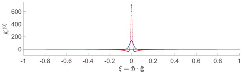
The real part of kernel (G.4) for ε = 0.03 (blue) and ε = 0.01 (red). Points are the result of summing even-order Legendre polynomials in Eq. (G.2) up to l = 1000; solid lines are given by the corresponding analytical formula (G.4). Here, ε controls the peak width, i.e., the vicinity of the equator n̂ · ĝ = 0 in Eq. (G.1) (with ĝ pointing at the North pole), where the fractional derivative (G.6) is evaluated.

Hence, there exists a hierarchy of the kernel coefficients in the SH basis. The coefficients $K_l^{(0)}$ exceed P_l(0) for the FRT, which are in turn greater than the coefficients (A.2) at finite b:

$$\mid K_l(b)\mid \le \mid P_l(0)\mid <\mid K_l^{(0)}\mid \equiv 1<\frac{1}{\mid P_l(0)\mid },$$ (G.7)

since the corresponding functions g_l ≡ K_l(b)/P_l(0) ≤ 1 for all b, at any given l (Jensen et al., 2016). Physically, this reflects that the kernel (G.2) in Eq. (G.1) by design does not magnify or decrease the sharpness of the “reference” ODF ℘⁽⁰⁾(n̂), while the fiber-ball kernel blurs the ODF, and the realistic (finite-b) kernel (2) blurs it even more (that latter kernel is what, presumably, occurs in nature).

Of course, it is the left-hand side of Eq. (G.1), the dMRI signal, that is given, and we are trying to obtain the best approximation for the true ODF ℘(n̂). Deconvolving the ODF from the signal (dividing S_lm by K_l) progressively magnifies the signal’s harmonics with larger l for the FRT in the fiber-ball limit, and even more so for the finite-b case, Fig. 6, in order to compensate for the blurring of the ODF by the diffusion kernel 𝒦. This results in the ODF sharpening (presumably, approaching the realistic ODF, at least in the absence of noise), relative to the minimally-rotated signal ODF ℘⁽⁰⁾ with $p_{lm}^{(0)}=S_{lm}/K_l^{(0)}$. We also note that the original Q-ball ODF reconstruction (Tuch, 2004; Descoteaux et al., 2009) implies p_lm ~ P_l(0)S_lm, i.e. de-emphasizing the signal harmonics with the higher l, which puts Q-ball kernel 1/P_l(0) to the right of | $K_l^{(0)}$| in the hierarchy (G.7).

We can see that our “minimal rotation” of the signal SH coefficients provides a natural reference for the ODF deconvolution methods. We also note an obvious property of the transform (G.1): since ${\left[K_l^{(0)}\right]}^2\equiv 1$, the operator 𝒦̂ ⁽⁰⁾ on a unit sphere applied twice yields identity; equivalently, it equals its inverse.

References

- Alexander DC, Hubbard PL, Hall MG, Moore EA, Ptito M, Parker GJM, Dyrby TB. Orientationally invariant indices of axon diameter and density from diffusion MRI. Neuroimage. 2010;52:1374–1389. doi: 10.1016/j.neuroimage.2010.05.043. [DOI] [PubMed] [Google Scholar]
- Anderson AW. Measurement of fiber orientation distributions using high angular resolution diffusion imaging. Magnetic Resonance in Medicine. 2005;54(5):1194–1206. doi: 10.1002/mrm.20667. [DOI] [PubMed] [Google Scholar]
- Andersson JL, Sotiropoulos SN. An integrated approach to correction for off-resonance effects and subject movement in diffusion MR imaging. NeuroImage. 2016;125:1063–1078. doi: 10.1016/j.neuroimage.2015.10.019. [DOI] [PMC free article] [PubMed] [Google Scholar]
- Assaf Y, Basser PJ. Composite hindered and restricted model of diffusion (CHARMED) MR imaging of the human brain. NeuroImage. 2005;27(1):48–58. doi: 10.1016/j.neuroimage.2005.03.042. [DOI] [PubMed] [Google Scholar]
- Assaf Y, Cohen Y. Non-Mono-Exponential Attenuation of Water and $N$-Acetyl Aspartate Signals Due to Diffusion in Brain Tissue. Journal of Magnetic Resonance. 1998;131:69–85. doi: 10.1006/jmre.1997.1313. [DOI] [PubMed] [Google Scholar]
- Assaf Y, Freidlin RZ, Rohde GK, Basser PJ. New modeling and experimental framework to characterize hindered and restricted water diffusion in brain white matter. Magnetic Resonance In Medicine. 2004 Nov;52(5):965–978. doi: 10.1002/mrm.20274. [DOI] [PubMed] [Google Scholar]
- Barmpoutis A, Jian B, Vemuri BC. Adaptive kernels for multi-fiber reconstruction. Lecture Notes in Computer Science (including subseries Lecture Notes in Artificial Intelligence and Lecture Notes in Bioinformatics) 5636 LNCS. 2009:338–349. doi: 10.1007/978-3-642-02498-6_28. [DOI] [PMC free article] [PubMed] [Google Scholar]
- Basser P, Mattiello J, LeBihan D. Estimation Of The Effective Self-Diffusion Tensor From The {NMR} Spin-Echo. Journal of Magnetic Resonance Series B. 1994;103:247–254. doi: 10.1006/jmrb.1994.1037. [DOI] [PubMed] [Google Scholar]
- Beaulieu C. The basis of anisotropic water diffusion in the nervous system - a technical review. NMR in Biomedicine. 2002;15:435–455. doi: 10.1002/nbm.782. [DOI] [PubMed] [Google Scholar]
- Behrens TEJ, Berg HJ, Jbabdi S, Rushworth MFS, Woolrich MW. Probabilistic diffusion tractography with multiple fibre orientations: What can we gain? NeuroImage. 2007;34(1):144–155. doi: 10.1016/j.neuroimage.2006.09.018. [DOI] [PMC free article] [PubMed] [Google Scholar]
- Bohr A, Mottelson BR. World Scientific. 1998. Nuclear Structure, Vol. II: Nuclear Deformations. [Google Scholar]
- Budde MD, Frank JA. Neurite beading is sufficient to decrease the apparent diffusion coefficient after ischemic stroke. Proc Natl Acad Sci U S A. 2010;107(32):14472–14477. doi: 10.1073/pnas.1004841107. [DOI] [PMC free article] [PubMed] [Google Scholar]
- Callaghan PT, Eccles CD, Xia Y. NMR microscopy of dynamic displacements: k-space and q-space imaging. Journal of Physics E: Scientific Instruments. 1988;21:820–822. [Google Scholar]
- Chklovskii DB, Schikorski T, Stevens CF. Wiring optimization in cortical circuits. Neuron. 2002 Apr;34(3):341–347. doi: 10.1016/s0896-6273(02)00679-7. [DOI] [PubMed] [Google Scholar]
- de Almeida Martins JP, Topgaard D. Two-Dimensional Correlation of Isotropic and Directional Diffusion Using {NMR} Phys Rev Lett. 2016;116:87601. doi: 10.1103/PhysRevLett.116.087601. [DOI] [PubMed] [Google Scholar]
- De Santis S, Jones DK, Roebroeck A. Including diffusion time dependence in the extra-axonal space improves in vivo estimates of axonal diameter and density in human white matter. NeuroImage. 2016;130:91–103. doi: 10.1016/j.neuroimage.2016.01.047. URL http://dx.doi.org/10.1016/j.neuroimage.2016.01.047. [DOI] [PMC free article] [PubMed] [Google Scholar]
- Dell’Acqua F, Rizzo G, Scifo P, Clarke RA, Scotti G, Fazio F. A Model-Based Deconvolution Approach to Solve Fiber Crossing in Diffusion-Weighted MR Imaging. 2007 doi: 10.1109/TBME.2006.888830. [DOI] [PubMed] [Google Scholar]
- Descoteaux M, Deriche R, Knösche TR, Anwander A. Deterministic and probabilistic tractography based on complex fibre orientation distributions. IEEE Transactions on Medical Imaging. 2009;28(2):269–286. doi: 10.1109/TMI.2008.2004424. [DOI] [PubMed] [Google Scholar]
- Dhital B, Kellner E, Kiselev VG, Reisert M. The absence of restricted water pool in brain white matter. NeuroImage. 2017a Nov; doi: 10.1016/j.neuroimage.2017.10.051. URL http://www.sciencedirect.com/science/article/pii/S1053811917308856?via{%}3Dihub. [DOI] [PubMed]
- Dhital B, Kellner E, Reisert M, Kiselev VG. Isotropic diffusion weighting provides insight on diffusion compartments in human brain white matter in vivo. Proceedings of the International Society of Magnetic Resonance in Medicine. 2015;23:2788. [Google Scholar]
- Dhital B, Reisert M, Kellner E, Kiselev VG. Intra-axonal Diffusivity in Brain White Matter. 2017b doi: 10.1016/j.neuroimage.2019.01.015. URL https://arxiv.org/abs/1712.04565. [DOI] [PubMed]
- Dortch RD, Harkins KD, Juttukonda MR, Gore JC, Does MD. Characterizing inter-compartmental water exchange in myelinated tissue using relaxation exchange spectroscopy. Magnetic Resonance in Medicine. 2013;70(5):1450–1459. doi: 10.1002/mrm.24571. [DOI] [PMC free article] [PubMed] [Google Scholar]
- Emsley JW, editor. Nuclear Magnetic Resonance of Liquid Crystals. Springer; Dordrecht: 1985. [Google Scholar]
- Farquharson S, Tournier JD, Calamante F, Fabinyi G, Schneider-Kolsky M, Jackson GD, Connelly A. White matter fiber tractography: why we need to move beyond DTI. Journal of neurosurgery. 2013;118(6):1367–77. doi: 10.3171/2013.2.JNS121294. URL http://thejns.org/doi/full/10.3171/2013.2.JNS121294. [DOI] [PubMed] [Google Scholar]
- Ferizi U, Schneider T, Witzel T, Wald LL, Zhang H, Wheeler-Kingshott CAM, Alexander DC. White matter compartment models for in vivo diffusion MRI at 300mT/m. Neuroimage. 2015 Sep;118:468–483. doi: 10.1016/j.neuroimage.2015.06.027. [DOI] [PubMed] [Google Scholar]
- Fieremans E, Burcaw LM, Lee HH, Lemberskiy G, Veraart J, Novikov DS. In vivo observation and biophysical interpretation of time-dependent diffusion in human white matter. NeuroImage. 2016;129:414–427. doi: 10.1016/j.neuroimage.2016.01.018. [DOI] [PMC free article] [PubMed] [Google Scholar]
- Fieremans E, Jensen JH, Helpern JA. White matter characterization with diffusional kurtosis imaging. Neuroimage. 2011 Sep;58(1):177–188. doi: 10.1016/j.neuroimage.2011.06.006. [DOI] [PMC free article] [PubMed] [Google Scholar]
- Fieremans E, Jensen JH, Helpern JA, Kim S, Grossman RI, Inglese M, Novikov DS. Diffusion Distinguishes Between Axonal Loss and Demyelination in Brain White Matter. Proceedings of the International Society of Magnetic Resonance in Medicine. 2012;20:714. [Google Scholar]
- Fieremans E, Novikov DS, Jensen JH, Helpern JA. Monte {C}arlo study of a two-compartment exchange model of diffusion. NMR in Biomedicine. 2010 Aug;23(7):711–724. doi: 10.1002/nbm.1577. [DOI] [PMC free article] [PubMed] [Google Scholar]
- Ghosh A, Papadopoulo T, Deriche R. Generalized Invariants of a 4th order tensor: Building blocks for new biomarkers in dMRI. CDMRI Workshop, MICCAI; 2012. pp. 165–173. URL http://cmic.cs.ucl.ac.uk/cdmri12/pdfs/p6.pdf. [Google Scholar]
- Girard G, Daducci A, Petit L, Thiran JP, Whittingstall K, Deriche R, Wassermann D, Descoteaux M. AxTract: Toward microstructure informed tractography. Human Brain Mapping. 2017 Nov;38(11):5485–5500. doi: 10.1002/hbm.23741. URL http://doi.wiley.com/10.1002/hbm.23741. [DOI] [PMC free article] [PubMed] [Google Scholar]
- Healy DM, Hendriks H, Kim PTP. Spherical deconvolution. Journal of Multivariate Analysis. 1998;67:1–22. URL http://www.sciencedirect.com/science/article/pii/S0047259X98917572. [Google Scholar]
- Jelescu IO, Veraart J, Fieremans E, Novikov DS. Degeneracy in model parameter estimation for multi-compartmental diffusion in neuronal tissue. NMR in Biomedicine. 2016a;29(1):33–47. doi: 10.1002/nbm.3450. [DOI] [PMC free article] [PubMed] [Google Scholar]
- Jelescu IO, Zurek M, Winters KV, Veraart J, Rajaratnam A, Kim NS, Babb JS, Shepherd TM, Novikov DS, Kim SG, Fieremans E. In vivo quantification of demyelination and recovery using compartment-specific diffusion MRI metrics validated by electron microscopy. Neuroimage. 2016b May;132:104–114. doi: 10.1016/j.neuroimage.2016.02.004. [DOI] [PMC free article] [PubMed] [Google Scholar]
- Jensen JH, Helpern JA, Ramani A, Lu H, Kaczynski K. Diffusional kurtosis imaging: the quantification of non-gaussian water diffusion by means of magnetic resonance imaging. Magn Reson Med. 2005 Jun;53(6):1432–1440. doi: 10.1002/mrm.20508. [DOI] [PubMed] [Google Scholar]
- Jensen JH, Russell Glenn G, Helpern JA. Fiber ball imaging. NeuroImage. 2016 Jan;124:824–833. doi: 10.1016/j.neuroimage.2015.09.049. URL http://www.sciencedirect.com.ezproxy.med.nyu.edu/science/article/pii/S105381191500871X?via{%}3Dihub. [DOI] [PMC free article] [PubMed] [Google Scholar]
- Jespersen SN, Bjarkam CR, Nyengaard JR, Chakravarty MM, Hansen B, Vosegaard T, Ostergaard L, Yablonskiy D, Nielsen NC, Vestergaard-Poulsen P. Neurite density from magnetic resonance diffusion measurements at ultrahigh field: Comparison with light microscopy and electron microscopy. Neuroimage. 2010 Jan;49(1):205–216. doi: 10.1016/j.neuroimage.2009.08.053. [DOI] [PMC free article] [PubMed] [Google Scholar]
- Jespersen SN, Kroenke CD, Ostergaard L, Ackerman JJH, Yablonskiy DA. Modeling dendrite density from magnetic resonance diffusion measurements. Neuroimage. 2007 Feb;34(4):1473–1486. doi: 10.1016/j.neuroimage.2006.10.037. [DOI] [PubMed] [Google Scholar]
- Jespersen SN, Lundell H, Sønderby CK, Dyrby TB. Orientationally invariant metrics of apparent compartment eccentricity from double pulsed field gradient diffusion experiments. NMR in Biomedicine. 2013;26(12):1647–1662. doi: 10.1002/nbm.2999. [DOI] [PubMed] [Google Scholar]
- Jespersen SN, Olesen JL, Hansen B, Shemesh N. Diffusion time dependence of microstructural parameters in fixed spinal cord. 2017 doi: 10.1016/j.neuroimage.2017.08.039. arXiv:1705.03630. [DOI] [PMC free article] [PubMed] [Google Scholar]
- Jian B, Vemuri BC. A Unified Computational Framework for Deconvolution to Reconstruct Multiple Fibers From Diffusion Weighted MRI. 2007 doi: 10.1109/TMI.2007.907552. [DOI] [PMC free article] [PubMed] [Google Scholar]
- Jones DK. Diffusion MRI: Theory, Methods, and Applications. Oxford University Press; New York: 2010. [Google Scholar]
- Kaden E, Kelm ND, Carson RP, Does MD, Alexander DC. Multi-compartment microscopic diffusion imaging. NeuroImage. 2016a;139:346–359. doi: 10.1016/j.neuroimage.2016.06.002. [DOI] [PMC free article] [PubMed] [Google Scholar]
- Kaden E, Knösche TR, Anwander A. Parametric spherical deconvolution: Inferring anatomical connectivity using diffusion MR imaging. NeuroImage. 2007;37(2):474–488. doi: 10.1016/j.neuroimage.2007.05.012. [DOI] [PubMed] [Google Scholar]
- Kaden E, Kruggel F, Alexander DC. Quantitative mapping of the per-axon diffusion coefficients in brain white matter. Magnetic Resonance in Medicine. 2016b;75(4):1752–1763. doi: 10.1002/mrm.25734. [DOI] [PMC free article] [PubMed] [Google Scholar]
- Kazhdan M, Funkhouser T, Rusinkiewicz S. Rotation invariant spherical harmonic representation of 3 d shape descriptors. Symposium on geometry processing. 2003;6:156–164. [Google Scholar]
- Kellner E, Dhital B, Kiselev VG, Reisert M. Gibbs-ringing artifact removal based on local subvoxel-shifts. Magnetic Resonance in Medicine. 2016;76(5):1574–1581. doi: 10.1002/mrm.26054. [DOI] [PubMed] [Google Scholar]
- Khan AR, Chuhutin A, Wiborg O, Kroenke CD, Nyengaard JR, Hansen B, Jespersen SN. Biophysical modeling of high field diffusion MRI demonstrates microstructural aberration in chronic mild stress rat brain. NeuroImage. 2016 doi: 10.1016/j.neuroimage.2016.07.001. [DOI] [PMC free article] [PubMed] [Google Scholar]
- Kiselev VG. The cumulant expansion: an overarching mathematical framework for understanding diffusion {NMR} In: Jones DK, editor. Diffusion {MRI}: Theory, methods and applications. Ch. 10 Oxford University Press; New York: 2010. [Google Scholar]
- Kiselev VG, Il’yasov KA. Is the “biexponential diffusion” biexponential? Magn Reson Med. 2007 Mar;57(3):464–469. doi: 10.1002/mrm.21164. [DOI] [PubMed] [Google Scholar]
- Koay CG, Basser PJ. Analytically exact correction scheme for signal extraction from noisy magnitude {MR} signals. Journal of Magnetic Resonance. 2006;179(2):317–322. doi: 10.1016/j.jmr.2006.01.016. [DOI] [PubMed] [Google Scholar]
- Kroenke CD, Ackerman JJH, Yablonskiy DA. On the nature of the NAA diffusion attenuated MR signal in the central nervous system. Magnetic Resonance in Medicine. 2004;52(5):1052–1059. doi: 10.1002/mrm.20260. [DOI] [PubMed] [Google Scholar]
- Lampinen B, Szczepankiewicz F, M??rtensson J, van Westen D, Sundgren PC, Nilsson M. Neurite density imaging versus imaging of microscopic anisotropy in diffusion MRI: A model comparison using spherical tensor encoding. NeuroImage. 2017;147:517–531. doi: 10.1016/j.neuroimage.2016.11.053. [DOI] [PubMed] [Google Scholar]
- Lasic S, Szczepankiewicz F, Eriksson S, Nilsson M, Topgaard D. Microanisotropy imaging: quantification of microscopic diffusion anisotropy and orientational order parameter by diffusion MRI with magic-angle spinning of the q-vector. Frontiers in Physics. 2014 Feb;2:1–14. URL http://www.frontiersin.org/Biophysics/10.3389/fphy.2014.00011/abstract. [Google Scholar]
- Le Bihan D, editor. Diffusion and Perfusion Magnetic Resonance Imaging. Raven Press; New York: 1995. [Google Scholar]
- Mackay A, Whittall K, Adler J, Li D, Paty D, Graeb D. In vivo visualization of myelin water in brain by magnetic resonance. Magnetic Resonance in Medicine. 1994;31(6):673–677. doi: 10.1002/mrm.1910310614. [DOI] [PubMed] [Google Scholar]
- Mayer JE, Montroll E. Molecular Distribution. The Journal of Chemical Physics. 1941;9(1):2–16. URL http://scitation.aip.org/content/aip/journal/jcp/9/1/10.1063/1.1750822. [Google Scholar]
- McKinnon ET, Jensen JH, Glenn GR, Helpern JA. Dependence on b-value of the direction-averaged diffusion-weighted imaging signal in brain. Magnetic Resonance Imaging. 2016;36:121–127. doi: 10.1016/j.mri.2016.10.026. [DOI] [PMC free article] [PubMed] [Google Scholar]
- Mirzaalian H, Ning L, Savadjiev P, Pasternak O, Bouix S, Michailovich O, Grant G, Marx CE, Morey RA, Flashman LA, George MS, Mcallister TW, Andaluz N, Shutter L, Coimbra R, Zafonte RD, Coleman MJ, Kubicki M, Westin CF, Stein MB, Shenton ME, Rathi Y. NeuroImage Inter-site and inter-scanner diffusion MRI data harmonization. NeuroImage. 2016;135:311–323. doi: 10.1016/j.neuroimage.2016.04.041. URL http://dx.doi.org/10.1016/j.neuroimage.2016.04.041. [DOI] [PMC free article] [PubMed] [Google Scholar]
- Novikov DS, Fieremans E. Relating Extracellular Diffusivity to Cell Size Distribution and Packing Density as Applied to White Matter. Proceedings of the International Society of Magnetic Resonance in Medicine. 2012;20:1829. [Google Scholar]
- Novikov DS, Jensen JH, Helpern JA, Fieremans E. Revealing mesoscopic structural universality with diffusion. Proc Natl Acad Sci U S A. 2014 Apr;111(14):5088–5093. doi: 10.1073/pnas.1316944111. [DOI] [PMC free article] [PubMed] [Google Scholar]
- Novikov DS, Jespersen SN, Kiselev VG, Fieremans E. Quantifying brain microstructure with diffusion MRI: Theory and parameter estimation. 2016 doi: 10.1002/nbm.3998. preprint arXiv:1612.02059. [DOI] [PMC free article] [PubMed] [Google Scholar]
- Reisert M, Kellner E, Dhital B, Hennig J, Kiselev VG. Disentangling micro from mesostructure by diffusion MRI: A Bayesian approach. NeuroImage. 2017;147:964–975. doi: 10.1016/j.neuroimage.2016.09.058. [DOI] [PubMed] [Google Scholar]
- Reisert M, Kiselev VG, Dihtal B, Kellner E, Novikov DS. MesoFT: unifying diffusion modelling and fiber tracking. Medical Image Computing and Computer-Assisted Intervention–MICCAI 2014; Springer; 2014. pp. 201–208. [DOI] [PMC free article] [PubMed] [Google Scholar]
- Ronen I, Budde M, Ercan E, Annese J, Techawiboonwong A, Webb A. Microstructural organization of axons in the human corpus callosum quantified by diffusion-weighted magnetic resonance spectroscopy of N-acetylaspartate and post-mortem histology. Brain Struct Funct. 2014 Sep;219(5):1773–1785. doi: 10.1007/s00429-013-0600-0. [DOI] [PubMed] [Google Scholar]
- Schultz T, Groeschel S. Auto-calibrating spherical deconvolution based on ODF sparsity. Lecture Notes in Computer Science (including subseries Lecture Notes in Artificial Intelligence and Lecture Notes in Bioinformatics) 8149 LNCS (PART 1) 2013:663–670. doi: 10.1007/978-3-642-40811-3_83. [DOI] [PubMed] [Google Scholar]
- Sherbondy AJ, Rowe MC, Alexander DC. MicroTrack: An algorithm for concurrent projectome and microstructure estimation. Lecture Notes in Computer Science (including subseries Lecture Notes in Artificial Intelligence and Lecture Notes in Bioinformatics) 6361 LNCS (PART 1) 2010:183–190. doi: 10.1007/978-3-642-15705-9_23. [DOI] [PubMed] [Google Scholar]
- Skinner NP, Kurpad SN, Schmit BD, Muftuler LT, Budde MD. Rapid In Vivo Detection of Rat Spinal Cord Injury With Double-Diffusion-Encoded Magnetic Resonance Spectroscopy. Magnenetic Resonance in Medicine. 2017;77:1639–1649. doi: 10.1002/mrm.26243. [DOI] [PMC free article] [PubMed] [Google Scholar]
- Sotiropoulos SN, Behrens TEJ, Jbabdi S. Ball and rackets: inferring fiber fanning from diffusion-weighted MRI. NeuroImage. 2012;60(2):1412–1425. doi: 10.1016/j.neuroimage.2012.01.056. [DOI] [PMC free article] [PubMed] [Google Scholar]
- Sotiropoulos SN, Jbabdi S, Xu J, Andersson JL, Moeller S, Auerbach EJ, Glasser MF, Hernandez M, Sapiro G, Jenkinson M, Feinberg DA, Yacoub E, Lenglet C, Van Essen DC, Ugurbil K, Behrens TE. Advances in diffusion MRI acquisition and processing in the Human Connectome Project. NeuroImage. 2013;80:125–143. doi: 10.1016/j.neuroimage.2013.05.057. URL http://dx.doi.org/10.1016/j.neuroimage.2013.05.057. [DOI] [PMC free article] [PubMed] [Google Scholar]
- Stanisz GJ, Szafer A, Wright GA, Henkelman RM. An Analyitical Model of Restricted Diffusion in Bovine Optic Nerve. Magnetic Resonance in Medicine. 1997;37:103–111. doi: 10.1002/mrm.1910370115. [DOI] [PubMed] [Google Scholar]
- Szafer A, Zhong J, Gore JC. Theoretical model for water diffusion in tissues. Magn Reson Med. 1995 May;33(5):697–712. doi: 10.1002/mrm.1910330516. [DOI] [PubMed] [Google Scholar]
- Szczepankiewicz F, Lasivc S, van Westen D, Sundgren PC, Englund E, Westin CF, Strahlberg F, Lätt J, Topgaard D, Nilsson M. Quantification of microscopic diffusion anisotropy disentangles effects of orientation dispersion from microstructure: Applications in healthy volunteers and in brain tumors. NeuroImage. 2015;104:241–252. doi: 10.1016/j.neuroimage.2014.09.057. [DOI] [PMC free article] [PubMed] [Google Scholar]
- Szczepankiewicz F, van Westen D, Englund E, Westin CF, Strahlberg F, Lätt J, Sundgren PC, Nilsson M. The link between diffusion {MRI} and tumor heterogeneity: Mapping cell eccentricity and density by diffusional variance decomposition {(DIVIDE)} NeuroImage. 2016;142:522–532. doi: 10.1016/j.neuroimage.2016.07.038. [DOI] [PMC free article] [PubMed] [Google Scholar]
- Tariq M, Schneider T, Alexander DC, Wheeler-Kingshott CAG, Zhang H. Bingham–NODDI: Mapping anisotropic orientation dispersion of neurites using diffusion MRI. NeuroImage. 2016 doi: 10.1016/j.neuroimage.2016.01.046. [DOI] [PubMed] [Google Scholar]
- Thorne KS. Multipole expansions of gravitational radiation. Reviews of Modern Physics. 1980 Apr;52(2):299–339. [Google Scholar]
- Tournier JD, Calamante F, Connelly A. Robust determination of the fibre orientation distribution in diffusion {MRI}: non-negativity constrained super-resolved spherical deconvolution. Neuroimage. 2007 May;35(4):1459–1472. doi: 10.1016/j.neuroimage.2007.02.016. [DOI] [PubMed] [Google Scholar]
- Tournier JD, Calamante F, Connelly A. Improved probabilistic streamlines tractography by 2nd order integration over fibre orientation distributions. Proc Intl Soc Mag Reson Med. 2010:1670. [Google Scholar]
- Tournier JD, Calamante F, Connelly A. MRtrix: Diffusion tractography in crossing fiber regions. International Journal of Imaging Systems and Technology. 2012;22(1):53–66. [Google Scholar]
- Tournier JD, Calamante F, Connelly A. Determination of the appropriate b value and number of gradient directions for high-angular-resolution diffusion-weighted imaging. NMR in Biomedicine. 2013;26(12):1775–1786. doi: 10.1002/nbm.3017. [DOI] [PubMed] [Google Scholar]
- Tournier JD, Calamante F, Gadian DG, Connelly A. Direct estimation of the fiber orientation density function from diffusion-weighted MRI data using spherical deconvolution. NeuroImage. 2004;23(3):1176–1185. doi: 10.1016/j.neuroimage.2004.07.037. [DOI] [PubMed] [Google Scholar]
- Tournier JDJ, Mori S, Leemans A. Diffusion tensor imaging and beyond. Magnetic Resonance in Medicine. 2011;65(6):1532–56. doi: 10.1002/mrm.22924. URL http://onlinelibrary.wiley.com/doi/10.1002/mrm.22924/full{%}5Cnhttp://scil.dinf.usherbrooke.ca/wp-content/papers/Descoteaux-tsi2012.pdf{%}5Cnhttp://www.pubmedcentral.nih.gov/articlerender.fcgi?artid=3366862{&}tool=pmcentrez{&}rendertype=abstract. [DOI] [PMC free article] [PubMed] [Google Scholar]
- Tuch DS. Q-Ball Imaging. Magnetic Resonance in Medicine. 2004;52:1358–1372. doi: 10.1002/mrm.20279. [DOI] [PubMed] [Google Scholar]
- Unterberg AW, Stover J, Kress B, Kiening KL. Edema and brain trauma. Neuroscience. 2004;129(4):1021–1029. doi: 10.1016/j.neuroscience.2004.06.046. [DOI] [PubMed] [Google Scholar]
- Veraart J, Fieremans E, Novikov DS. Diffusion {MRI} noise mapping using random matrix theory. Magnetic resonance in medicine. 2016a;76:1582–1593. doi: 10.1002/mrm.26059. [DOI] [PMC free article] [PubMed] [Google Scholar]
- Veraart J, Fieremans E, Novikov DS. Universal power-law scaling of water diffusion in human brain defines what we see with {MRI} 2016b preprintarXiv:1609.09145 https://ar.
- Veraart J, Novikov DS, Christiaens D, Ades-Aron B, Sijbers J, Fieremans E. Denoising of diffusion {MRI} using random matrix theory. NeuroImage. 2016c;142:394–406. doi: 10.1016/j.neuroimage.2016.08.016. [DOI] [PMC free article] [PubMed] [Google Scholar]
- Veraart J, Novikov DS, Fieremans E. TE dependent Diffusion Imaging (TEdDI) distinguishes between compartmental T2 relaxation times. NeuroImage. 2017 doi: 10.1016/j.neuroimage.2017.09.030. [DOI] [PMC free article] [PubMed] [Google Scholar]
- Veraart J, Rajan J, Peeters RR, Leemans A, Sunaert S, Sijbers J. Comprehensive framework for accurate diffusion MRI parameter estimation. Magn Reson Med. 2013 Oct;70(4):972–984. doi: 10.1002/mrm.24529. [DOI] [PubMed] [Google Scholar]
- White NS, Dale AM. Optimal diffusion MRI acquisition for fiber orientation density estimation: An analytic approach. Human Brain Mapping. 2009;30(11):3696–3703. doi: 10.1002/hbm.20799. [DOI] [PMC free article] [PubMed] [Google Scholar]
- Wilkins B, Lee N, Gajawelli N, Law M, Lepor?? N. Fiber estimation and tractography in diffusion MRI: Development of simulated brain images and comparison of multi-fiber analysis methods at clinical b-values. NeuroImage. 2015;109:341–356. doi: 10.1016/j.neuroimage.2014.12.060. URL http://dx.doi.org/10.1016/j.neuroimage.2014.12.060. [DOI] [PMC free article] [PubMed] [Google Scholar]
- Yang DM, Huettner JE, Bretthorst GL, Neil JJ, Garbow JR, Ackerman JJ. Intracellular water preexchange lifetime in neurons and astrocytes. Magnetic Resonance in Medicine 00. 2017 Jul; doi: 10.1002/mrm.26781. URL http://doi.wiley.com/10.1002/mrm.26781. [DOI] [PMC free article] [PubMed]
- Zhang H, Schneider T, Wheeler-Kingshott CA, Alexander DC. {NODDI}: practical in vivo neurite orientation dispersion and density imaging of the human brain. Neuroimage. 2012 Jul;61(4):1000–1016. doi: 10.1016/j.neuroimage.2012.03.072. [DOI] [PubMed] [Google Scholar]
Associated Data
This section collects any data citations, data availability statements, or supplementary materials included in this article.